R. Pradhan | K. Swain* | G.C. Dash
OPEN ACCESS
The steady boundary layer viscous incompressible fluid flow on a permeable flat plate embedded in a porous medium has been considered in the present study. The momentum transport phenomena are subjected to external magnetic field, permeability of the porous medium and cross flow due to presence of suction and injection. Moreover, the heat transfer phenomena consider the loss of thermal energy due to radiation and mass transfer phenomena accounts for the generative/destructive chemical reaction of the reactive species as well. Most importantly, the temperature dependent viscosity and thermal conductivity of the fluid makes the present study more realistic. The numerical solution presented through graphs brings out the interesting outcomes: The higher rate of suction enhances the fluid temperature. This observation is akin to the fact that the higher suction brings the molecules closure hence the heat transfer increases. The porous medium, embedding the plate, acts as a coolant by reducing the fluid temperature.
MHD, variable viscosity, variable conductivity, radiation, chemical reaction
The analytical results of Magneto-hydro dynamics (MHD) flow parallel to a flat plate are used to determine the losses at the flat surface such as thin airfoils and side walls of large volume generators and accelerators. Due to number of applications in industrial manufacturing process, the problem of boundary layer flow past a flat plate has attracted the attention of many researchers since a few decades. The flow past a flat plate embedded in a porous medium has drawn the attention of many researchers as the porous material serves as the best coolant and regulates heat transfer. Swain et al. [1] have studied the effects of variable viscosity as well as variable thermal conductivity on stretching sheet embedded in a porous medium. Moalem [2] has studied the steady state heat transfer within porous medium with temperature dependent heat generation. Swain et al. [3] examined the impact of non-uniform heat source/sink on MHD heat and mass transfer on stretching sheet embedded in a porous medium.
The radiative flow of an electrically conducting fluid arises in many real world applications such as in electrical power generation, solar power technology and nuclear reactors. Moreover, radiative heat and mass transfer occur in geo-physical and engineering applications, such as migration of moisture through air contained in fibrous insulations, dispersion and chemical pollutants through water-saturated soil [4, 5]. Radiation effects on boundary layer flow with and without magnetic field have been investigated by Mahmoud [6], Cortell [7], and Bataller [8]. Jat and Chaudhary [9] have presented similarity representation of MHD flow with heat transfer considering variable viscosity and thermal conductivity. Recently, thermal convective surface conditions are prescribed by several authors such as Swain et al. [10], Aziz [11] and Makinde [12] to solve different types of boundary value problems. Hamad et al. [13] considered the radiation effects on heat and mass transfer in MHD stagnation-point flow over a permeable flat plate with thermal convective surface boundary condition, temperature dependent viscosity and thermal conductivity over a permeable porous plate using group transformation and studied the effects of pertinent parameters on flow characteristics. Barik et al. [14] analyzed the effect of chemical reaction and heat source on MHD flow of visco-elastic fluid past an exponentially accelerated vertical plate embedded in a porous medium. Recently, Swain et al. [15] have studied the MHD flow of viscoelastic nanofluid over a stretching sheet. Nayak et al. [16] examined the flow and mass transfer analysis of a micropolar fluid in a vertical channel with heat source and chemical reaction.
To the best of our knowledge not much work has been reported on MHD flow over a permeable flat plate with convective surface boundary conditions as well as variable fluid properties (i) flow through porous medium with uniform porosity (ii) presence of volumetric heat source (iii) reacting species with chemical reaction of first order. In addition to above criteria, the study brings to its fold the works of Alam et al. [17], Bhattacharya [18], and Hamad et al. [13] as particular cases. The results of implicit finite difference method reported in the paper [13] are in good agreement with Runge-Kutta method of solution of the present problem.
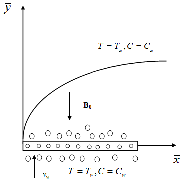
Consider the steady two-dimensional flow of conducting fluid on a surface y=0, the flow being confined to domain y>0. A uniform transverse magnetic field of strength B0 is applied perpendicular to the plate embedded in a fully saturated porous medium. The bottom surface of the permeable plate is heated by a convection current from a hot fluid of temperature Tf. The heat flux applied at the bounding surface gives rise to thermal boundary layer. The fluid properties are supposed to be constant except the dynamic viscosity and thermal conductivity. The flow is also affected by the cross flow i.e. suction/injection at the plate. The ambient state (free stream) velocity, temperature and concentration are denoted as ${{\bar{u}}_{\infty }}(\bar{x})\,,\,\,{{T}_{\infty }}\,\,\text{and}\,\,{{C}_{\infty }}.$ Figure 1 shows the flow geometry.
Figure 1. Flow geometry
The flow model assumes that no particle coagulation occurs and the magnetic Reynolds number as well as the electric field owing to polarization of charges is negligible. The governing equations following Kays et al. [19] and Hamad et al. [13] are given by:
$\frac{\partial \bar{u}}{\partial \bar{x}}+\frac{\partial \bar{v}}{\partial \bar{y}}\,=\,0$ (1)
$\rho \left( \bar{u}\,\frac{\partial \bar{u}}{\partial \bar{x}}+\,\,\text{\bar{v}}\frac{\partial \bar{v}}{\partial \bar{y}} \right)\,=-\,\,\frac{\partial p}{\partial \,\bar{x}}+\mu \frac{{{\partial }^{2}}\bar{u}\,}{\partial {{{\bar{y}}}^{2}}}+\,\frac{\partial \mu }{\partial T}\,\,\frac{\partial T}{\partial \bar{y}}\,\frac{\partial \,\bar{u}}{\partial \,\bar{y}}\,-\,\sigma B_{0}^{2}\bar{u}\,\,-\,\frac{\mu \bar{u}}{k_{p}^{*}}$ (2)
$\rho {{c}_{p}}\left( \bar{u}\,\,\frac{\partial T}{\partial \,\bar{x}}\,+\,\,\text{\bar{v}}\frac{\partial \,T}{\partial \,\bar{y}}\, \right)\,=\,\,\,\frac{\partial }{\partial \,\bar{y}}\,\,\left( K(T)\,\frac{\partial T}{\partial \,\bar{y}}\,\, \right)-\,\,\,\frac{\partial {{q}_{r}}}{\partial \,\bar{y}}+Q(T-{{T}_{\infty }})$ (3)
$\bar{u}\,\,\frac{\partial C}{\partial \,\bar{x}}\,+\,\,\text{\bar{v}}\frac{\partial C}{\partial \,\bar{y}}\,\,=\,\,{{D}_{m}}\,\frac{{{\partial }^{2}}C}{\partial \,{{{\bar{y}}}^{2}}}\,-\,\gamma C$ (4)
The boundary conditions are:
$\left. \begin{align} & \bar{u}\,=\,0\,,\,\,\text{\bar{v}}\,=\,-{{\text{v}}_{w}}\,,\,\,-K\frac{\partial T}{\partial \bar{y}}\,=\,{{h}_{f}}\,[{{T}_{f}}-{{T}_{w}}]\,,\,C=\,{{C}_{w}}\,\text{at}\,\,\bar{y}=0 \\ & \bar{u}\to \,{{{\bar{u}}}_{\infty }}\,(\bar{x})\,,\,\,T\to {{T}_{\infty }}\,,\,\,C\to {{C}_{\infty }}\,\,\text{at}\,\,\bar{y}\to \infty \\ \end{align} \right\}$ (5)
where, subscripts $w, \infty$ denote wall conditions and free stream conditions respectively.
The pressure distribution in the boundary layer is a function of x only, i.e. for a given x, P is constant throughout the boundary layer and can be evaluated using Euler equation of potential flow (just outside the boundary layer) by Yuan [20].
In the free stream $\bar{u}\,=\,{{\bar{u}}_{\infty }}\,(\bar{x})$. and hence Eq. (2) reduces to:
${{\bar{u}}_{\infty }}\,\frac{d\,{{{\bar{u}}}_{\infty }}}{d\,\bar{x}}=-\frac{1}{\rho }\,\,\frac{\partial p}{\partial \bar{x}}-\frac{\sigma B_{0}^{2}}{\rho }\,\,{{\bar{u}}_{\infty }}\,(\bar{x})-\,\frac{\nu {{{\bar{u}}}_{\infty }}(\bar{x})}{k_{p}^{*}}$ (6)
Eliminating the pressure gradient term $(\partial p/\partial \,\bar{x})$ between Eqns. (2) and (6), we get:
${{\bar{u}}_{\infty }}\,\frac{\partial \,{{{\bar{u}}}_{\infty }}}{\partial \,\bar{x}}+\bar{v}\frac{\partial \,\bar{u}}{\partial \,\bar{y}}\,=\,{{\bar{u}}_{\infty }}\,\frac{d\,{{{\bar{u}}}_{\infty }}}{d\,\bar{x}}\,+\,\nu \,\frac{{{\partial }^{2}}\bar{u}}{\partial \,{{{\bar{y}}}^{2}}}-\,\frac{\sigma B_{0}^{2}}{\rho }\,(\bar{u}\,-\,{{\bar{u}}_{\infty }})-\frac{\nu }{k_{p}^{*}}(\bar{u}\,-\,{{\bar{u}}_{\infty }})$ (7)
The temperature dependent viscosity and thermal conductivity vary linearly (Seddeek and Salem [21]) as:
$\mu (T)\,=\,{{\mu }_{\infty }}\,[{{a}_{0}}+{{b}_{0}}\,({{T}_{f}}-T)]\,\,,\,\,K(T)\,=\,{{k}_{\infty }}[1+c(T-{{T}_{\infty }})]$ (8)
where, ${{\mu }_{\infty }}\,,\,{{k}_{\infty }}$ are the constant undisturbed viscosity and undisturbed thermal conductivity, a0, b0 are a constant with b0>0, c is a constant which depends on the fluid. For our calculation the choice of a0=1.
The radiative heat flux ${{q}_{r}}$ along $\bar{y}$ direction is described by the Rosseland approximation as ${{q}_{r}}\,=\,-\frac{4{{\sigma }_{1}}}{3{{k}_{1}}}\,\frac{\partial {{T}^{4}}}{\partial \,\bar{y}},{{T}^{4}}\,\cong \,\,4TT_{\infty }^{3}-\,3T_{\infty }^{4}$ we get:
$\frac{\partial {{q}_{r}}}{\partial \,\bar{y}}\,=-\,\frac{16{{\sigma }_{1}}T_{\infty }^{3}}{3{{k}_{1}}}\,\frac{{{\partial }^{2}}T}{\partial \,{{{\bar{y}}}^{2}}}$ (9)
where, σ1 is the Stefan-Boltzman constant and k1 is the mean absorption coefficient.
Using (8) and (9), the Eq. (3) becomes,
$\bar{u}\,\frac{\partial T}{\partial \bar{x}}+\bar{v}\,\frac{\partial T}{\partial \bar{y}}\,=\frac{{{k}_{\infty }}}{\rho {{c}_{p}}}\,\frac{\partial }{\partial \bar{y}}\,\left( (1+K\theta )\,\,\frac{\partial T}{\partial \bar{y}} \right)+\,\frac{16{{\sigma }_{1}}T_{\infty }^{3}}{3\rho {{c}_{p}}{{k}_{1}}}\,\,\frac{{{\partial }^{2}}T}{\partial \,{{{\bar{y}}}^{2}}}+\frac{Q}{\rho {{c}_{p}}}(T-{{T}_{\infty }})$ (10)
The quantity $K=c({{T}_{f}}-{{T}_{\infty }})$ is termed as thermal conductivity parameter.
Introducing the following dimensionless variables and parameters.
$\begin{align} & x=\,\frac{{\bar{x}}}{L}\,\,,\,\,y=\,\frac{\bar{y}\,\sqrt{R\,e}}{L}\,\,,\,\,u\,\,=\,\frac{{\bar{u}}}{{{U}_{\infty }}}\,,\,v\,=\,\frac{\bar{v}\sqrt{Re}}{{{U}_{\infty }}},\,{{u}_{\infty }}=\,\frac{{{{\bar{u}}}_{\infty }}}{{{U}_{\infty }}}, \\ & \theta \,=\,\frac{T-{{T}_{\infty }}}{{{T}_{f}}-{{T}_{\infty }}}\,,\,\phi \,=\,\,\frac{C-{{C}_{\infty }}}{{{C}_{w}}-{{C}_{\infty }}},M=\,\,\frac{\sigma B_{0}^{2}L}{\rho {{U}_{\infty }}}, \\ \end{align}$
$\begin{align} & {{k}_{p}}=\,\frac{\nu L}{k_{p}^{*}{{U}_{\infty }}}\,,Sc\,=\,\frac{\nu }{{{D}_{m}}}\,,\,Pr\,=\,\frac{{{\mu }_{\infty }}{{c}_{p}}}{{{k}_{\infty }}},\,A\,\,=\,\,b({{T}_{f}}-{{T}_{\infty }})\,,\, \\ & R\,=\,\frac{4{{\sigma }_{1}}T_{\infty }^{3}}{{{k}_{1}}{{k}_{\infty }}},\,S=\frac{Q(T-{{T}_{\infty }})}{\rho {{c}_{p}}}\,,\,{{k}_{c}}=\,\frac{{{U}_{\infty }}{{L}^{2}}}{{{R}_{e}}} \\ \end{align}$
Introducing the stream function ψ, defined by:
$u\,=\,\frac{\partial \psi }{\partial \,y}\,\,\,,\,\,\,v\,=\,-\frac{\partial \psi }{\partial x}$
We get the following transformed momentum, energy, and concentration equations,
$\frac{\partial \psi }{\partial y}\,\frac{{{\partial }^{2}}\psi }{\partial x\partial y}\,-\,\frac{\partial \psi }{\partial x}\,\frac{{{\partial }^{2}}\psi }{\partial {{y}^{2}}}\,-{{u}_{\infty }}\,\frac{d{{u}_{\infty }}}{dx}\,-\left[ \,1+A\,(1-\theta ) \right]\,\frac{{{\partial }^{3}}\psi }{\partial {{y}^{3}}}$$+\,A\frac{{{\partial }^{2}}\psi }{\partial {{y}^{2}}}\,\frac{\partial \theta }{\partial y}+(M+{{k}_{p}})\,\left( \frac{\partial \psi }{\partial y}-{{u}_{\infty }} \right)\,\,=\,\,0\,,$ (11)
$\begin{align} & \,\frac{\partial \psi }{\partial y}\,\frac{\partial \theta }{\partial x}\,-\,\frac{\partial \psi }{\partial x}\,\frac{\partial \theta }{\partial y}\,-\,\frac{1}{Pr}\,\left[ 1+K\theta \,+\frac{4R}{3} \right]\,\, \\ & \frac{{{\partial }^{2}}\theta }{\partial {{y}^{2}}}-\frac{1}{Pr}K\,{{\left( \frac{\partial \theta }{\partial y} \right)}^{2}}+S\theta =0 \\ \end{align}$ (12)
$\,\frac{\partial \psi }{\partial y}\,\frac{\partial \phi }{\partial x}\,-\,\frac{\partial \psi }{\partial x}\,\frac{\partial \phi }{\partial y}\,-\,\frac{1}{Sc}\,\frac{{{\partial }^{2}}\phi }{\partial {{y}^{2}}}\,+{{k}_{c}}\phi =\,0$ (13)
The corresponding boundary conditions (5) are given by:
$\begin{align} & \frac{\partial \psi }{\partial y}\,=\,0\,,\,\,\frac{\partial \psi }{\partial x}\,=\,-\frac{{{v}_{m}}}{{{U}_{\infty }}\sqrt{Re}}\,\,,\frac{\partial \theta }{\partial y}=-\frac{L{{h}_{f}}}{\sqrt{Re}}\,\left[ \frac{1-\theta (0)}{1+K\theta (0)} \right]\,, \\ & \phi =1\,\,\,\,\,\,\,\text{at}\,\,\,\,y=\,0\, \\ & \frac{\partial \psi }{\partial y}\,\to \,x\,,\,\,\theta \to 0,\,\,\phi \to 0\,\,\,\,\text{as}\,y\to \infty \\ \end{align}$ (14)
Using the similarity transformation η=xf(y) in Eqns. (11)-(14), we get:
$\begin{align} & (1+A\,(1-\theta ))\,\,{f}'''+(f-A{\theta }')\,{f}''\,-\,(M+{{k}_{p}}) \\ & ({f}'-1)-{{{{f}'}}^{2}}+1=0 \\ \end{align}$ (15)
$\left[ 1+K\theta +\frac{4R}{3} \right]\,\,{\theta }''+K{{{\theta }'}^{2}}+\Pr f{\theta }'+S\theta =\,\,0\,$ (16)
${\phi }''+Sc\,f{\phi }'-Sc{{k}_{c}}\,\phi =\,0.$ (17)
$\begin{align} & f(0)\,=\,{{f}_{w}}\,,\,\,{f}'\left( 0 \right)=0\,\,,\,\,\theta (0)\,=\,\frac{1+b{\theta }'(0)}{1-Kb{\theta }'(0)}\,,\, \\ & \,\phi \left( 0 \right)=1\,\,\,\,\,\text{at}\,\,\,\eta =0 \\ & {f}'\left( \eta \right)\to 1\,,\,\,\theta \left( \eta \right)\to 0\,,\,\,\phi \left( \eta \right)\to 0\,\,as\,\,\,\eta \to \infty \\ \end{align}$ (18)
The expressions for skin friction, rate of heat transfer and rate of mass transfer at the surface $\bar{y}=0$ are given by:
$\begin{align} & {{C}_{f}}=\frac{\mu }{\rho \bar{u}_{\infty }^{2}}{{\left( \frac{\partial \bar{u}}{\partial \bar{y}} \right)}_{\bar{y}=0}}\,\,,\,\,\,Nu=\,\frac{-\bar{x}}{{{T}_{f}}-{{T}_{\infty }}}{{\left( \frac{\partial T}{\partial \bar{y}} \right)}_{\bar{y}=0}}\,,\,\, \\ & Sh=\,\frac{-\bar{x}}{{{C}_{w}}-{{C}_{\infty }}}{{\left( \frac{\partial C}{\partial \bar{y}} \right)}_{\bar{y}=0}}\, \\ \end{align}$ (19)
And their corresponding non-dimensional forms are:
$\begin{align} & R{{e}^{\tfrac{1}{2}}}{{C}_{f}}=\left[ 1+A\,(1-\theta \,(0) \right]\,{f}''(0), \\ & R{{e}^{-\tfrac{1}{2}}}Nu\,=-{\theta }'(0)\,,R{{e}^{-\tfrac{1}{2}}}Sh\,=-\,{\phi }'(0)\, \\ \end{align}$ (20)
Numerical integration by Runge-Kutta method for solving Eqns. (15)-(17), exactly we shall adopt a step-by-step integration method along with shooting technique, by converting the two-point boundary value problem (BVP) into an initial value problem (IVP). In this method, the equations are reduced to a set of first order differential equations:
$\begin{align} & {f}'=p \\ & {p}'=q \\ & {\theta }'=r \\ & {\phi }'=s \\ & {q}'=\frac{1}{1+A\left( 1-\theta \right)}\left[ \left( Ar-f \right)q+\left( M+{{k}_{p}} \right)\left( p-1 \right)+{{p}^{2}}-1 \right] \\ \end{align}$ (21)
${r}'=\frac{-3}{3\left( 1+K\theta \right)+4R}\left[ K{{r}^{2}}+\Pr fr+S\theta \right]$ (22)
${s}'=-Sc\left[ fs-{{k}_{c}}\phi \right]$ (23)
with the initial conditions:
$\begin{align} & f\left( 0 \right)={{f}_{w}} \\ & p\left( 0 \right)=0 \\ & \theta \left( 0 \right)=\frac{1+br\left( 0 \right)}{1-Kbr\left( 0 \right)} \\ \end{align}$ (24)
To start the integration it is necessary to know all the required values at η=0 from which we start our forward integration. In the present problem q(0), r(0) and s(0) are not known. So, we are to provide the guess values to the unknowns along with known values to start the integration. There is an inbuilt self-corrective procedure in the MATLAB coding to correct the unknown guess values. Ones the corrected values are attended then the step-by-step integration by Runge-Kutta method is performed and the solution is obtained within the prescribed error limit by Howard [22].
The system of Eqns. (15)-(17) with boundary conditions Eq. (18) are solved numerically by Runge-Kutta method with shooting technique. Figures 2 and 3 show that the results are in good agreement with the earlier work [13]. In the computation, we have restricted to low value of Sc which is consistent for air medium. The diffusing species are common gasses such as hydrogen (Sc=0.22), ammonia (Sc=0.78), Sc=0.1 (arbitrary). Further, we have restricted our discussion to a constant convective parameter b= 0.1.
Figure 2 has been carefully designed to display momentum, thermal and solutal transport phenomena in the form of velocity, temperature, and concentration profiles. This validates our observation in the absence of additional parameters appeared in the governing equations. The effect of suction parameter fwis to increase the velocity irrespective of the presence or absence of porous medium but the reverse effect is observed in case of temperature and concentration distribution. The same observation was reported by Hamad et al. [13] as outlined below. It can be observed that the velocity ${f}'$ rises whilst temperature and concentration fall with rising fw. Also, we have noticed that the thickness of momentum, thermal and concentration boundary layers reduce with rising fw. Due to higher suction the fluid particles are brought closure. Hence, the thickness of the boundary layer decreases. Thus, vorticity diffusion is prevented. The physical interpretation of the figure also remains same but the numerical values of velocity, temperature and concentration at a fixed point say at η=0.2 appears slightly higher in our case which can be attributed to the presence of porous medium kp=0.5. Another interesting conclusion we derive in case of thinning of three boundary layers with an increasing suction which agrees well with the earlier work reported in literature.
Figure 3 exhibits the effect of suction on temperature distribution. The curve I for kp=0, S=0 and kc=0 represents the work [13]. It is observed that temperature increases with higher value of heat source parameter. This is obvious due to increase in heat source parameter leads to higher diffusion of heat energy, so that temperature rises. Further, it is seen that presence of porous matrix reduces the temperature and acts as a coolant where as suction increases the temperature.
Figure 2. Effect of fw on velocity, temperature and concentration distributions for S=0, Pr=0.7, M=0.1, R=1, Sc=0.1, A=0.1, K=0.5, a=1 and b=0.1
Figure 3. Effect of fw, S and kp on temperature distribution for Pr=0.7, M=0.1, R=1, Sc=0.1, A=0.1, K=0.5, a=1 and b=0.1
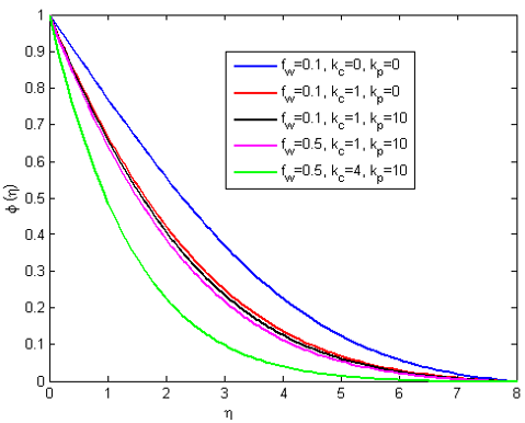
Figure 4 exhibits the concentration variation in response to rate of chemical reaction parameter kc. It is observed that an increase in kc from 0.0 to 4.0, leads to decrease the level of concentration because the increasing rate of destructive reaction (kc>0) the level of concentration is depleted.
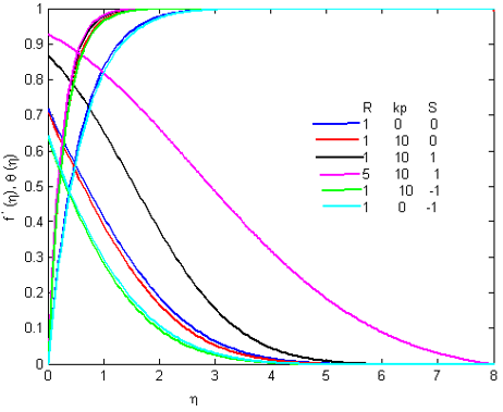
Figure 5 shows the effect of radiation on velocity and temperature. It is observed that increase in radiation contribute to enhance the velocity as well as temperature distribution in the entire flow domain because the radiative heat energy increases the momentum transport as well as thermal diffusion. The same observation was also made by Hamad et al. [13].
Figure 4. Effect of fw, kc and kp on concentration distribution for Pr=0.7, M=0.1, R=1, Sc=0.1, A=0.1, K=0.5, a=1 and b=0.1
Figure 5. Effect of R, kp and S on velocity and temperature distributions for Pr=0.7, M=0.1, R=1, Sc=0.1, A=0.1, K=0.5, a=1 and b=0.1
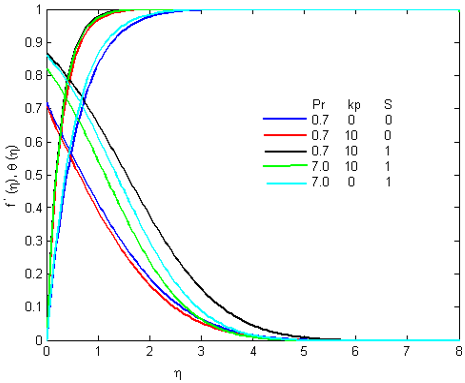
Figure 6 displays the effects of Pr on velocity and temperature distribution. Prandtl number signifies the ratio of momentum diffusivity to thermal diffusivity. Fluid with lower Pr will possess higher conductivity. The role of Prandtl number is quite important in predicting the flow characteristics because this represents the ratio of kinematic viscosity and thermal diffusivity. Therefore, it is a measure of relative importance of viscosity and thermal diffusivity. Profiles for Pr=0.7 and 7 are relates to air and water respectively. It is clear from Figure 6 that an increase in S and kp, enhances both velocity and temperature whereas opposite effect is observed in case of Pr.
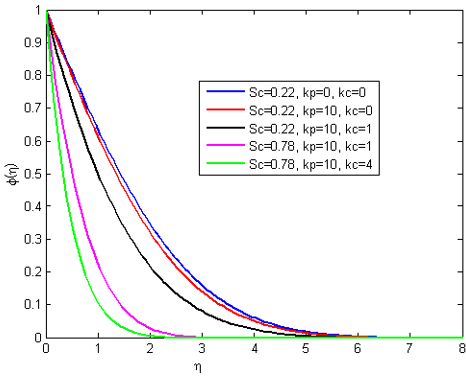
Figure 7 shows the effects of Schmidt number (Sc) and chemical reaction parameter (kc) on concentration profile. The Sc measures the molecular diffusivity of the chemical species. The values of Sc correspond to diffusing species of common interest in air medium. Sc=0.24, 0.30, 0.78 and 1.02 correspond to He, H2, NH3 and CO2. The higher the Sc, heavier the species and lower the diffusivity property. It is observed that heavier species decrease the concentration. A higher value of Sc implies lower diffusion which causes fall of concentration. Similarly, the case of higher rate of chemical reaction explained earlier.
Figure 6. Effect of Pr, kp and S on velocity and temperature distributions for M=0.1, R=1, Sc=0.1, A=0.1, K=0.5, a=1 and b=0.1
Figure 7. Effect of Sc, kp and kc on concentration distribution for Pr=0.7, M=0.1, R=1, A=0.1, K=0.5, a=1 and b=0.1
From the present study the following conclusions are drawn:
1. Higher values of volumetric heat source and suction enhance the temperature distribution since the higher suction brings the molecules closure, hence heat transfer increases but the presence of porous matrix reduces it. Therefore, embedding the plate in a porous medium acts as an insulation not allowing heat to pass from the plate to the fluid.
2. Higher rate of destructive chemical reaction causes a fall in concentration. The above discussion is restricted to a constant value of convective parameter b, which appears in the boundary condition $\theta (0)=\frac{1+b{\theta }'(0)}{1-Kb{\theta }'(0)}$. This condition pertaining to a surface temperature is responsible for convective heat. If b=0, implies θ(0)=1, a case of constant temperature at the plate. We have assigned b=0.1, K=0.5 in our study so that the result relates to constant thermal convection and conduction. For constant heat conduction, for fixed K, higher rate of convection leads to rise in plate temperature, so that temperature of the fluid falls which leads to decrease in momentum transport, resulting decrease in velocity (reported by Hamad et al. [13]).
|
$\bar{u},\bar{v}$ |
velocity components along $\bar{x}$ and $\bar{y}$ axis |
|
T, C |
fluid temperature, species concentration |
|
Tw, Cw |
wall temperature, wall species concentration |
|
T∞, C∞ |
temperature and concentration in the free stream |
|
vw |
mass transfer velocity |
|
ν=μ/ρ |
kinematic coefficient of viscosity |
|
μ, ρ |
coefficient of viscosity, density of the fluid |
|
σ, k |
electric conductivity, thermal conductivity |
|
α, cp |
thermal diffusivity, specific heat at constant pressure |
|
Dm = k/ρcp |
mass diffusivity of species in fluid |
|
hf, B0 |
heat transfer coefficient, magnetic field strength |
|
qr, σ1, k1 |
radiative heat flux, Stefan-Boltzman constant, mean absorption coefficient |
|
S, M |
heat source/sink parameter, magnetic parameter |
|
A, R |
viscosity parameter, radiation parameter |
|
b, fw |
convective heat transfer parameter, suction/injection parameter |
|
kp, kc |
porosity parameter, chemical reaction parameter |
[1] Swain, K., Parida, S.K., Dash, G.C. (2017). MHD heat and mass transfer on stretching sheet with variable fluid properties in porous medium. Modelling, Measurement and Control B, 86(3): 706-726. https://doi.org/10.18280/mmc_b.860307
[2] Moalem, D. (1976). Steady state heat transfer within porous medium with temperature dependent heat generation. International Journal Heat and Mass Transfer, 19(5): 529-537. https://doi.org/10.1016/0017-9310(76)90166-6
[3] Swain, K., Parida, S.K., Dash, G.C. (2018). Effects of non-uniform heat source/sink and viscous dissipation on MHD boundary layer flow of Williamson nanofluid through porous medium. Defect and Diffusion Forum, 389: 110-127. https://doi.org/10.4028/www.scientific.net/DDF.389.110
[4] Mahmoud, M.A.A. (2009). Thermal radiation effect on unsteady MHD free convection flow past a vertical plate with temperature-dependent viscosity. The Canadian Journal of Chemical Engineering, 87(1): 47-52. https://doi.org/10.1002/cjce.20135
[5] Chamkha, A.J. (2001). Coupled heat and mass transfer by natural convection about a truncated cone in the presence of magnetic field and radiation effects. Numerical Heat Transfer, Part A: Applications, 39(5): 511-530. https://doi.org/10.1080/10407780120202
[6] Mahmoud, M.A.A. (2007). Variable viscosity effects on hydromagnetic boundary layer flow along a continuously moving vertical plate in the presence of radiation. Applied Mathematical Sciences, 1(17): 799-814.
[7] Cortell, R. (2008). Effects of viscous dissipation and radiation on thermal boundary layer over a nonlinearly stretching sheet. Physics Letters A, 372(5): 631-636. https://doi.org/10.1016/j.physleta.2007.08.005
[8] Bataller, R.C. (2008). Radiation effects on Blasius flow. Applied Mathematics and Computation, 198(1): 333-338. https://doi.org/10.1016/j.amc.2007.08.037
[9] Jat, R.N., Chaudhary, S. (2010). Radiation effects on the MHD flow near the stagnation point of a stretching sheet. Zeitschrift Für Angewandte Mathematik Und Physik, 61(6): 1151-1154. https://doi.org/10.1007/s00033-010-0072-5
[10] Swain, K., Parida, S.K., Dash, G.C. (2018). Thermal slip effect on MHD convective nanofluid flow over a vertical plate embedded in a porous medium. European Journal of Electrical Engineering, 20(2): 215-233. https://doi.org/10.3166/ejee.20.215-233
[11] Aziz, A. (2009). A similarity solution for laminar thermal boundary layer over flat plate with convective surface boundary condition. Communications in Nonlinear Science and Numerical Simulation, 14(4): 1064-1068. https://doi.org/10.1016/j.cnsns.2008.05.003
[12] Makinde, O.D. (2010). On MHD heat and mass transfer over a moving vertical plate with a convective surface boundary condition. The Canadian Journal of Chemical Engineering, 88(6): 983-990. https://doi.org/10.1002/cjce.20369
[13] Hamad, M.A.A., Uddin, M.J., Ismail, A.I.M. (2012). Radiation effects on heat and mass transfer in MHD stagnation point flow over a permeable flat plate with thermal convective surface boundary condition, temperature dependent viscosity and thermal conductivity. Nuclear Engineering and Design, 242: 194-200. https://doi.org/10.1016/j.nucengdes.2011.09.005
[14] Barik, R.N., Dash, G.C., Rath, P.K. (2015). Chemical reaction and heat source effects on MHD flow of visco-elastic fluid past an exponentially accelerated vertical plate embedded in a porous medium. Modelling, Measurement and Control B, 84(2): 80-104.
[15] Swain, K., Parida, S.K., Dash, G.C. (2018). MHD flow of viscoelastic nanofluid over a stretching sheet in a porous medium with heat source and chemical reaction. Annales de Chimie - Science des Matériaux, 42(1): 7-21. https://doi.org/10.3166/ACSM.42.7-21
[16] Nayak, M.K., Dash, G.C., Singh, L.P. (2015). Flow and mass transfer analysis of a micropolar fluid in a vertical channel with heat source and chemical reaction. Modelling, Measurement and Control B, 84(1): 69-91.
[17] Alam, M.S., Rahman, M.M., Sattar, M.A. (2008). Effects of variable suction and thermophoresis on steady MHD combined free-forced convective heat and mass transfer flow over a semi-infinite permeable inclined plate in the presence of thermal radiation. International Journal of Thermal Sciences, 47(6): 758-765. https://doi.org/10.1016/j.ijthermalsci.2007.06.006
[18] Bhattacharyya, K., Mukhopadhyay, S., Layek, G.C. (2011). Slip effects on boundary layer stagnation-point flow and heat transfer towards a shrinking sheet. International Journal of Heat and Mass Transfer,54(1-3): 308-313. https://doi.org/10.1016/j.ijheatmasstransfer.2010.09.041
[19] Kays, W.M., Crawford, M.E., Weigand, B. (2004). Convective Heat and Mass Transfer, 4th Edition. Mcgraw-Hill Series in Mechanical Engineering, New York.
[20] Yuan, S.W. (1969). Foundations of Fluid Dynamics. Prentice Hall of India, p. 308.
[21] Seddeek, M.A., Salem, A.M. (2005). Laminar mixed convection adjacent to vertical continuously stretching sheets with variable viscosity and variable thermal diffusivity. Heat and Mass Transfer, 41: 1048-1055. https://doi.org/10.1007/s00231-005-0629-6
[22] Howard, P. (2007). Solving ODE in MATLAB. https://www.math.tamu.edu/undergraduate/research/REU/comp/matode.pdf, accessed on October 17, 2019.