Kaustubh G. Kulkarni* | Sanjay N. Havaldar | Pradip K. Tamkhade | Amit D. Desale | Sandeep P. Nalavade
© 2024 The authors. This article is published by IIETA and is licensed under the CC BY 4.0 license (http://creativecommons.org/licenses/by/4.0/).
OPEN ACCESS
The central tower solar receiver system is comprised of a number of small tracing mirrors that focus the beam radiation onto a huge tower in the centre. The tracing mirrors are placed as well as adjusted in such a manner that the light is always reflected at the top of the tower. The major goal of this study is to carry out a mathematical assessment of the central tower solar receiver where solar load calculation and heat transfer analysis has been carried out. Solar load is calculated for the location of Pune, India. Mathematical modelling is performed for the solar central receiver system Results of the mathematical modelling reveal that the estimated average sunshine hour for the year ranges from 10.9 hours in the month of December to 12.9 hours in the month of July. The maximum incident beam radiation of 1050.9 w/m2 has been estimated in the month of April at 1200 hour. After computing the variables, the matrix equation can be generated and the system can calculate the energy under the first-order differential equation. The system’s thermal efficiency can be computed once the maximum temperature of the heat transfer fluid, ambient air as well as copper tube is known.
mathematical modeling, solar receiver, heliostats, solar irradiances, energy balance, central solar tower
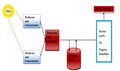
Solar thermal technologies work by concentrating solar energy to make steam, which may then be utilized for generating electricity with the use of standard thermodynamic power cycles. CSP-based systems focus the sun's direct solar energy on a receiver, it is made to effectively absorb all radiation that comes into contact with it. The thermodynamic power cycle operating fluid then receives the heat that was first absorbed, and this fluid drives the power block to produce electricity. It is preferable for the receiver to absorb as much incident radiation as possible for increasing the Heat Transfer Fluid temperature. This may increase the working fluid's temperature when it is pumped into the turbines, increasing their capacity to produce work. Because of the high concentration ratio, point-focus-based technologies obtain greater temperatures at the receiver (700–1000℃), whereas technologies based on line-focus achieve lower temperatures as heat losses in HTF transit [J P Bijarniya 2016].
1.1 Working principle of central tower solar receiver
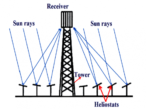
One kind of concentrated collector system is named as a power tower. The beam emission in this system is focused onto a large tower in the middle by a collection of tiny tracing mirrors. The positioning and adjusting of the tracing mirrors ensure that the sunlight is continually mirrored at the tower's highest point. The tower receives a concentrated solar flux that ranges in value from 200 to 1000 kw/m2, allowing for operation at temperatures as high as 1500℃ on average. In Figure 2, a power tower is seen.
Figure 1. Concept of CSP technologies
Figure 2. Working principle of central tower solar receiver
Adoption of renewable energy technologies for India's sustainable development is a critical approach in scientific research in the energy generation field, particularly technologies that generate such types of energy. According to literature surveys, a significant amount of scientific research has been conducted by Laporte (2021) in order to expand the system's functionality that generates energy from these resources. Manzoo's work on time resolution assessment was used to estimate the central solar receiver (2021).
A theoretical study of convection in volumetrically absorbing solar thermal receivers, Mishra (2020). Evaluation of three methods to establish the slant path meteorological intensification of the center receiver, Madjid (2020). Satyavan's work on the novel hybridization of the solar central receiver system (2020). A quantitative analysis of the spiral solar receiver's thermal evaluation for such a centralized transmitter system is required, Chen (2019).
An investigation into the high temperature features of chemical vapor-deposited AlN coatings for solar central receivers, Fang (2019). An air curtain-equipped solar central cavity receiver's natural convective heat loss is being investigated numerically, Ayad (2018). Create a New Detector for the Solar Energy's Prime Tower, Danyela (2018). Based on observed data of direct direct sunlight, ocular risks are assessed in a central transmitter solar power facility, Andreas (2017). Utilizing molten salt and liquid metals, solar central reception tubes’ transient CFD and FEM computations are compared, Danyela (2017). Examining the cumulative and instantaneous skin radiation exposures in central receivers solar systems, Danyela (2016). An analysis of solar levels of exposure at work in concentrating solar power systems, Reyes (2016). A pressurized carbon dioxide cycle's optimization for a cutting-edge central receiver, Alberto (2015).
A projection approach for an analytical function to determine how solar radiation will affect central receivers, J. Coventry (2015). An analysis of central receiver potassium receiver technologies, Bruno (2014). Optimization of a primary radio transmitter for environmental air volume, Maria (2014). Study and comparison of CFD simulations for molten salt external receiver and streamlined thermal performance models, Pacio (2013). An assessment of liquid metal technologies is needed, as well as future directions for using them as effective heat transfer medium in solar central receiver systems, Huang (2013). Forecasting and improving the effectiveness of the parabolic solar dish concentrating, Erminia (2012). Examination of the solar power gathered in a beam-down centralized receiver in great detail system, Qiang (2012). Performance modeling and central cavity receiver analysis.
Mathematical modelling is used for the solar central receiver system. The first part of the mathematical study is focused on calculating the solar load for a specific site. The second part is focused on formulating system heat transfer and calculating constant variables to build the matrix equation.
3.1 Analysis of central power receiver system
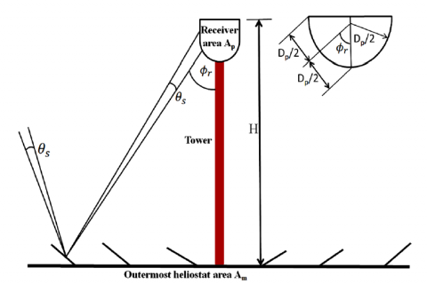
For the analysis of the central receiver collector, first of all, considering the N number of mirrors having the area of Am (1x1= 1 m2) and the width is w that covering the ground area Ag around the central tower. In the present work a total of 7 & 9 reflecting mirrors have been used for the calculation of ground area. The value of fraction for the ground area covered is 0.4 [SP. Sukhatmne 2008]. Remember that the placement of the mirrors must prevent incident or reflected radiation from one heliostat from being blocked by another heliostat, as shown in Figure 3.
$N A_m=\psi A_g$ (1)
Calculation of area of ground
$\begin{aligned}& A_g \text { for } \mathrm{N}=7,\left(7 \times 1=0.4 A_g\right) \\& A_g=17.5 \mathrm{~m}^2\end{aligned}$
Calculation of area of ground $A_g$ for $\mathrm{N}=9$
$\begin{aligned}& 9 \times 1=0.38 A_g \\& A_g=22.5 \mathrm{~m}^2\end{aligned}$
In the present work spiral tube is chosen for the focal point 0.6 m*0.6 m with tube diameter 10 mm and gap between each turn is 6 mm, the spiral tube has a total of 16 twists and measures 13.8 meters in length, the heat transfer fluid is water and tube material is copper and have been utilized for the calculation. It is assumed that the receiver is mounted at 1.8 m height and the farthest mirror is 10.8 meters away [SP digole 2020].
Figure 3. Central Power receiver System [1]
3.2 Calculation of size of the image $L_i$ at the absorber
$L_i=\frac{H}{\cos \phi_r}\left(\theta_s+\theta_e\right)+w$ (2)
Where $L_i$ is the size of the image formed by the outermost mirror at the receiver, $\theta_s$ is earth sun angle $\left(0.53^{\circ}\right)(0.00925$ $\mathrm{rad}), H$ is the tower height, $w$ is diameter of mirror, $\theta_e$ is the total angular error associated with the reflection due to factors like mirror surface imperfections and mirror orientation $(0.002$ $\mathrm{rad})$ and $\phi_r=$ is rim angle.
The rim angle can be calculated as:
$\begin{gathered}\phi_r=\cos ^{-1}\left(\frac{H}{\text { distance between the outermost mirror }}\right) =80.4^{\circ} \text { and the receiver }\end{gathered}$
And the Length of the image due to the mirror span $L_i=1.0211 \mathrm{~m}$
3.3 The concentration ratio
$C=\frac{N A_m}{A_p}$ (3)
$C=\frac{N A_m}{\frac{\pi}{2}\left[L_i\right]^2\left(1+\sin \phi_r-\frac{\cos \phi_r}{2}\right)}$ (4)
or
$C=\frac{\psi \pi H^2 \cdot \tan ^2 \phi_r}{\frac{\pi}{2}\left[L_i\right\}^2\left(1+\sin \phi_r-\frac{\cos \phi_r}{2}\right)}$ (5)
$C=45.77$
3.4 Calculation of solar radiation
The geographical setting of Pune, Maharashtra, India lies within Latitude (18.5187 oN), Longitude (73.8158 oE). The climate of the Pune is subtropical where summer is hot and humid and winter is cool and dry, the average temperature is around 20°C and 28 °C during the day and in the summer, it gets up to 42o, while the Monsoon usually from June to October. May is the highest recorded, December-January is the coldest, and July is the wettest.
$\delta=23.45 \sin \left[\frac{360}{365}(284+n)\right]$ (6)
$\omega=$ hour angle $\omega=\cos ^{-1}[-\tan \emptyset \cdot \tan \delta]$ (7)
Table 1. Estimated declination angle, sunshine hour and monthly average radiations at Pune, India
|
Months |
Declination Angle (δ) |
Sunshine Hour Smax |
Monthly avg. Radiation Ho [KJ/m2-day] |
Monthly avg. Beam Radiation Hb [KJ/m2- day] |
|
Jan |
-20.92 |
11.019 |
27723.09 |
21012.61 |
|
Feb |
-12.95 |
11.411 |
31338.93 |
21302.36 |
|
Mar |
-2.42 |
11.892 |
35145.31 |
22092.80 |
|
Apr |
9.41 |
12.424 |
37993.33 |
21156.80 |
|
May |
19.03 |
12.885 |
39121.25 |
21277.42 |
|
Jun |
23.39 |
13.111 |
39214.09 |
21486.56 |
|
Jul |
21.18 |
12.994 |
39015.01 |
21674.88 |
|
Aug |
13.45 |
12.613 |
38229.46 |
21569.00 |
|
Sep |
2.22 |
12.099 |
36029.84 |
21053.40 |
|
Oct |
-9.60 |
11.567 |
32334.32 |
20539.92 |
|
Nov |
-18.91 |
11.121 |
28502.2 |
18668.83 |
|
Dec |
-23.05 |
10.907 |
26587.81 |
14767.16 |
Figure 4(a). Estimated declination angle for different solar months at Pune, Maharashtra
The angular displacement of the sun from the plane of the equator of the earth has been shown in the above graph. It has been remarked that on June 21 and Dec 22, the maximum declination angle is ±23.45o while, Figure 4(a) demonstrates that the declination angle is zero on 22 March & 23 September. Due to the tilt of the rotation of earth's axis of along with the revolution of the sun, the declination angle changes seasonally around the sun and estimated using Eq. (6). The average sunshine hour for the year ranges from 10.9 hours in the month of December to 12.9 hours in the month of July for the selected location due to its geographical location (Table 1).
3.5 Incidence beam, Diffuse and Global radiations on horizontal surface under cloudless skies
$I_a=I_b+I_d$ (8)
$I_b=I_{b n} \cos \theta_z$ (9)
$I_{b n}=A \exp \left(-B / \cos \theta_z\right)$ (10)
$I_d=C I_{b n}$ (11)
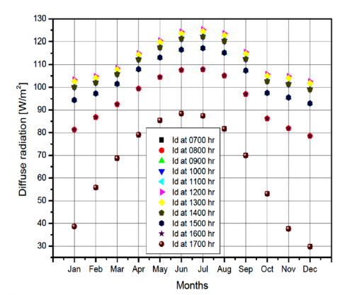
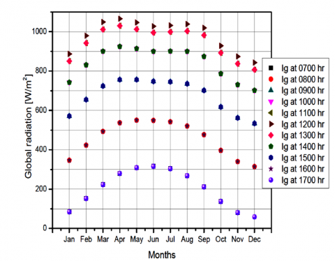
Incidence beam, Diffuse and worldwide radiations on the horizontal plane under cloudless skies have been estimated using Eqs. (9)-(11) with the help of Table 2 for the whole year. The incident beam radiation has been calculated for the solar time 0700 hours to 1700 hours as shown in Figure 4(b). Molecular and particle scattering from the dispersed radiation in the atmosphere estimated and shown in Figure 5 while in Figure 6 the global radiation showed, which the sum of incident and diffused radiation.
Table 2. Constant A, B & C for predicting hourly solar radiation on clear days [SP Sukhatmne 2008]
|
Months |
A (W/m2) |
B |
C |
|
Jan |
1202 |
0.141 |
0.103 |
|
Feb |
1187 |
0.142 |
0.104 |
|
Mar |
1164 |
0.149 |
0.109 |
|
Apr |
1130 |
0.164 |
0.120 |
|
May |
1106 |
0.177 |
0.130 |
|
Jun |
1092 |
0.185 |
0.137 |
|
Jul |
1093 |
0.186 |
0.138 |
|
Aug |
1107 |
0.182 |
0.134 |
|
Sep |
1136 |
0.165 |
0.121 |
|
Oct |
1136 |
0.152 |
0.111 |
|
Nov |
1190 |
0.144 |
0.106 |
|
Dec |
1204 |
0.141 |
0.103 |
Figure 4(b). Estimated beam radiation on horizontal surface for different solar time at Pune, India
3.6 Solar radiation on an inclined plane surface
$I_T=I_b \cdot r_b+I_d \cdot r_d+\left(I_b+I_d\right) r_r$ (12)
$r_b=\frac{\cos \theta}{\cos \theta_z}=\frac{\sin \delta \cdot \sin (\emptyset-\beta)+\cos \delta \cdot \cos \omega \cdot \cos (\emptyset-\beta)}{\sin \emptyset \cdot \sin \delta+\cos \emptyset \cdot \cos \delta \cdot \cos \omega}$ (13)
$r_d=\frac{1+\cos \beta}{2}$ (14)
$r_r=\rho\left(\frac{1-\cos \beta}{2}\right)$ (15)
Figure 5. Diffuse radiation on a horizontal surface as estimated for various sun times at Pune, India
Figure 6. Estimated global radiation on horizontal surface for different solar time at Pune, India
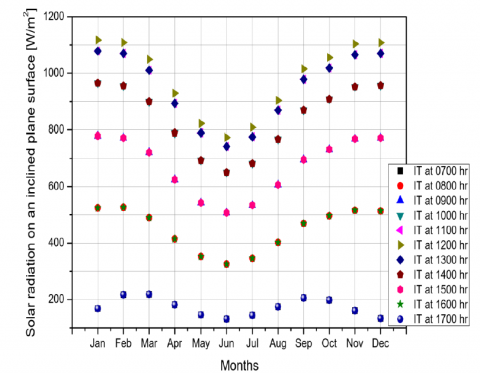
Solar rays hitting an inclination surface have been estimated using Eqs. (12)-(15) with the help of Table 3 for the whole year. The Solar radiation on an inclined plane surface has been calculated for the solar time 0700 hours to 1700 hours as shown in Figure 7.
Table 3. Estimated values of tilt factors at rb, rdandrr Pune, Maharashtra using Eqs. (13)-(15)
|
Months |
Rb at 0700 & 1800 hr |
rb at 1000 & 1800 hr |
rb at 1200 hr |
rd |
rr |
|
Jan |
2.9225 |
1.3344 |
1.2800 |
0.8536 |
0.0293 |
|
Feb |
1.7228 |
1.1577 |
1.1320 |
0.8536 |
0.0293 |
|
Mar |
0.9984 |
0.9846 |
0.9838 |
0.8536 |
0.0293 |
|
Apr |
0.5278 |
0.8207 |
0.8406 |
0.8536 |
0.0293 |
|
May |
0.2863 |
0.7115 |
0.7434 |
0.8536 |
0.0293 |
|
Jun |
0.2052 |
0.6696 |
0.7058 |
0.8536 |
0.0293 |
|
Jul |
0.2787 |
0.7077 |
0.7400 |
0.8536 |
0.0293 |
|
Aug |
0.5224 |
0.8185 |
0.8386 |
0.8536 |
0.0293 |
|
Sep |
0.9885 |
0.9816 |
0.9813 |
0.8536 |
0.0293 |
|
Oct |
1.7712 |
1.1670 |
1.1399 |
0.8536 |
0.0293 |
|
Nov |
2.9835 |
1.3411 |
1.2856 |
0.8536 |
0.0293 |
|
Dec |
3.7327 |
1.4125 |
1.3445 |
0.8536 |
0.0293 |
Figure 7. Estimated solar radiation on an inclined plane surface for different solar time at Pune, India
3.7 Monthly average hourly, beam diffused and global radiation
$\begin{aligned} & H_o=3600 \times \frac{24}{\pi} I_{s c}[1.0+\left.0.033 \cos \left(\frac{360 n}{365}\right)\right]\left(\cos \phi \cos \delta \cos \omega_s+\omega_s \sin \delta \sin \phi\right)\end{aligned}$ (16)
And
$\frac{\bar{H}_g}{\bar{H}_o}=a+b\left(\frac{S}{S_{\max }}\right)$ (17)
Where $S=$ average number of days per month with sunny sunshine and $a \& b$ are the regression parameters for particular location.
For Pune $\mathrm{a}=0.31, \mathrm{~b}=0.43$
$S_{\max }=\left(\frac{2}{15}\right) \omega_s$ (18)
Where Smax= average of the greatest number of hours of bright sunshine per day each month
For Indian conditions where the diffused component is relatively large, the following correlation is used to predict the diffused radiation.
$\frac{\bar{H}_d}{\bar{H}_g}=0.8677-0.7365\left(\frac{s}{s_{\max }}\right)$ (19)
$\overline{\mathrm{H}}_{\mathrm{h}}=\overline{\mathrm{H}}_{\mathrm{o}}-\overline{\mathrm{H}}_{\mathrm{d}}$ (20)
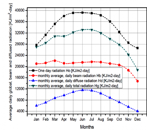
Average daily global, beam and diffused radiation have been estimated using Eqs. (16)-(20) for the whole year and also calculated for the solar time 0700 hours to 1700 hours as shown in Figure 8.
Useful heat gain by considering concentration ratio.
Once the incidence beam radiation and average tilt factors have been known one can compute the useful heat gain using Eq. (21).
$q_u=\psi A_g\left[I_b\left(r_b\right)_{a v} \rho . \tau . \alpha\right]-\frac{U_l}{C}\left(T_{p m}-T_a\right)$ (21)
Figure 8. Estimated average daily global, beam and diffused radiation for different solar month
The following transient equation that relies on the time t and space x, expresses the energy balance of the fluid circulating via the inside tube.
$\begin{aligned} & \rho_{\text {fluid }} \cdot C_{p, f l u i d} \cdot A_{f l u i d} \frac{\partial T_{\text {fluid }}}{\partial t}(x . t)+ \\ & \rho_{\text {fluid }} \cdot C_{p, f l u i d} \cdot \frac{V_{\text {fluid }}}{N_{\text {receiver }}} \cdot \frac{\partial T_{\text {fluid }}}{\partial t}(x . t)=Q_{\text {conv }}(x . t)\end{aligned}$ (22)
Where $\rho_{\text {fluid }}$ is density of fluid, $C_{p \text {,fluid }}$ is specific heat of fluid, $A_{\text {fluid }}$ is area of fluid, $\dot{V}_{\text {fluid }}$ is velocity of the fluid, $N_{\text {receiver }}=$ number of receivers.
Heat transfer by convection between the flowing fluids inside the tube at unit length is:
$Q_{\text {conv }}(x \cdot t)=h_{\text {tube \& fluid }} \cdot A_{\text {receiver }} \cdot\left(T_{\text {receiver }}-T_{\text {fluid }}\right)$ (23)
Where $h_{\text {tube & fluid }}$ is heat transfer coefficient by convection between the tube and the fluid, $A_{\text {receiver }}$ is area of inside surface by length of the tube, $T_{\text {receiver }}$ is temperature of receiver tube and $T_{\text {fluid }}$ is temperature of flowing fluid. The variation of the energy transfer in the heat transfer fluid is written as:
$\frac{\partial T_{\text {fluid }}}{\partial t}(x . t)=\underbrace{\frac{h_{\text {tube & fluid }} \cdot A_{\text {receiver }}}{\rho_{\text {fluid }} \cdot C_{p \text { fluid }} \cdot A_{\text {fluid }}}}_{\alpha_{11}}\left(T_{\text {receiver }}-T_{\text {fluid }}\right)$ (24)
$\frac{\partial T_f}{\partial t}(x . t)=\alpha_{11}\left(T_{\text {receiver }}-T_{\text {fluid }}\right)$ (25)
The above equation is a first-order differential equation describing the variation in fluid temperature as a function of time and the receiver.
4.1 Energy balance for the receiver
$\begin{aligned} & \rho_{\text {receiver }} C_{\text {p,receiver. }} A_{\text {receiver }} \frac{\partial T_{\text {receiver }}}{\partial t}(x . t)=Q_{\text {solar }}(x . t)- \\ & Q_{\text {inlet }}(x . t)-Q_{\text {conv }}(x . t)\end{aligned}$ (26)
Where $Q_{\text {solar }}(x . t)$ represents the amount of solar energy absorbed by the collector or receiver,
$Q_{\text {inlet }}(x . t)$ is the amount of heat transfer at inlet between absorber tube and heat transfer fluid and
$Q_{\text {conv }}(x . t)$ is heat transfer through convection between absorber tube and heat transfer fluid.
$Q_{\text {solar }}(x \cdot t)=I_b \cdot r_b \cdot \tau \cdot \alpha \cdot D_{\text {eff }} \eta_{\text {opt }} \cdot \gamma$ (27)
Where $I_b$ is the incident solar beam irradiance which is calculated for selected location, $r_b$ is tilt factor, $\rho$ is reflectivity $(0.89), \tau$ is transmissivity $(0.9), D_{e f f}$ is the effective width of the receiver, $\eta_{\text {opt }}$ is optical efficiency ( 0.98$)$ and $\gamma$ is the dirt factor on the mirrors $(0.8)$.
4.2 Heat transfer by conduction and radiation between the tube and surrounding
$Q_{\text {inlet }}{ }^{\text {conv }}(x . t)=\frac{2 \pi K_{\text {air }}\left(T_{\text {receiver }}-T_{\text {glass }}\right)}{\ln \left(\frac{R_{\text {tube }, \text { out }}}{R_{\text {tube } \text { in }}}\right)}$ (28)
Where $Q_{\text {inlet }}{ }^{\text {rad }}(x . t)$ the heat is transfer at inlet through radiation and $Q_{\text {inlet }}{ }^{\text {conv }}(x . t)$ is the heat transfer at inlet through convection.
$Q_{\text {inlet }}{ }^{\text {rad }}(x . t)=\sigma \cdot \varepsilon_{\text {tube }} \cdot A_{\text {receiver }}\left(T_{\text {receiver }}{ }^4-T_a{ }^4\right)$ (29)
Where $\sigma$ is Stefan Boltzmann constant $\left(5.67 \times 10^{-8} \mathrm{~W} / \mathrm{m}^2 \mathrm{~K}^4\right)$, $A_{\text {receiver }}$ is inside surface area of the absorber tube throughout of the length and $\varepsilon_{t u b e}$ is emissivity of tube surface.
$Q_{\text {inlet }}{ }^{\text {conv }}(x . t)=\frac{2 \pi K_{\text {air }}\left(T_{\text {receiver }}-T_{\text {glass }}\right)}{\ln \left(\frac{R_{\text {tube }, \text { out }}}{R_{\text {tube }, \text { in }}}\right)}$ (30)
Where $K_{\text {air }}$ is thermal conductivity of air and $R_{\text {tube,in }} \& R_{\text {tube,out }}$ inner and outer radius of the tube.
$\begin{aligned} & Q_{\text {inlet }}(x . t)=\sigma \cdot \varepsilon_{\text {tube }} \cdot A_{\text {receiver }}\left(T_{\text {receiver }}{ }^4-T_a{ }^4\right)+ \\ & \frac{2 \pi K_{\text {air }}\left(T_{\text {receiver }}-T_{\text {glass }}\right)}{\ln \left(\frac{R_{\text {tube }, \text { out }}}{R_{\text {tube } \text { in }}}\right)}\end{aligned}$ (31)
Modeling of the heat transfer equation for the receiver is hard as well as complicated because of large number of variables and parameters. Now it has been tried to formulate the mathematical model for the heat transfer through the receiver as mentioned below.
$\begin{aligned} \rho_{\text {receiver }} C_{p, \text { receiver }} & A_{\text {receiver }} \frac{\partial T_{\text {receiver }}}{\partial t}(x \cdot t) \\ & =I_b \cdot r_b \cdot \tau \cdot \alpha \cdot D_{\text {eff }} \eta_{\text {opt }} \cdot \gamma \\ & -\sigma \cdot \varepsilon_{\text {tube }} \cdot A_{\text {receiver }}\left(T_{\text {receiver }}{ }^4-T_a{ }^4\right) \\ & -\frac{2 \pi K_{\text {air }}\left(T_{\text {receiver }}-T_{\text {glass }}\right)}{\ln \left(\frac{R_{\text {tube } \text { out }}}{R_{\text {tube } \text { in }}}\right)}\end{aligned}$ (32)
Divided by $\rho_{\text {receiver }} C_{p, \text { receiver }} . A_{\text {receiver }}$ on both side
$\begin{aligned} & \frac{\partial T_{\text {receiver }}}{\partial t}(x . t) \\ & =\frac{I_b \cdot r_b \cdot \tau \cdot \alpha \cdot D_{\text {eff }} \eta_{\text {opt }} \cdot \gamma}{\rho_{\text {receiver }} C_{p, \text { receiver }} \cdot A_{\text {receiver }}} \\ & -\frac{\sigma \cdot \varepsilon_{\text {tube }} \cdot A_{\text {receiver }}}{\rho_{\text {receiver }} C_{p, \text { receiver }} \cdot A_{\text {receiver }}}\left(T_{\text {absorber }}{ }^4-T_{\text {glass }}{ }^4\right) \\ & -\frac{2 \pi K_{\text {air }}}{\ln \left(\frac{R_{\text {tube,out }}}{R_{\text {tube,in }}}\right) \rho_{\text {receiver }} C_{p, \text { receiver }} \cdot A_{\text {receiver }}}\left(T_{\text {absorber }}\right. \\ & \left.-T_{\text {glass }}\right)-\frac{h_{\text {tube & fluid }} \cdot A_{\text {receiver }}}{\rho_{\text {receiver }} C_{p, \text { receiver }} \cdot A_{\text {receiver }}}\left(T_{\text {receiver }}-T_{\text {fluid }}\right) \\ & \frac{\partial T_{\text {receiver }}}{\partial t}(x . t)=\underbrace{\frac{I_b \cdot r_b \cdot \tau . \alpha \cdot D_{\text {eff }} \eta_{\text {opt }} \cdot \gamma}{\rho_{\text {receiver }} C_{p, \text { receiver }} \cdot A_{\text {receiver }}}}_\psi+\end{aligned}$
$\underbrace{\frac{h_{\text {tube } \& \text { fluid }} A_{\text {receiver }}}{\rho_{\text {receiver }} C_{p, \text { receiver }} A_{\text {receiver }}}}_{\alpha_{12}} T_{\text {fluid }}-$$(\underbrace{\frac{\sigma . \varepsilon_{\text {tube }} \cdot A_{\text {receiver }}}{\rho_{\text {receiver }} C_{p, \text { receiver }} A_{\text {receiver }}}}_{\alpha_{21}}) T_{\text {receiver }}{ }^4-$$\underbrace{\left(\frac{2 \pi K_{\text {air }}}{\ln \left(\frac{R_{\text {tube,out }}}{R_{\text {tube,in }}}\right) \rho_{\text {receiver }} C_{p, \text { receiver }} A_{\text {receiver }}}+\frac{h_{\text {tube & fluid }} \cdot A_{\text {receiver }}}{\rho_{\text {receiver }} C_{p, \text { receiver }} \cdot A_{\text {receiver }}}\right)}_{\alpha_{22}}) T_{\text {rec }}$$\underbrace{\left(\frac{\sigma \cdot \varepsilon_{\text {tube }} A_{\text {receiver }}}{\rho_{\text {receiver }} C_{p, \text { receiver }}, A_{\text {receiver }}}\right)}_{\alpha_{31}} T_{\text {fluid }}{ }^4+$ $(\underbrace{\frac{2 \pi K_{\text {air }}}{\ln \left(\frac{R_{\text {tube,out }}}{R_{\text {tube,in }}}\right) \rho_{\text {receiver }} C_{\text {peceiver. }} A_{\text {receiver }}}}_{\alpha_{32}}) T_{\text {fluid }}$ (33)
After solving this long theoretical equations, the receiver’s energy balance equation can be written as:
$\begin{aligned} & \frac{\partial T_{\text {receiver }}}{\partial t}(x, t)=\psi+\alpha_{12} \cdot T_{\text {fluid }}-\alpha_{21} \cdot T_{\text {receiver }}{ }^4- \\ & \alpha_{22} \cdot T_{\text {receiver }}+\alpha_{31} \cdot T_{\text {fluid }}{ }^4+\alpha_{32} \cdot T_{\text {fluid }}\end{aligned}$ (34)
The above equation is utilized for the prediction of heat transfer from the receiver by putting characteristic parameters such as emissivity, absorptivity and transmission factors etc.
4.3 Energy balance that transforms solar energy between tube and atmosphere
There are the transformations by conduction and radiation between the air and glass envelope.
$\rho_{\text {tube }} C_{p, t u b e} \cdot A_{\text {tube }} \frac{\partial T_{\text {tube }}}{\partial t}(x . t)=Q_{\text {in }}(x . t)-Q_{\text {out }}(x . t)$ (35)
Where $\rho_{\text {tube }}$ isdensity of tube material, $C_{p, t u b e}$ isspecific heat of tube material, $A_{\text {tube }}$ iscross sectional area of tube, $Q_{i n}(x . t)$ is the heat transfer rate at tube's inlet, and $Q_{\text {out }}(x . t)$ is the heat transfer rate at tube's outlet.
The total thermal energy output by convection and radiation between the tube and the surrounding is the sum of heat transfer rate through radiation from the tube and through convection as written as.
$Q_{\text {out }}(x . t)=Q_{\text {out }}{ }^{\text {rad }}(x . t)+Q_{\text {out }}{ }^{\text {conv }}(x . t)$ (36)
Where $Q_{\text {out }}{ }^{\text {rad }}(x . t)$ is the heat transfer rate through radiation from the tube and $Q_{\text {out }}{ }^{\text {conv }}(x . t)$ is the heat transfer rate through convection from the tube.
$Q_{\text {out }}(x . t)=\sigma \varepsilon_{\text {tube }} \cdot A_{\text {tube }, \text { out }}\left(T_{\text {tube }}{ }^4-T_a{ }^4\right)+$ $\sigma h_{\text {tube,amb }} . A_{\text {tube,out }}\left(T_{\text {tube }}-T_a\right)$ (37)
$\begin{aligned} & \rho_{\text {tube }} C_{p, t u b e} \cdot A_{\text {tube }} \frac{\partial T_{\text {tube }}}{\partial t}(x \cdot t)= \\ & \sigma \cdot \varepsilon_{\text {tube }} \cdot A_{\text {receiver }}\left(T_{\text {receiver }}{ }^4-T_a{ }^4\right)+\frac{2 \pi K_{\text {air }}\left(T_{\text {receiver }}-T_a\right)}{\ln \left(\frac{R_{\text {tube,out }}}{R_{\text {tube,in }}}\right)}- \\ & \sigma \varepsilon_{\text {tube }} \cdot A_{\text {tube,out }}\left(T_{\text {tube }}{ }^4-T_a{ }^4\right)- \\ & \sigma h_{\text {air,amb }} \cdot A_{\text {tube,out }}\left(T_{\text {tube }}-T_a\right)\end{aligned}$ (38)
For creating the partial differential equation for the heat transfer through the tube and surrounding by dividing $: \rho_{\text {tube }} C_{p, t u b e} \cdot A_{\text {tube }}$
$\begin{aligned} & \frac{\partial T_{\text {tube }}}{\partial t}(x . t)=\underbrace{\left(\frac{\sigma \cdot \varepsilon_{\text {tube }} \cdot A_{\text {receiver }}}{\rho_{\text {tube }} C_{p, \text { tube }} \cdot A_{\text {tube }}}\right)}_{\beta_{11}} T_{\text {receiver }}{ }^4+ \\ & \underbrace{\left(\frac{1}{\rho_{\text {tube }} C_{p, \text { tube }} \cdot A_{\text {tube }}}\right)\left(\frac{2 \pi K_{\text {air }}}{\ln \left(\frac{R_{\text {tube }, \text { out }}}{R_{\text {tube,int }}}\right)}\right)}_{\beta_{12}} T_{\text {receiver }}- \\ & \underbrace{\left(\frac{\sigma \cdot \varepsilon_{\text {tube }} \cdot A_{\text {receiver }}}{\rho_{\text {tube }} C_{p, \text { tube }} \cdot A_{\text {tube }}}+\left(\frac{\sigma \cdot A_{\text {tube,out }}}{\rho_{\text {tube }} C_{p, \text { tube }} \cdot A_{\text {tube }}}\right)\right)}_{\beta_{21}} T_a{ }^4+ \\ & \underbrace{\left(\frac{\sigma \varepsilon_{\text {tube }} \cdot A_{\text {tube }, \text { out }}}{\rho_{\text {tube }} C_{p, \text { tube }} \cdot A_{\text {tube }}}+\frac{\sigma \cdot h_{\text {tube }, \text { out }} \cdot A_{\text {tube }, \text { out }}}{\rho_{\text {tube }} C_{p, \text { tube }} \cdot A_{\text {tube }}}\right)}_{\beta_{22}} T_a+ \\ & \underbrace{\left(\frac{\sigma \cdot \varepsilon_{\text {tube }} \cdot A_{\text {tube }, \text { out }}}{\rho_{\text {tube }} C_{p, \text { tube }} \cdot A_{\text {tube }}}\right)}_{\beta_{31}} T_a{ }^4+\underbrace{\left(\frac{\sigma \cdot h_{\text {tube }, a m b} \cdot A_{\text {tube }, o u t}}{\rho_{\text {tube }} c_{p, t u b e} \cdot A_{\text {tube }}}\right)}_{\beta_{32}} T_a \\ & \end{aligned}$ (39)
After solving these long theoretical equations energy balance that transmits solar energy between atmosphere and tube can be written as:
$\begin{aligned} & \frac{\partial T_{\text {glass }}}{\partial t}(x . t)=\beta_{11} T_{\text {receiver }}{ }^4+\beta_{12} T_{\text {receiver }}-\beta_{21} T_{\text {tube }}{ }^4+ \\ & \beta_{22} T_{\text {tube }}+\beta_{31} T_a{ }^4+\beta_{32} T_a\end{aligned}$ (40)
It has been observed from the above equations the parameters $\alpha_{i j}$ and $\beta_{i j}$ are constant depends on the characteristics of the fluid used. From these variables the matrix equation can be formed and can be calculate the energy possessed by the system.
$\begin{aligned} \frac{\partial}{\partial t}\left[\begin{array}{c}T_{\text {fluid }} \\ T_{\text {receiver }} \\ T_a\end{array}\right]=\psi+\left[\begin{array}{ccc}-\alpha_{11} & \alpha_{11} & 0 \\ \alpha_{12} & -\alpha_{22} & \alpha_{32} \\ 0 & \beta_{12} & \beta_{22}\end{array}\right]\left[\begin{array}{c}T_{\text {fluid }} \\ T_{\text {receiver }} \\ T_a\end{array}\right] \\ +\left[\begin{array}{ccc}0 & 0 & 0 \\ 0 & -\alpha_{21} & -\alpha_{31} \\ 0 & \beta_{11} & \beta_{21}\end{array}\right]\left[\begin{array}{c}T_{\text {fluid }}{ }^4 \\ T_{\text {receiver }}{ }^4 \\ T_a{ }^4\end{array}\right] \\ +\beta_{31} T_a{ }^4+\beta_{32} T_a\end{aligned}$ (41)
In the above matrix equation, there are three variables ( $T_{\text {fluid }}, T_{\text {receiver }}, T_a$ ) will use to calculate the energy possess under first order differential equation.
$\begin{aligned} & \frac{\partial}{\partial t}\left[\begin{array}{c}T_{\text {fluid }} \\ T_{\text {receiver }} \\ T_a\end{array}\right] \\ & =0.165 \\ & +\left[\begin{array}{ccc}-(0.0055) & 0.0055 & 0 \\ 0.00733 & -(0.0085) & 0.00117 \\ 0 & 0.00117 & 420.433 \times 10^{-12}\end{array}\right]\left[\begin{array}{c}T_{\text {fluid }} \\ T_{\text {receiver }} \\ T_a\end{array}\right] \\ & +\left[\begin{array}{ccc}0 & 0 & 0 \\ 0 & -\left(4.973 \times 10^{-12}\right) & -\left(4.973 \times 10^{-12}\right) \\ 0 & 4.973 \times 10^{-12} & 9.946 \times 10^{-12}\end{array}\right]\left[\begin{array}{c}T_{\text {fluid }}{ }^4 \\ T_{\text {receiver }}{ }^4 \\ T_a{ }^4\end{array}\right] \\ & +4.973 \times 10^{-12} T_a{ }^4+415.4610^{-12} T_a\end{aligned}$
Thermal efficiency of the central tower solar receiver
$\eta_{\text {th }}=\frac{\text { h.A sur,inner } \cdot\left(\mathrm{T}_{\text {out }}-\mathrm{T}_{\text {in }}\right)}{\mathrm{I}_{\mathrm{b}}}$ (42)
$A_{\text {sur,inner }}=2 \pi \cdot r_{\text {in }} \cdot L$
And Electrical efficiency
$\eta_{e l}=\frac{P_{\text {receiver }}}{G . A_{\text {eff }}}$ (43)
Where $P_{\text {receiver }}$ iselectrical power in the receiver, $A_{\text {eff }}$ is effective area and $G$ is solar irradiation
This article presented the study of a central tower solar receiver which comprises a central tower with a receiver and a number of heliostats around the tower. The major goal of this study is to perform a mathematical analysis of the central tower solar receiver where solar load calculation and heat transfer analysis has been carried out. Solar load is calculated for the location of Pune, Maharashtra, India. Results of the mathematical modeling reveal that the estimated average sunshine hour for the year ranges from 10.9 hours in the month of December to 12.9 hours in the month of July. The maximum incident beam radiation of 1050.9 w/m2 has been estimated in the month of April at 1200 hour. The estimated average daily global, beam and diffused radiation for the different solar months are maximum in the month of May & June.
It has been observed from the mathematical modeling for the heat transfer from the fluid, copper tube and surrounding parameter αij and βij is constant and depend on the characteristics of the fluid & metal used. After calculating the variables, the matrix equation can be formed and calculate the energy possess under first-order differential equation by the system. Once the maximum temperature of the heat transfer fluid, copper tube and ambient air will know one can find the thermal efficiency of the system.
The authors extend their sincere appreciation to Dr.Vishwanath Karad MIT World Peace University, Pune, Maharashtra, India, for allowing us to use their infrastructure and simulation software for this analysis.
|
Do |
outside diameter of the tube |
|
Di |
inside diameter of the tube |
|
L |
length of the tube |
|
Q |
theoretical heat rate |
|
Am |
mirror area (m2) |
|
IB |
solar beam radiation (w/m2) |
|
IG |
global radiation (w/m2) |
|
ID |
diffuse radiation (w/m2) |
|
Qt |
heat absorbed by receiver (W) |
|
Qa |
heat absorbed by working fluid (W) |
|
Qc |
convective losses (W) |
|
QY |
radiation loses (W) |
|
ℎ |
heat transfer coefficient (w/m2 K) |
|
A0 |
the receiver absorber area (m2), |
|
Ta |
the Ambient temperature of air (K) |
|
Tw |
mean temperature of tube surface (K) |
|
T0 |
is the outlet temperature of working fluid (K) |
|
Ti |
the Inlet temperature of working fluid (K), |
|
m |
mass flow rate (Kg/sec) |
|
cp |
specific heat (kJ/Kg k) |
|
$\omega$ |
Hour Angle |
|
$\rho$ |
Density of fluid |
|
$\mathrm{m}$ |
Mass Flow Rate |
|
$\eta_{-}th$ |
Thermal Efficiency |
[1] M. Laporte-Azcu et al. (2021) “Material selection for solar central receiver tubes” Solar Energy Materials & Solar Cells 231 (2021) 111317. https://doi.org/10.1016/j.solmat.2021.111317.
[2] Muhammad TahaManzoo et al. (2021) “Convection in volumetrically absorbing solar thermal receivers: A theoretical study” Solar Energy 224 (2021) 1358–1368. https://doi.org/10.1016/j.solener.2021.06.048
[3] Bhrigu Rishi Mishra et sl. (2020) “Comparison of three models to estimate the slant path atmospheric attenuation in central receiver solar thermal plants under Indian climatic conditions” Solar Energy 211,(2020) 1042–1052. https://doi.org/10.1016/j.solener.2020.10.049.
[4] Madjid Amani & Adel Ghenaiet (2020) “Novel hybridization of solar central receiver system with combined cycle power plant” Energy 201 (2020) 117627 https://doi.org/10.1016/j.energy.2020.117627.
[5] Sanjay N Havaldar et al. (2022) “An experimental study of solar receiver under cloudy weather conditions” IOP Conf. Series: Earth and Environmental Science, 1057 (2022)012010. https://doi.org/10.1088/1755-1315/1057/1/012010 .
[6] D. Chen et al. (2019) “High temperature properties of AlN coatings deposited by chemical vapor deposition for solar central receivers” Surface & Coatings Technology 377 (2019) 124872. https://doi.org/10.1016/j.surfcoat.2019.07.083.
[7] Jiabin Fang et al. (2019) “Numerical investigation of the natural convective heat loss of a solar central cavity receiver with air curtain” Applied Thermal Engineering 152 (2019) 147–159. https://doi.org/10.1016/j.applthermaleng.2019.02.087.
[8] Ayad K. Khlief et al. (2018) “Design a New Receiver for the Central Tower of Solar Energy” MATEC Web of Conferences 225, 02009 (2018) https://doi.org/10.1051/matecconf/201822502009.
[9] Danyela Samaniego Rascon et al. (2018) “Ocular risks assessment in a central receiver solar power facility based on measured data of direct solar radiation” Solar Energy 164 (2018) 77–88. https://doi.org/10.1016/j.solener.2018.02.034.
[10] Andreas Fritsch et al. (2017) “A comparison between transient CFD and FEM simulations of solar central receiver tubes using molten salt and liquid metals” Solar Energy 155 (2017) 259–266. http://doi.org/10.1016/j.solener.2017.06.022.
[11] Danyela Samaniego Rascon et al. (2017) “Cumulative and momentary skin exposures to solar radiation in central receiver solar systems” Energy 21 February 2017, http://doi.org/10.1016/j.energy.2017.02.170.
[12] Jay Prakash Bijarniya et al. “Concentrated solar power technology in India: A review”, Renewable and Sustainable Energy Reviews 63 (2016) 593–603, http://doi.org/10.1016/j.rser.2016.05.064.
[13] DanyelaSamaniegoRascon et al. (2016) “Occupational exposures to solar radiation in concentrated solar power systems: A general framework in central receiver systems” Renewable and Sustainable Energy Reviews 65 (2016) 387–401. http://doi.org/10.1016/j.rser.2016.06.038.
[14] M.A. Reyes-Belmonte et al. (2016) “Optimization of a recompression supercritical carbon dioxide cycle for an innovative central receiver solar power plant” Energy 112 (2016). http://doi.org/10.1016/j.energy.2016.06.013.
[15] Alberto Sanchez-Gonzalez & Domingo Santana (2015) “Solar flux distribution on central receivers: A projection method from analytic function” Renewable Energy 74 (2015) 576e587. http://doi.org/10.1016/j.renene.2014.08.016.
[16] J. Coventry et al. (2015) “A review of sodium receiver technologies for central receiver solar power plants” Solar Energy 122 (2015) 749–762. http://doi.org/10.1016/j.solener.2015.09.023.
[17] Bruno Coelho et al. (2014) “Optimization of an atmospheric air volumetric central receiver system: Impact of solar multiple, storage capacity and control strategy" Renewable Energy 63 (2014), 392e401. http://doi.org/10.1016/j.renene.2013.09.026.
[18] Maria Reyes Rodriguez-Sanchez et al. (2014) “Comparison of simplified heat transfer models and CFD simulations for molten salt external receiver” Applied Thermal Engineering 73 (2014) 993e1005. http://doi.org/10.1016/j.applthermaleng.2014.08.07
[19] J. Pacio& Th. Wetzel (2013) “Assessment of liquid metal technology status and research paths for their use as efficient heat transfer fluids in solar central receiver systems” Solar Energy 93 (2013) 11–22. http://doi.org/10.1016/j.solener.2013.03.025.
[20] Weidong Huang et al. (2013) “Prediction and optimization of the performance of parabolic solar dish concentrator with sphere receiver using analytical function” Renewable Energy 53 (2013) 18-26, http://doi.org/10.1016/j.renene.2012.10.046.
[21] Erminia Leonardi (2012) “Detailed analysis of the solar power collected in a beam-down central receiver system” Solar Energy 86 (2012) 734–745, http://doi.org/10.1016/j.solener.2011.11.017.
[22] Qiang Yu et al. (2012) “Simulation and analysis of the central cavity receiver’s performance of solar thermal power tower plant” Solar Energy 86 (2012) 164–174, http://doi.org/:10.1016/j.solener.2011.09.022.
[23] Sukhatme, S.P. (2008) Solar energy principles of thermal collection and storage. 3rd Edition, Tata McGraw-Hill, Noida, 341.
[24] Sanjay N Havaldar et al. (2022) “Numerical Investigation of Concentrated Solar Central Billboard with Hexagonal Tubes” IOP Conf. Series: Earth and Environmental Science 1084 (2022) 012021, IOP Publishing. https://doi.org/10.1088/1755-1315/1084/1/012021