Geetha G. | Arun Mozhi Selvi Sundarapandi* | Hemlathadhevi A. | Surendran Rajendran
© 2024 The authors. This article is published by IIETA and is licensed under the CC BY 4.0 license (http://creativecommons.org/licenses/by/4.0/).
OPEN ACCESS
The goal of this work is to create a closed-loop control system that combines continuous glucose, carbohydrates, and physiological variable readings to regulate glucose levels to treat hyperglycemia and prevent hypoglycemia, as well as a hypoglycemia early alarm module. We use an Extended Kalman filter (EKF) to estimate time-series coefficients of type 1 diabetic patient's glucose levels using a 4-variate time series data such as glucose level, insulin dose, physical activities, and food consumption. An adaptive Kalman Filter algorithm is best suitable for sensor fusion and also for real-time data, which uses the series of measurement data over the period to tend to predict the unknown variable. We proposed to provide the mealtime bolus as a prolonged bolus, with a slice of the insulin dosage delivered before food and the remainder delivered after food. Our research entails the use of a glucose monitor (CGM), physical activity monitor (accelerometer sensor), carbohydrates monitor (biosensor), an automatic insulin infusion controller that calculates the quantity of insulin to be injected, and an insulin infusion drive. Low-Power and Lossy Routing (LPLR) with 6LoWPAN are proposed for efficient routing and private networks. Our model is evaluated using the UVa/Padova simulator for 25 patients. We conducted our experiments with 25 virtual patients with a mix of all age categories. The simulator's default sample time is one minute, but we have set the 5-minute sampling time. Overall, the proposed models are good at predicting hypoglycaemic (<70 mg/dl), normal glycaemic (>70 and 180 mg/dl), and hyperglycaemic (180 mg/dl) blood sugar levels.
sensors, low-power and lossy routing, optimized closed loop control, glycaemic, hypoglycemia, hyperglycemia
Existing Artificial Pancreases system measures blood glucose concentration levels by extracting information from the CGM sensor, and based on the BGC, the control algorithm implemented in the controller automatically adjusts the insulin infusion rate of the automated insulin delivery system. The probable obstacles to executing an automatic insulin infusion engine contain hypoglycemia conditions, misunderstanding regarding suitable glycemic targets, various system, and procedural issues, and resistance to change. Insulin dosage, food intake, daily activities and lifestyle, and emotional states all have an impact on glucose variations in diabetic individuals. Our body discharges low, basal insulin to keep blood sugar levels under control overnight, fasting, and in the middle of suppertimes. A huge burst of insulin is released when you eat. This burst of insulin is required to eliminate all of the carbohydrates that your meal has taken something in. At mealtimes, a fast burst of insulin is released to manage blood glucose levels while eating. This mealtime insulin surges peak in around 45 minutes and then return to baseline/background levels. Because insulin stimulates glucose uptake by cells, this results in an inability to regulate normal blood glucose levels. Long-standing problems such as neuropathy, heart disease, and diabetes might occur if blood glucose levels continue to be high for a lengthier period. If it is left untreated, it causes Hyperglycaemia as well as chronic multiple organ impairment, cardiovascular disease, kidney failure, and blindness. To treat type 1 diabetes-related comorbidities, proper insulin therapy must be given to the patients at right time.
An AR model depends on only continuous blood glucose data of type-1 diabetic patients; the performance of parameter estimation was evaluated by using data-shooting and regularisation strategies to identify diabetic patients. However, in some studies exogenous (X) input variables can be used to include the special effects of insulin intake or carbohydrate intake on glucose, albeit the effect of carbohydrate intake on glucose is far less studied than the effect of insulin. ARMA models, ARMAX, and ARX models are developed for predicting the blood glucose levels in the existing literature survey [1].
Deep learning algorithms boost the performance of IoT- based healthcare applications dramatically. However, if the training values do not appropriately cover all working circumstances, CNN will be unable to extract useful features. However, it might be a difficult task during emergencies since data may not be available. The work create a new data-driven patients, taking into account the impact of prior glucose measurements, insulin, physical activity, and food intake. To estimate time-varying parameters and a state variable like glucose concentration at the same time, a recursive estimator based on extended Kalman filtering (EKF) is used. EKF also gives prediction covariance errors of glucose concentration and model parameters, which might be utilized to eliminate false hypoglycemia/hyperglycemia warnings and develop more robust control systems.
Diabetes is a major chronic disease problem with major economic and social impacts around the world. There have been no studies to solve the potential of M-IoT. Advanced physiological assessment techniques and non-invasive blood glucose detection for diabetes management are used. In this paper [2, 3], a new type of wireless sensing system for monitoring and analyzing heart conditions is proposed and it is proposed to send information to the Internet of Things applications and caregiver/s and doctors for (IoT) tourism. The proposed [4-6] ECG remote monitoring is devoted to non-technical users who require the Internet of Things (IoT) infrastructure, long-lasting healthy living environment monitoring, and system integration over the wider Internet.
A new device is to be proposed for the first-order (FO) predictive coefficient (PC) differential sensor (DS) [7, 8] and signal quality assurance (SQA). It can significantly reduce false positives. The system will notify you promptly. Disconnection and saturation sensors become the issues during unmonitored health monitoring. In this document [9], it is proposed that devices that can wear bio-sensing masks monitor pain intensity using facial electromyography (surface electromyography). The wearable device can be used as a wireless sensor node and is integrated into a tourist-to-noise ratio system to monitor the IoT for remote pain. In this paper [10], an intelligent home-based platform, iHome's Health Internet with Things, has been proposed and implemented. The platform has been enhanced to include connectivity and compatible device integration and an intelligent medical box (iMedBox) based on an open platform. The sensor area contains a power board for signal acquisition and dispensation, energy supply, and a central board monitor [11] for three sensors and vital signs for battery charging. All components are installed on the human body, convenient for remote health monitoring applications and its design combines rigidity and flexible configuration. Smart Gateway using Computing Fog [12] is proposed for smart home remote patient health monitoring. Plant field monitoring from remote locations facilitates better utilization and crop quality among workers.
Monitoring Framework of IoT Assisted Electrocardiogram (ECG) [13] is proposed for continuous monitoring of cardiovascular health for secure data transmission. Lightweight ECG signal strength analysis presents the Formulation and implementation of automatic classification. The fuzzy mite system (running on a fog server) predicts environmental risks and the risk of transmitting the infection in real time to user health [14]. Environmental risks are taken from the concept of virtual zones and provide updated information elsewhere. People with chronic diseases should monitor their vital signs regularly and repeatedly [15, 16]. Essential measurement of vital signs and physiological functions will be useful. The Android application displayed in the doctor-related system allows him to receive the patient's current status without physicalizing the smartphone's current demographic data [17, 18].
To eliminate frequent finger pricking, a CGM sensor is utilized to measure the diabetic patient's blood glucose level from the interstitial fluid. Because CGM sensors are implanted beneath the skin, they monitor interstitial glucose rather than blood glucose (BG).CGM sensors can be made "smart" by including algorithms that can send out notifications when glucose concentrations are expected to surpass normal range thresholds [19, 20]. To improve the signal-to-noise ratio (SNR) of CGM data, it must be filtered. There will be minor differences in measurement taken from the interstitial fluid and the blood samples, but it will be the same during the steady state phase.
The accelerometer sensor measures the user's current physical activity, such as sitting, sleeping, walking, jogging, and exercising. Based on the meal consumption, a biosensor is utilized to measure the carbs content. Because blood pressure, BMI, and heart rate have such close correlations, three additional sensors have been used to measure them.
3.1 6LoWPAN architecture
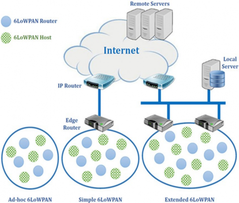
The 6LoWPAN standard enables efficient use of IPv6 at low power through related protocols. An adaptive layer of simple embedded node optimization can be done in low-cost wireless networks. Title Summary is required to operate an effective payload transmission. Also, fragmentation and rearrangement of both transfers should be grouped and layered. Therefore, the MAC network layer is introduced between the adaptive layers. The same IPv6 prefix is distributed by LoWPAN and routers across the LoWPAN node share network interface. The node first uses edge router registration to facilitate efficient network operation. These operations are part of Neighbour Discovery (ND).
Figure 1. 6LoWPAN architecture
However, most of the 6LoWPAN applications such as automatic meter reading and environmental monitoring have been developed using mesh topologies. As it is often covered and cost-effective for infrastructure, it adopts multi-hop forwarding to achieve energy efficiency. Such link-layer meshes, LoWPAN networks, and IPs are done in three different ways, including routing. Link-layer networks and mesh LoWPAN have transparent mesh-mesh transfers and are called the Internet Protocol.
3.2 Low-Power and Lossy Routing (LPLR) with 6LoWPAN
Routing is one of the primary network layer tasks defined in the Open Systems Interconnection (OSI) model. Various other tasks include resolving nodes and creating and maintaining network topologies. 6LoWPAN technology employs a modified IPv6 protocol stack for seamless connectivity. Consider a scalable network of M nodes, let N1, N2, and N3 be the coordinates of each node. A collection point (CP) is considered to be a cluster head at any physical location within it. The network interface of the node can reduce energy usage according to the following parameters.
a) NIC characteristics
b) Packet Size
c) Bandwidth usage
While the node is in listening mode and sleep mode, it assumes energy is being consumed; the power consumption is 1.0 W and 0.001 W respectively.
The transmitted energy and the Joule energy to the received packet are:
$E n_{\text {usage }}=\sum_{\mathrm{j}=1}^{\mathrm{p}} 5 * \operatorname{packetsize}(\mathrm{n}(\mathrm{j}))$ (1)
The lower value of convergence indicates a larger amount of data and the longer time required for training the algorithm. Each solution generates a random path with a maximum number of nodes between the source and destination and satisfies the following constraints.
$N_s \& N_d \leq N_{t h}$ (2)
where, $N_s$ and $N_d$, $\mathrm{s}$ is the source and destination node.
Then it will generate a random path with $N_i$ nodes, let the nodes in this path, $N P_{i+1}$. To evaluate the learning metric $M_p$ of each generated random path:
$M_p=\sum_{i=0}^{N_i} \frac{d_{i-1}}{E(i)}+L S_{i-1}$ (3)
Energy Level of each node $=E$
Link Support $L S_i$
The randomly generated path's learning metrics, i, is a positive integer that takes up the minimum value as two and the maximum value as the total number of nodes in that path, respectively. The $d_{i-1}$ distance between the successive nodes, $E(i)$, is the instantaneous energy of each node right from the source node and $L S_{i-1}$ is the link quality between the successive links in the path.
3.3 Sensor fusion using adaptive Kalman Filte
Let $\mathrm{x}_1, \mathrm{x}_2, \ldots \mathrm{x}_{\mathrm{n}}$ denote the sensor measurements from various sensors with covariance $\mathrm{w}_1, \mathrm{w}_2, \ldots \mathrm{w}_{\mathrm{n}}$ respectively. Each sensor processor $i$ supplies its prior estimates and covariances are $x_i^{\prime}\left(\frac{n+1}{n}\right), w_i^{\prime}\left(\frac{n+1}{n}\right), x_i^{\prime}\left(\frac{n+1}{n+1}\right)$, $w_i^{\prime}\left(\frac{n+1}{n+1}\right)$ where $\mathrm{i}=1,2 . . \mathrm{N}$. Fusion processor prior estimate is $x^{\prime}\left(\frac{n+1}{n}\right), w^{\prime}\left(\frac{n+1}{n}\right)$ and the fusion problem is to compute the total estimates and covariance matrix $w^{\prime}\left(\frac{n+1}{n+1}\right)$.
The Kalman Filter updates or corrects the prediction and the current state's uncertainty after receiving the measurement. The Kalman Filter also forecasts future states and so on. During the prediction step, the system state at the next time stamp is
$X_{n+1, n}^{\prime}=F X_{n, n}^{\prime}+G U_n+W_n$ (4)
where, $\mathrm{G}$ is the control matrix, $\mathrm{U}$ is the input variable, $\mathrm{W}$ is the process noise and $F$ is the state transition matrix. The prediction level of uncertainty is calculated by
$P_{n+1, n}=F P_{n, n} F^{\prime}+Q$ (5)
where, $Q$ is process noise uncertainty $Q_n=E\left(W_n W_n\right)^T$ Initial estimate: $\left(\mathrm{x}_{0,0}^{\prime}, \mathrm{P}_{0,0}\right)$.
During the update step, the Kalman Gain is.
Next, update the system state predicted at time $\mathrm{k}$ by the measured value
$X_{n, n}^{\prime}=X_{n, n-1}^{\prime}+K_n\left(Z_n-H X_{n, n-1}^{\prime}\right)$ (6)
where, output vector $\mathrm{Z}_{\mathrm{n}}=\mathrm{Hx}_{\mathrm{n}}$.
Finally, uncertainty will be updated based on the measurement is:
$P_{n, n}=\left(I-K_n H\right) P_{n, n-1}\left(I-k_n H\right)^T+K_n R_n K_n^T$ (7)
where, measurement uncertainty $R_n=E\left(V_n V_n\right)^T$ Total Daily Insulin Dose (TDID):
Generally, the total insulin required for a day will be calculated based on
$\text { Total daily insulin }=\frac{\text { weights in pounds }}{4}$ (8)
Carbohydrates coverage from the total daily insulin is calculated using the "500" rule by
CarbRatio $=\frac{500}{\text { TDID }}$ (9)
The $BG$ has been quantized into a predetermined number of classes to perform a classification of the events comparable to precise amounts of BG concentration. They are, Severe hyperglycemic, hyperglycemic, normal, hypoglycemic and severe hypoglycemic.
$\begin{gathered}
\text { Class set } C=\left\{\left(\text { if } \emptyset^{\prime}(t)<=50,\right.\right. \text { SHypo), } \\
\text { (if } 50>\emptyset^{\prime}(t)<=70, \text { Hypo), } \\
\text { (if } 70>\emptyset^{\prime}(t)<=180 \text {, Normal), } \\
\text { (if } 180>\emptyset^{\prime}(t)<=250, \text { Hyper), } \\
\text { (if } \left.\emptyset^{\prime}(t)>=250 \text {, SHyper) }\right\}
\end{gathered}$
where, denote the data as $\mathrm{D}_{\mathrm{i}}=\left[\mathrm{BG}_{\mathrm{i}}, \mathrm{HR}_{\mathrm{i}}, \mathrm{BPR}_{\mathrm{i}}, \mathrm{CHO}_{\mathrm{i}}, \mathrm{PH}_{\mathrm{i}}\right.$, $\left.\mathrm{IS}_{\mathrm{i}}, \mathrm{ID}_{\mathrm{i}}\right]$ where all these variables are calculated in the time series from 1 to $\mathrm{n} . \mathrm{BG}_{\mathrm{i}}=\left[\mathrm{BG}_1, \mathrm{BG}_2 \ldots . \mathrm{BG}_{\mathrm{n}}\right]$ is the blood glucose level, $\mathrm{HR}_{\mathrm{i}}$ is the heart rate, $\mathrm{BPR}_{\mathrm{i}}$ is the blood pressure rate, $\mathrm{IS}_{\mathrm{i}}$ insulin boluses, and $\mathrm{ID}_{\mathrm{i}}$ insulin diffusion rate. Typically, a blood glucose level of $180 \mathrm{mg} / \mathrm{dl}$ is typically considered the threshold for hyperglycemia. This value is widely acknowledged as the maximum limit for glucose levels after a meal. This value is crucial in establishing the desired ranges for maintaining glycemic control.
3.4 Estimation of insulin infusion rate from blood glucose concentration using time-varying state model
At time $t$, let $\varnothing^{\prime}(t)$ denote the measured blood glucose level, $x(t)$ denote the insulin delivered, $y(t)$ the carbohydrate being taken and $z(t)$ denotes the energy consumed due to physical activities at time $t$.
The measured blood glucose level at time $\mathrm{t}$:
$\phi^{\prime}(t)=\sigma(t)+n_1(t)$ (10)
$\sigma(\mathrm{t})$ is glucose concentration from interstitial fluid and $\mathrm{n} 1(\mathrm{t})$ is the measurement noise. Measured glucose concentration from the interstitial fluid at time $t+1$
$\sigma(t+1)=\mu_t[\sigma(t)]+I_t[X(t-u)]+M_t[X(t-v)]+\beta(t)$ (11)
$\mu[\sigma(t)]$ is the auto regressive value that denotes the blood glucose values at time $t+1, I_t[x(t-u)]$ is the dynamic linear regression of blood glucose values at time $t+1$ after insulin delivery with $u$ delay, $\mathrm{M}_{\mathrm{t}}[\mathrm{x}(\mathrm{t}-\mathrm{v})]$ is the dynamic linear regression of blood glucose values at time $t+1$ after meal intake with $v$ delay and $\beta(t)$ is the process noise.
$\mu_t[\sigma(t)]=\tau_1(t) \sigma(t)+\tau_2(t) \sigma(t-1)+\ldots+\tau_n(t) \sigma(t-n-1)$ (12)
$I_t[x(t-u)]=\phi_1(t) X(t-u)+\phi_2(t) X(t-u-1)+\ldots+\phi_h(t) X(t-u-(n-1))$ (13)
$M_1[X(t-v)]=\theta_1(t) X(t-v)+\theta_2(t) X(t-v-1)+\ldots+\theta_n(t) X(t-v-(n-1))$ (14)
$\tau_n(t)$ is the auto regressive coefficient, $\varphi_n(t)$ and $\theta_n(t)$ are the linear regression coefficients which are time varying coefficients. $\varphi_n$ will be considered negative because insulin intake always decreases the blood glucose concentration level whereas $\theta_{\mathrm{n}}$ will be assumed to be positive as carbohydrates always increase the blood glucose concentration level
$\left.\phi(t+1)=\frac{d}{d t}[\phi(t+1)+\phi(t)]+[e(t+1)-e(t)]+\left[p(t+1)-p(t)+X\left(t-d_1\right)\right]\right)$ (15)
where,
$\varnothing(t)$ and $\varnothing(t+1)$ is the blood glucose level at time $t$ and $t+1$.
$e(t)$ and $e(t+1)$ is the measurement noise at time $t$ and $t+1$.
$p(t)$ and $p(t+1)$ is the process noise at time $t$ and $t+1$ with zero mean and variance equal to $\sigma^2$.
The formula to determine the insulin dose for high blood glucose levels is:
Insulin dose for high blood glucose=Difference between actual blood sugar and target blood sugar $\div$ correction factor.
$I_h=\frac{\left(\phi^{\prime}(t)-T^{\prime}(t)\right)}{C F}$ (16)
The high blood sugar correction factor is calculated using the "1800" rule by the following formula:
Correction Factor $=\frac{1800}{\text { TDID }}$ (17)
where, TDID is the total daily insulin dose.
3.5 Carbohydrates prediction from the meals
The experiment will then be repeated for the entire day, with varying meal start times, maximum meal sizes, and delays. The projected rise in glucose content $G^{\prime}$ after meal consumption is compared to the observed glucose G". The rate of glucose production at time $t$ is related to the rate of carbohydrate consumption during the meal.
If $M_{s t}$ is the meal's start time, $M_{e t}$ is the meal's finish time, $M_{c g}$ is the meal's carbohydrate content in grams, and $M_d$ is the meal's duration, then $\mathrm{M}=\left[\mathrm{M}_{\mathrm{st}}, \mathrm{M}_{\mathrm{et}}, \mathrm{M}_{\mathrm{cg}}, \mathrm{M}_{\mathrm{d}}\right]$. The maximum meal duration is $\mathrm{M}_{\mathrm{m}}$, and the maximum meal size is $\mathrm{M}_{\mathrm{max}} ; \mathrm{d}$ is the maximum delay between the meal ingestion and the divergence of blood glucose into the circulation.
$G^{\prime}(t) \alpha y^{\prime}(t)$ (18)
$\left(G^{\prime}\left[t^{\prime}-t\right]\right)^{\prime}-\left(G^{\prime \prime}\left[t^{\prime}-t\right]\right)^{\prime}>\phi$ (19)
$d_{e u c}=\sqrt{\sum_i^t \frac{\left|G_p(i)-G_o(i)\right|^2}{t-M_{s t}}}$ (20)
Carbohydrate level at time $t$ is measured by:
$y^{\prime}(t)=\sum_{t=1}^n d_{\text {euc}}(t)+d_{\text {euc }}(t-1)+\ldots . .+d_{\text {euc }}(t-n-1)$ (21)
Using this formula, calculate the carbohydrate coverage insulin dose by:
$I_{C H O}=\frac{y^{\prime}(t)}{C H O \text { in grams inclined by } 1 \text { unit of insulin }}$ (22)
where, "CHO in grams inclined by 1 unit of insulin" differs based on the total daily insulin dose per day.
For example, if you eat 50 grams of carbohydrates for the breakfast, then the $\mathrm{CHO}$ insulin dose is calculated by: $50 / 10=5$ units. This means you need 5 units of insulin to maintain the blood glucose level due to carbohydrate inclination.
Total Insulin Dose $\mathrm{Ti}=\mathrm{I}_{\mathrm{h}}+\mathrm{I}_{\mathrm{CHO}}$ (23)
where, $\mathrm{I}_{\mathrm{CHO}}$ is the $\mathrm{CHO}$ insulin dose and $\mathrm{I}_{\mathrm{h}}$ is the Insulin dose for high blood glucose.
3.6 Continuous Glucose Monitoring (CGM) and energy consumption due to physical activities
Maintaining glycemic imbalance during and after physical activity usually necessitates additional carbohydrate intake and/or insulin cuts. If the physical activity duration is greater than 30 to 60 minutes then 10 to 15 grams of carbohydrates must be consumed to prevent hypoglycemia.
For the entire study participants were allowed to participate in physical activity, with examples including running, fitness center, and walking.
Energy spent due to physical activities is measured by:
$p y^{\prime}(t)=\frac{\sum_{t=1}^n p y(t)+p y(t-1)+\ldots+p y(t-n-1)}{n} * 100 \%$ (24)
The total insulin control action is based on:
$I S_{t+1}=\frac{K_n\left(I S(t-1)+\phi^{\prime}(t)+c^{\prime}(t)-p y^{\prime}(t)=e(t)\right)}{C F}-G R$ (25)
where, $\mathrm{K}_{\mathrm{n}}$ is the Kalman gain.
The equation you provided, Energy Consumption $=$ Power $x$ Time, is accurate. To determine the overall energy usage, one must multiply the power consumption of the system by the duration of its operation. This formula is widely used to calculate energy consumption. Need to guarantee the system's autonomy and maximise its utilisation time. The choice of energy system might be diverse. Low-power and energyefficient systems are generally sought for medical devices, particularly those designed for wear or implantation. This may entail the utilisation of batteries, energy harvesting methodologies (such as solar cells or motion harvesting), or even rechargeable systems, contingent upon the specific application. The specific energy system would rely on the power requirements of your gadgets and the required operational period between charging or maintenance.
3.7 Metrics to evaluate the prediction model
The model's prediction capability was computed on the full test dataset on hypoglycemia extremes (<70 mg/dl) and hyperglycaemic extremes (>180 mg/dl) cases and the mean absolute difference (MAD) is computed using Absolute Difference,
$A(t)=\frac{(\operatorname{CGM}(t) \text { predict }-\operatorname{CGM}(t) \text { actual })}{\operatorname{CGM}(\mathrm{t}) \text { actual }}$ (26)
Mean $A b s o l u t e$ Difference $\operatorname{MAD}(t)=\frac{A(t)}{N}$ (27)
$\operatorname{CGM}(\mathrm{t})_{\text {predict }}$ is the model's predicted glucose value at time $t$, and $\operatorname{CGM}_{\text {actual }}(t)$ is the actual CGM data value at time $t . N$ is the number of data points in the dataset.
Concerning the measured value, relative-absolute change RAC calculates the normalized absolute error between measurement and prediction.
$R A C=\frac{y_i-y^{\prime}}{y_i} * 100 \%$ (28)
The metric used to assess glucose prediction is temporal gain (TG), which represents the amount of average time gained for early identification of a probable hypo/hyperglycemia event using the model.
Temporal Gain $\left(T_{\mathrm{G}}\right)=(\mathrm{n}$-Delay $) * \mathrm{~s}(\mathrm{t})$
$\text { Delay }=\arg \min _{k \in[0,1]}\left\{\frac{1}{n-l} \sum_{i=1}^{n-l}\left(y_i-y^{\prime}\right)^2\right\}$ (29)
where, $\mathrm{n}$ is the number of samples in the dataset, $\mathrm{s}(\mathrm{t})$ is the sampling time.
In our simulations, to find how the meals affect glucose concentrations, we use the simulator's 2-day scenario, which mimics each virtual subject's blood glucose variation for 24 hours, commencing at midnight and ending at midnight, with a breakfast of 50 g of carbohydrate delivered at 7 a.m., 75 g lunch at noon, 7 g snack at 4 p.m., and 50 g for dinner at 8 p.m.. We conducted our experiments with 25 virtual patients with a mix of all age categories. The simulator's default sample time is one minute, but we have set the 5 -minute sampling time. Overall, the proposed models are good at predicting normal (>70 and 180 mg/dl), hypoglycemic (<70 mg/dl), and hyperglycaemic (180 mg/dl) blood sugar levels. The entire 25- patient dataset consists of 21,400 glucose values, with 2640 CGM values of 70 mg/dl accounting for approximately 12.3% of the dataset and 7561 CGM values of 180 mg/dl accounting for approximately 35.33 percent of the dataset, and 11199 CG values accounting for approximately 35.33 percent of the dataset.
Table 1. Simulation parameter
|
Parameters |
Values |
|
Sensors |
Near-Infrared Spectroscopy, MPS-2000, Maxim’s MAX30100, INA219 |
|
Network Protocol |
TCP, MQTT |
|
Controller |
Arduino |
|
Tools |
Visual framework. |
The simulation parameter has been shown in Table 1. The proposed method has been evaluated for its efficiency of multiple parameters based on various simulation conditions. The proposed IoT-enabled diabetic patient's health monitoring (IoT-DPHM) methods simulation results are as follows and compared to existing Lightweight Secure IoT (LS-IoT), Portable Short Range Wireless Technology (PSRWT) method.
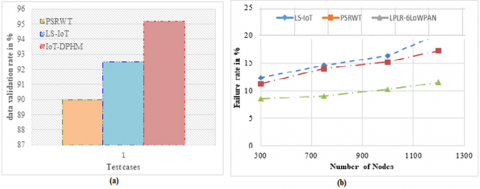
Figure 2. Experimental results (a) Data validation accuracy, (b)
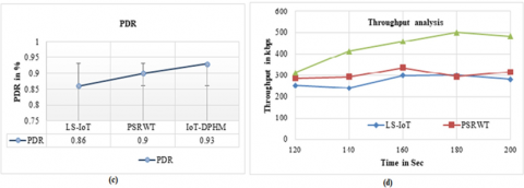
Figure 3. Failure rate, (c) packet delivery ratio, (d)
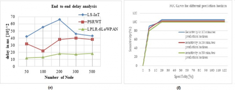
Figure 4. Throughout (e) end to end delay and (f) ROC curve
Figure 2(a) compares the existing methods PSRWT and LSIoT and the proposed method IoT-DPHM method data validation analysis in the IoT network. This proposed IoTDPHM analysis of the data validation has provided a higher performance compared to the existing method. The data prediction failure analysis is challenging to evaluate fault data in this network environment. This proposed failure rate analysis is compared with the existing method which is shown in Figure 2(b). The analysis of proposed IoT-DPHM results shows that the proposed method records an 11.5% or less failure rate compared to other methods, and the existing PSRWT and LS-IoT methods have a higher failure rate. Figure 2(c) represents the packet delivery rate of those initially proposed works. It suggests that the proposed IoT-DPHM is more efficient in data delivery than allPSRWT and LS-IoT. The proposed IoT-enabled diabetic patient's health monitoring (IoT-DPHM) method used Low-Power and Lossy Routing (LPLR) with 6LoWPAN transmitting the data using the IPV6 address. It achieves greater packet distribution over a sensor network. The throughput performance produced by PSRWT and LS-IoT and LPLR-6LoWPAN protocols has been presented in Figure 2(d), where they have produced higher throughput with the normalized value of 498kbps. Figure 2(e) shows the comparison of delay performance of the proposed method LPLR-6LoWPAN, PSRWT, and LS-IoT. In this result, the proposed LPLR-6LoWPANmethod provides an $18.2 * 10^2 \mathrm{~ms}$, and PSRWT provides $38^* 10^2 \mathrm{~ms}$ average time delay performance. The ROC curve is presented in Figure 2(f).
The proposed work developed a closed-loop control system that combines continuous glucose, carbohydrates, and physiological variable readings to regulate glucose levels to treat hyperglycemia and prevent hypoglycemia, as well as a hypoglycemia early alarm module. We have used an extended Kalman filter (EKF) to estimate the time-varying coefficients of type 1 diabetic patient's glucose level using a 4-variate time series of glucose level, insulin dose, physical activities, and meal intake. We conducted our experiments with 25 virtual patients with a mix of all age categories. The simulator's default sample time is one minute, but we have set the 5 minute sampling time. Overall, the proposed models are good at predicting normal (>70 and 180 mg/dl), hypoglycaemic (<70 mg/dl), and hyperglycaemic (180 mg/dl) blood sugar levels. The Cluster-based Time Series Edge Routing for 6LoWPAN is used to collect the data from sensing devices. Low-Power and Lossy Routing (LPLR) with 6LoWPAN have been used to increase the transmission coverage by using an IPV6 modified protocol.
[1] Q. Wang, S. Harsh, P. Molenaar and K. Freeman, “Developing personalized empirical models for Type-I diabetes: An extended Kalman filter approach”, American Control Conference, 2013 DOI:10.1177/1932296814524080
[2] H. Ren, H. Jin, C. Chen, H. Ghayvat and W. Chen, “A Novel Cardiac Auscultation Monitoring System Based on Wireless Sensing for Healthcare”, IEEE Journal of Translational Engineering in Health and Medicine, vol. 6, pp. 1-12, 2018. doi: 10.1109/JTEHM.2018.2847329
[3] M. Bacco , “Monitoring Ancient Buildings: Real Deployment of an IoT System Enhanced by UAVs and Virtual Reality”, IEEE Access, vol. 8, pp. 50131-50148, 2020. DOI: 10.1109/ACCESS.2020.2980359
[4] Z. Zhou, H. Yu and H. Shi, “Human Activity Recognition Based on Improved Bayesian Convolution Network to Analyze Health Care Data Using Wearable IoT Device”, IEEE Access, vol. 8, pp. 86411-86418, 2020. DOI:10.1109/ACCESS.2020.2992584
[5] S. Rani, S. H. Ahmed and S. C. Shah, “Smart Health: A Novel Paradigm to Control the Chikungunya Virus”, IEEE Internet of Things Journal, vol. 6, no. 2, pp. 1306- 1311, 2019. DOI: 10.1109/JIOT.2018.2802898
[6] Palani, V., Alharbi, M., Alshahrani, M. and Rajendran, S., 2023. Pixel Optimization Using Iterative Pixel Compression Algorithm for Complementary Metal Oxide Semiconductor Image Sensors. Traitement du Signal, 40(2). https://doi.org/10.18280/ts.400228
[7] E. Spanò, S. Di Pascoli and G. Iannaccone, “Low-Power Wearable ECG Monitoring System for Multiple-Patient Remote Monitoring”, IEEE Sensors Journal, vol. 16, no. 13, pp. 5452-5462, 2016. 10.1109/JSEN.2016.2564995
[8] H.A. Silva and R. Teresinha, “IoT Applications to Combat 15 Aedes Aegypti: A Systematic Literature Mapping”, IEEE 32nd International Symposium on Computer-Based Medical Systems (CBMS), 2019. 10.1109/CBMS.2019.00141
[9] K.Zhan,”Sports And Health Big Data System Based On 5g Network And Internet Of Things System”, Microprocessors and Microsystems, 2020 https://doi.org/10.1016/j.micpro.2020.103363
[10] U. Satija, B. Ramkumar and M. Sabarimalai Manikandan, “Real-Time Signal Quality-Aware ECG Telemetry System for IoT-Based Health Care Monitoring”, IEEE Internet of Things Journal, vol. 4, no. 3, pp. 815-823, 2017. 10.1109/JIOT.2017.2670022
[11] T. Wu, F. Wu, C. Qiu, J. M. Redouté and M. R. Yuce, “A Rigid-Flex Wearable Health Monitoring Sensor Patch for IoT-Connected Healthcare Applications”, in IEEE Internet of Things Journal, vol. 7, no. 8, pp. 6932-6945, 2020. 10.1109/JIOT.2020.2977164
[12] P. Verma and S. K. Sood, “Fog Assisted-IoT Enabled Patient Health Monitoring in Smart Homes”, in IEEE Internet of Things Journal, vol. 5, no. 3, pp. 1789-1796, 2018. 10.1109/JIOT.2018.2803201
[13] G. Xu, “IoT-Assisted ECG Monitoring Framework With Secure Data Transmission for Health Care Applications”, IEEE Access, vol. 8, pp. 74586-74594, 2020. 10.1109/ACCESS.2020.2988059
[14] S. S. Vedaei , “COVID-SAFE: An IoT-Based System for Automated Health Monitoring and Surveillance in Post- Pandemic Life”, IEEE Access, vol. 8, pp. 188538- 188551,2020. 10.1109/ACCESS.2020.3030194
[15] A. Raji, P. Kanchana Devi, P. Golda Jeyaseeli and N. Balaganesh,, “Respiratory monitoring system for asthma patients based on IoT”, Online International Conference on Green Engineering and Technologies (IC-GET), Coimbatore, pp. 1-6, 2016. 10.1109/GET.2016.7916737
[16] Akshat , “A Smart Healthcare Monitoring System Using Smartphone Interface”, 4th International Conference on Devices, Circuits and Systems (ICDCS), Coimbatore, pp. 228-231, 2018.Bejan, A. (2015). Constructal thermodynamics. Constructal Law & Second Law Conference, Parma, pp. S1-S8. 10.1109/ICDCSyst.2018.8605142
[17] Q. Wang, P. Molenaar, S. Harsh, K. Freeman, J. Xie et al. “Personalized State-space Modeling of Glucose Dynamics for Type 1 Diabetes Using Continuously Monitored Glucose, Insulin Dose, and Meal Intake: An Extended Kalman Filter Approach”, Journal of Diabetes Science and Technology, 2014 https://doi.org/10.1177/193229681452408
[18] Palani, V., Thanarajan, T., Krishnamurthy, A. and Rajendran, S., 2023. Deep Learning Based Compression with Classification Model on CMOS Image Sensors. Traitement du Signal, 40(3), p.1163. https://doi.org/10.18280/ts.400332
[19] Duraisamy, K., Thanarajan, T. and Alharbi, M., 2022. Implementation of Omar Pigeon Space-Time (OPST) Algorithm to Mitigate the Interference and Peak-to- Average Power Ratio (PAPR) Using RPR Mobile and HST-HM in the 5G. Traitement du Signal, 39(5), p.1631. DOI:10.18280/ts.390520
[20] Natarajan, V.P., Thandapani, K. (2021). Adaptive time difference of time of arrival in wireless sensor network routing for enhancing quality of service. Instrumentation Mesure Métrologie, Vol. 20, No. 6, pp. 301-307. https://doi.org/10.18280/i2m.200602