A. Sreenivasulu* | S. Subramanian | P. Sangameswara Raju
© 2023 IIETA. This article is published by IIETA and is licensed under the CC BY 4.0 license (http://creativecommons.org/licenses/by/4.0/).
OPEN ACCESS
Nowadays, the modern world has more concern about increasing population as well as environmental changes. Hence using the Renewable Energy Sources (RES), power generation systems have actively developed in many countries. One of the main sources of RES is solar energy. In solar energy system, emitted energy from the sun is directly converted to electricity in Photovoltaic (PV) system. This research focuses on the advanced techniques based Maximum Power Point Tracking (MPPT) on grid connected and standalone solar PV applications. In this presents the MPPT of standalone solar PV system with Luo converter. Here, to authenticate the performance of the MPPT system with Luo converter, an incremental conductance technique of SPWM and SVM are used. The comparison of Maximum Power Point Tracking of integrated PV system with Sinusoidal Pulse-Width Modulation (SPWM) and Space Vector Pulse Width Modulation (SVPWM) techniques. The SVM performance is greater than the SPWM technique and also SVM technique provides better result than the SPWM. Here, Man of League Algorithm (MLA) is presented for the purpose of preserving the dc voltage of the system.
Maximum Power Point Tracking (MPPT), Photovoltaic, solar cell fuels, Luo converter Space Vector Pulse Width Modulation, Man of League Algorithm (MLA)
Now a days, among the renewable energy power generation systems solar PV is more concentrated in the power generation. Solar PV module directly converts the sunlight into DC power when sunlight falls on PV modules. In many countries, Solar PV power generation plans are executed in very large scales. In the present days, due to the application solar energy such as free, plentiful and pollution free and distributed worldwide, solar photovoltaic (PV) energy is considered as most important available resources. Also, two main problems are in the PV system like low alternative capacity of electric power generation, based on weather condition, the amount of electricity generated by solar panels varies endlessly. Besides, V-I characteristics of the solar cell is nonlinear as well as the irradiation and temperature is varies with this characteristic. Typically, the V-I or V-P curve unique point is known as Maximal Power Point (MPP). The MPP of the PV system provides higher efficiency, as well as generates more productivity throughout the system. The MPP site is unknown, although through computational models or search methods can be traced.
Hence, to maintain the operating point of array at their MPPT (Maximum Power Point Tracking) which techniques are required. The most well-known methods to monitor MPPT are P&O, incremental conductance (INC) method. These methods are updating the operating voltage of array with the duty cycle of power converter with a constant step size. Although solar power is available throughout the day Because of the intensity of the sun on the PV panel, solar irradiation levels vary constantly. This occurs because there are some variations of direct and diffuse radiation of the solar that falls on the solar panel, as well as clouds, birds, trees, etc. These variations produce unpredictable shadows. The general natural intermittence of wind and photovoltaic systems makes their intermediate properties unreliable [1]. Though, by combining the Maximal Power Point Tracking (MPPT) algorithms, the power transfer efficiency and reliability of photovoltaic system can be considerably enhanced, because the operating point of solar panel can be preserved continuously at MPP relative to that radiation and temperature and so on. In this chapter, incremental conductance (INC) method is used for tracking the MPPT as with SPWM and SVPWM technique.
A PV cell forms the PN junction between layers with positively charged P-type material and n-type negatively charged material [2]. This PV cell is like the source of the current from a semiconductor material solar cells are made. If the light is release from the semiconductor some process are occur that are Photo absorption, photo reflection, migration of charge carriers, generation of free carrier charge and finally separation charge by electric fields. The current of solar cell is described by,
$I=I_{S C}-I_O\left[e^{\frac{v}{v_t}}-1\right]$ (1)
Here, short circuit current indicates as $I_{s c}$, saturation current is denoted as $I_o$, voltage across solar cell denoted as ${ }^v$ and thermal voltage denoted as $v_t, k T / q \cong 25.85 \mathrm{mV}$ at room temperature, electron charge denoted as $q$, the value of electron charge is $1.602 \times 10^{-19} \mathrm{C}$, Boltzmann constant denoted as $k$ and its value is $1.38 \times 10^{-23} \mathrm{~J} / \mathrm{K}$, and temperature denoted $\mathrm{as}^t$.
When the voltage is open circuit then the current become zero, therefore no current passing through cell. At same time, open circuit voltage also zero. Applying the conditions of open circuit voltage, $I=0$ and $V=V_{o c}$ then obtain the voltage of open circuit which is determined by below equation,
$V_{o c}=V_T \ln \left(1+\frac{I_{S C}}{I_O}\right)$ (2)
Arithmetically, the voltage obtained from open circuit is large compared to the short circuit. Using the determination, the open circuit voltage is depending on irradiation of the sun. If $I_{s c}=a J_{s c}$ and $I_o=a J_o$ then the open circuit voltage is obtained by,
$V_{O C=} v_t \ln \left(1+\frac{j_{S C}}{j_O}\right)$ (3)
Here, short circuit current density represented as $J_{s c}$, reverse saturation current density is specified as $J_o$, total area of the cell is represented as $a$. The area of cell is independent on open circuit voltage [3]. The outcome of the electrical load as well as the output current supplied to the voltage across the cell is the output power of a solar cell. Electricity has been supplied to the load indicates by positive sign as well as the solar cell is consuming electricity indicates by negative sign. Power supplied at any time is described by,
$\mathrm{P}=\mathrm{V}\left[I_1-I_0\left(e^{\frac{v}{v_t}}-1\right)\right]$ (4)
Among the open circuit and short circuit points of system the maximum power is produced. This point is called as maximal power point in which $V=V_{\operatorname{Max}}$ and $I=I_{M a x}$. When the power becomes zero then the maximum power is also zero. Then the equation becomes,
$\frac{d_p}{d_v}=0=I_I-I_O\left(e^{\frac{V_{\operatorname{Max}}}{v_t}}-1\right)-\frac{V_{\operatorname{Max}}}{v_t} I_O e^{\frac{V_{\operatorname{Max}}}{v_t}}$ (5)
At the point of MPP, maximum current is inclined by,
$I_{M a x}=I_I-I_O\left(e^{\frac{V_{M a x}}{v_t}}-1\right)$ (6)
At the point of MPP, maximum voltage is inclined by,
$V_{\text {Max }}=V_{o c}-V_t \ln \left(1+\frac{V_{\text {Max }}}{v_t}\right)$ (7)
Maximum voltage ( $V_{M a x}$ ) is calculated from the open circuit voltage is known. Different considerations are taken to get the maximum voltage due to the solar cell issue under the change of atmosphere. Then $V_{o c}$ is the maximal voltage variation among cells of forward biased sweep on power quadrant. When the $V_{o c} * V_{M a x}$ for forward biased power quadrant then open circuit voltage may be denoted as,
$V_{o c}=\frac{A k T_{c e l l}}{\mathrm{q}} \ln \frac{I_{P V}}{I_{S a t}}$ (8)
The light generated current is represented as $I_{P V}$, the saturation or leakage current of diode represented as $I_{\text {Sat }}$, electron charge specified as $q$, the Boltzmann constant denoted as $k$, the cell operating temperature specified as $T_{\text {cell }}$ $\left({ }^0 K\right)$, the ideality constant of diode is denoted as $A$. Both $k$ and $T_{\text {cell }}$ must have ideal temperature unit, also Celsius or Kelvin. When the MPP is at a maximum towards the active described load,
$P_{\text {Max }}=V_{\text {Max }} \times I_{\text {Max }}$ (9)
Here, the maximum current is denoted as IMax .
The efficiency of a solar cell system is computed by ratio among maximal power and incident light power.
$\mathrm{n}=\frac{P_{\text {Max }}}{p_{\text {inc }}}$ (10)
The solar radiation product of incident light $(G=\lambda / 1000) \mathrm{W}$ $/ \mathrm{m}^2$ as well as solar cell surface area, $\left(S_a\right)$ in $\mathrm{m}^2$ is used to obtain the incident power.
Pinc $=G . S a$ (11)
The filler factor (FF) is used to measure the quality of solar cell. The fill factor is estimated by comparing the maximal power with theoretical power, i.e. the output of the open circuit and short circuit current join together.
$\mathrm{FF}=\frac{P_{M a x}}{V_{O C} I_{S C}}$ (12)
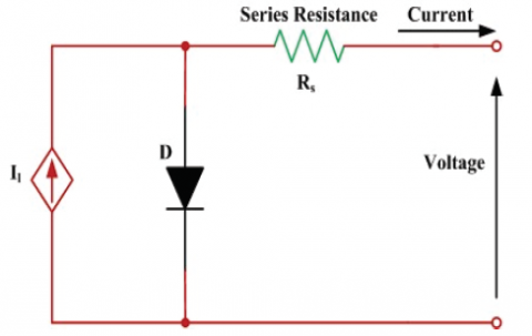
The fill factor depends on the temperature of solar cell. If the temperature of the cell is high then fill factor is low. The range of fill factor is 0.5 to 0.82. In Figure 1 depicts the equivalent circuit of solar cell.
Series Resistance
From solar cell the produced current is transmitting through the base region, which are contacts with resistant semiconductor material generally measured lightly and emitter area generally measured highly. In addition to these components, the metal phase resistance, connections between current collecting buses contribute toward total series resistance losses. The resistance losses are specified through a lumped resistor $R_s$.
Shunt Resistance
Usually the product of large volumes of scales or large parts of thin film products is the solar cell technology used in industry. Factors that contribute to the built-in resistance $R_{s h}$ of the shunt are localized shorts or perimeter shunt at the cell boundary in emitter layer.
Figure 1. Equivalent circuit of solar cell
The space charge region is reorganization which supply to non-ohmic current paths parallel to internal solar cell. This is especially important on minimum voltage dependencies and is referred to as the second diode with the current density of the envelop [4]. The new relationship of current and voltage of the system is obtained from the above effects which is represented as follows,
$I=I_I-I_O\left(e^{\frac{\mathrm{v}+I_{R S}}{n v_t}}\right)-I_{c d}\left(e^{\frac{\mathrm{v}+I R_{s h}}{2 v_t}}\right)-\frac{\mathrm{v}+I R_S}{R_{s h}}$ (13)
2.1 Solar radiation
For analysing the solar cell consider the solar parameters like sun to expose light, temperature, sunlight properties and dust etc. In the surface Sunlight is a radioactive phenomenon per unit area which is expressed in terms of W/m2.Electromagnetic energy of the flow rate is known as Radiation energy. The open circuit voltage remains constant at the exposure which varies favourably with the solar radiation at the short circuit current [5]. To increase performance, the panel surface should be dry and the dust should be kept at a low temperature. Throughout the day solar radiation can be changed. The photo electric current of solar cell is directly proportionate with isolation.
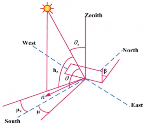
Figure 2 shows the location of the sun at different directions. Depend on the solar radiation the power of the system is achieved. The radiation of solar cell is planned in terms of direct beam irritations, diffuse radiation, direct horizontal radiation, and worldwide radiation [6]. The voltage module must be constant that is the logarithmic function of solar radiation power. The power of that module minimize directly due to the reduction of magnitude of isolation.
Figure 2. Angles Specification to the location of the sun
In Figure 2 , the term $h_z$ is denoted as the zenith angle; $\mathrm{h}$ is referred to as the elevation angle, $l_s$ is denoted as azimuth angle, $l$ is represented by as surface azimuth angle and $\theta$ is represented by angle among the sun and the surface.
The solar radiation energy flux density standing up to the rays at a solid angle on a surface is described as linear beam radiation which is specified as Gn . Linear horizontal radiation Gb differs from linear beam radiation in that it is then projected on a horizontal flat. The horizontal incoming solar radiation with the energy flow density coming from the entire celestial dome surface, excluding the linear beam coming from the sun's disk is called as diffuse radiation Gd total of linearly horizontal and the scattered elements are described as G which means,
Global radiation=linearly radiation+ diffuse radiation (14)
Pyranometer or pyrheliometer is used to calculate the solar radiation. The linearly beam radiation measured by pyrheliometers and the horizontal beam and scattered radiation is measured by pyranometers.
2.2 Effects of the series resistance
In general, the solar cell series resistance has three effects; first one is current flowing through the emitter as well as base of the solar cell. The connection among the resistance through metal and the silicon is the second one. And last one is the resistance top and the metal connections. The target of series resistance is to minimize the fill factor and also minimize short-circuit current. Figure 3 shows that diagrammatic solar cell with series resistance.
Using the above Eq. (13), the short-circuit current may be evaluated as,
$I_{S C}=I_I-I_O\left(e^{\frac{\mathrm{v}+I_{R S}}{n v_t}}\right)-I_{c d}\left(e^{\frac{\mathrm{v}+I R_{S h}}{2 v_t}}\right)-\frac{\mathrm{v}+I R_S}{R_{s h}}$ (15)
Figure 3. Diagrammatic solar cell with series resistance
The open circuit voltage should be evaluated from Eq. (13), consider the current I=0
$I=0=I_I-I_O\left(e^{\frac{\mathrm{v}+I_{R S}}{n v_t}}\right)-I_{c d}\left(e^{\frac{\mathrm{v}+I R_{s h}}{2 v_t}}\right)-\frac{\mathrm{v}+I R_S}{R_{s h}}$ (16)
2.3 Effects of the shunt resistance
Based on the production issues or poor cell modelling the shunt resistance is caused by the power losses. Due to low shunt resistance the power losses is occur in the solar cells which provides an alternative current to light output. This effect can diminish the amount of current flow through solar junction as well as diminishes the voltage as solar cell. Because of low light producing current leads to shunt resistance at low light levels is mostly severe.
Figure 4 shows the diagrammatic of a solar cell shunt resistance. To segregate these causes from others, the second diode and the series resistance is eliminated by using Eq. (13) to setting Rs is a very small value.
Figure 4. Diagrammatic of a solar cell shunt Resistance
2.4 Effects of recombination diode
The recombination diode is an important factor as the fill factor and open circuit voltage are degraded. By p-n junction carriers eradicate each other means the rearrangement of electrons and holes. The electrons are occupied by one or more steps a vacuum attached to a hole.
Figure 5. Irradiative recombination process p-n Junction diode
The p-n junction carriers finally evaporate the operation. Difference among the initial and final state energy of electrons is discharged from the operation. This leads to be an assortment of recombination operation. In the envelope of irradiation recombination, energy is emitted due to the photon. Figure 5 depicts the irradiative recombination process of p-n junction diode.
2.5 Effects of temperature
In the electrical response of the solar cell processing temperature is a great effect. For designing the temperature coefficient electrical boundary is an important factor [7].The great dependence on a temperature has a reverse saturation density current of a diode is inclined by,
$J_0=\mathrm{v} T^{X T_1} e^{\frac{e g}{K T}}$ (17)
Here, constant as well as independent of temperature is denoted as $\mathrm{v}$, the band gap energy of the semiconductor is specified as $e_g$ and the power parameter is denoted as $X T_1$, and it is also the temperature independent. To a reference or nominal temperature $\mathrm{T}$ is inclined by,
$\mathrm{J}_{\mathrm{O}}\left(T_{\text {Ref }}\right)=v T_{R e f} e^{\frac{e_g T_{\text {Ref }}}{K T_{\text {Ref }}}}$ (18)
By dividing the Eqs. (17) and (18) then obtain the equation as follows,
$\ln \left(\frac{J_o}{J_o\left(T_{R e f}\right)}\right)=X T_1\left(\frac{T}{T_{R e f}}\right)+\frac{e_g\left(T_{R e f}\right)}{K T_{R e f}}-\frac{e_g}{K T}$ (19)
Energy band gap of the semiconductor $e_g$ at temperature $T$ rate specified by,
$e_g(T)=e_g(0)-\frac{\operatorname{Gap}_1 \cdot T^2}{\operatorname{Gap}_2+T}$ (20)
The energy band gap is extrapolated by $E_g(0)$ and $T=0^{\circ} \mathrm{K}$ in which the temperature of semiconductor is calculated. Consider the open circuit voltage then the temperature is calculated by,
$\frac{d V_{o C}}{\mathrm{dT}}=\frac{v_t}{\mathrm{~T}} \ln \frac{J_{S C}}{J_0}+v_t \frac{\mathrm{d}}{\mathrm{dT}}\left(\ln \frac{J_{S C}}{J_0}\right)$ (21)
Consider the temperature is independent of short-circuit current then the above equation become,
$\frac{d V_{O C}}{\mathrm{dT}}=\frac{v_t}{\mathrm{~T}} \ln \frac{J_{S C}}{J_0}+v_t \frac{\mathrm{d}}{\mathrm{dT}}\left(\ln J_O\right)$ (22)
Using the Eq. (16), the reverse saturation current density $J_o$ is written as,
$J_O=\mathrm{ET}^\omega e^{\frac{e_g(0)}{K T}}$ (23)
Here, $E, \omega$ are the constants and independent of temperature. By implement the above equation,
$V_{O C}=\mathrm{V}_{\mathrm{t} \ln }\left(1+\frac{J_{S C}}{J_O}\right) \cong V_t \ln \left[\frac{J_{S C}}{J_O}\right]$ (24)
Then the simplification take place, the open circuit voltage is written as,
$\frac{d V_{O C}}{d T}=\frac{V_{O C}}{T}-\frac{\omega N_t}{T}-\frac{e_g(0)}{q T}$ (25)
To the purpose of designing of a PV systems, when necessary to simulate the solar cell characteristics and changed temperature and radiation conditions. The characteristics of solar cell depends on series connected resistance and two current sources [8]. The relation between the short circuit current radiations is provided,
$\mathrm{i}_{\mathrm{rad}}=\frac{J_{s c r}}{1000} \mathrm{~F}+\left[\frac{d J_{s c}}{d T}\right]\left(T_{\text {cell }}-T_{\text {ref }}\right)$ (26)
Here, $F$ denote constant, the solar cell operating temperature is denoted as $T_{\text {cell }}$ and the reference temperature is specified as $T_{\text {ref }}$. The second order current source explains the exponent of the solar cell and is explained as,
$\mathrm{i}(\mathrm{gi})=\frac{j_{s c}(\text { area })}{e^{\frac{V_{o c}}{v_t}}-1}\left(e^{\frac{v}{v_t}}-1\right)$ (27)
The same value of radiation at two temperatures for opencircuit voltage temperature coefficient is,
$\left(\frac{\partial V_{o c}}{\partial \mathrm{T}}\right)\left(T_{\text {cell }}-T_{\text {Ref }}\right)=V_t \ln \left(1+\frac{I_{\text {scref }}}{I_o}\right)-V_{\text {ocref }}$ (28)
Here, the reference temperature at open circuit voltage indicates $V_{\text {ocref }}$, and reference temperature at short circuit current indicates $I_{\text {scref }}$, reference temperature is specified as $T_{\text {ref }}$. using the above equation the voltage become,
$V_{o c}=V_{\text {ocref }}+\left(\frac{\partial V_{o c}}{\partial \mathrm{T}}\right)\left(T_{\text {cell }}-T_{\text {Ref }}\right)+V_t\left(\frac{1+\frac{I_{s c}}{I_o}}{1+\frac{I_{s c r e f}}{I_O}}\right)$ (29)
In general, the short-circuit current becomes zero, the number and class of the last Eq. (29) may be eliminated, and the Eq. (28) is given by,
$V_{o c}=V_{\text {ocref }}+\left(\frac{\partial V_{o c}}{\partial \mathrm{T}}\right)\left(T_{\text {cell }}-T_{\text {Ref }}\right)+V_t \ln \left(\frac{I_{s c}}{I_{\text {scref }}}\right)$ (30)
By the cell temperature $\left(T_{\text {cell }}\right) v_t$ is evaluated. Then the series resistance is evaluated by,
$R_s=\frac{V_{o c}}{I_{o c}}-\frac{P_{M a x}}{F F I^2 o c}$ (31)
The fill factor of the system is described by,
$\mathrm{FF}=\frac{V_{O C}-\ln \left(V_{O C}\right.}{1+V_{O C}}$ (32)
Here, $V_{o c}$ is denoted as open circuit volta ge normalized value to thermal potential $v_t$. To the MPP, the equations for voltage $V_{\text {Max }}$ and current $I_{\text {Max }}$ for arbitrary rate of radiation and temperature can be generated, while employing the following equations,
$I_{M a x}=I_{S c}-I_O\left(e^{\frac{V_{M a x}+I_{M a x} R_S}{v_t}}-1\right)$ (33)
and then maximum voltage is written as
$V_{\text {Max }}=V_t \ln \left(1+\frac{I_{s c}-I_{M a x}}{I_{s c}}\left(e^{\frac{V_{o c}}{v_t}}-1\right)\right)-I_{M a x} R_s$ (34)
2.6 Necessity of MPPT
Practically, photovoltaic systems with lacking batteries are the most generally used. The uses of Battery-free photovoltaic systems are reliability as well as almost maintenance-free, obtain maximal energy performance as solar panels. These systems require particular inverters which are powered by a network that generates reference voltage for its start-up and synchronization using the network. Depend on weather conditions, for getting the maximal power as PV panels; is essential to work with MPPT [9].So, to get the maximal power of system, solar panel inverters are must track the MPP. That provides the system with high efficiency. One of the difficulty tasks in solar system is tracking the maximum power under changing of solar radiation as well as temperature. Furthermore, as solar technology is constantly changing, extensive testing of the actual conditions of different solar modules is nearly not possible.
Figure 6. Maximum Power Tracking of PV system
Figure 6 shows that Maximal Power Tracking of PV system. The volt-ampere characteristic (I–V) of solar cell corresponding point is dependent to select the maximal power point of the system, which is used for increasing the system efficiency.
2.7 SPWM and SVPWM techniques in standalone PV system for tracking MPPT using incremental conductance algorithm (INC)
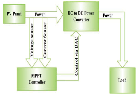
The DC to DC converters such as buck, boost, and buck-boost type are used for converting maximal power to the load as solar cell PV module. The electronic equipment’s are utilized at computer equipment, communication devices, and several control and automation circuits, so on. Figure 7 shows the PV system with converters and the tracking MPPT using INC method. To ensure that PV cells operate on MPP, converters use MPPT techniques. Here, solar system is connected to the luo converter which is used to develop the system output through implementation of MPPT techniques. The proposed system used the INC technique because of its advantages like simple implementation, lesser period to burn up the MPP. The luo converter is connected to the PWM voltage source inverter that is utilized for converting the DC voltage to the AC voltage. Then the filter is connected to voltage source inverter that is used for satisfy the harmonics of system. PI controller is connected to system load. The reference speed is given to the PI controller. From the solar panels, the maximal power point is demonstrated through INC MPPT algorithm in converters is utilized for selecting maximal power point. The SVPWM is the best and most reliable modulation because it enables efficient use of DC voltages and smartly works with vector control thus, gives less Total Harmonic Distortion (THD), better PF, and less switching losses at high frequencies.
Figure 7. Graphic representation of PV system with power converters and INC MPPT tracking
The proposed system contains PV system, luo converter as well as VSC. Using the INC MPPT algorithm, luo converter tracks the PV outcome which is used to achieve the maximum power. The DC current is converted to AC using PWM VSC (DC-AC) converter which is linked to grid or load. System efficiency is described by,
$\eta_{\text {tot }}=\eta_{p v} \cdot \eta_{\text {mppt }} \cdot \eta_{\text {inver }}=\frac{P_{p v}[w]}{G\left[\frac{w}{m^2}\right] \cdot A\left[m^2\right]} \cdot \frac{P_{m p p t}[w]}{P_{p v}[w]} \cdot \frac{P_{o u t}[w]}{P_{m p p t}[w]}$ (35)
Here, $\eta_{\text {tot }}$ total performance of PV system, MPPT algorithm is denoted as $\eta_{\text {mppt }}$, PV inverter is denoted as $\eta_{\text {inver }}$, PV array Efficiency is denoted as $n p v, \mathrm{PV}$ array maximum power is denoted $P_{p v}$.
The proposed solar system consists of 305-WHT panel along 96 cells; furthermore, its capacity is 100 kW in 1000 W / m2, 25°C.
2.7.1 Luo converter (DC-DC converter)
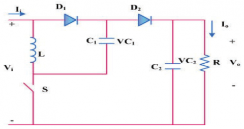
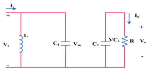
The Luo converter is controlled with INC MPPT algorithm. To achieve maximum DC output voltage capability, the duty ratio is raised or decreased. Figure 9 demonstrates the luo converter equivalent circuit [10]. Through inductance, the current Il passing, therefore the inductance increase the voltage during the period of kT and decreases at (1-k)T . Hence, creating a ripple, inductor current ripple is provided,
$\Delta I_1=\frac{V_{\text {in }}}{L} \mathrm{KT}=\frac{V_0-2 V_{I N}}{L}(1-\mathrm{K}) \mathrm{T}$ (36)
Here, $V_{\text {in }}$ denote as input voltage, $V_0$ denote as output voltage, $k$ denote as duty cycle, $T$ denote as switching time, $L$ denote as inductance value.
Output voltage is provided as,
$\mathrm{V}_0=\frac{2-K}{1-K} \mathrm{~V}_{\text {in }}$ (37)
Voltage transfer gain is described by,
$\mathrm{G}=\frac{V_o}{v_{\text {in }}}=\frac{2-K}{1-K}$ (38)
When the switch is on condition, then the input current is similar with inductor current. While the switch is off condition, the input current is similar with capacitor current. At same time the capacitor current as well as the inductor current is same. The value of the inductor ripple current can be found from the charging and the discharging of the inductor L1[11]. During ON-state, the current through the inductor increases with a slope of $\frac{V_S}{L 1}$ and during OFF-state, it decreases with a slope of $\frac{V_0-2 V_S}{L 1}$.
Figure 8. Luo converter circuit diagram
Figure 9. Luo converter switch on equivalent circuit diagram
Figure 10. Luo converter switch off equivalent circuit diagram
The condition for switching function on, off condition of luo converter is
$I_{\text {in }}(O F F)=I_L(O F F)=I_{C 1}(O F F)$ (39)
$I_{\text {in }}(O N)=I_L(O N)=I_{C 1}(O N)$ (40)
$k T I_{C 1}(O N)=(1-k) T I_{C 1}(O F F)$ (41)
The large inductance current is similar with average current hence current value is,
$I_{\text {in }}(O F F)=I_{C 1}(O F F)=I_{L 1}$ (42)
$\operatorname{Iin}(O N)=I L 1+\left(\frac{1-K}{k}\right) I_{L 1}=\frac{I_{L 1}}{K}$ (43)
$I C 1(O N)=\left(\frac{1-K}{k}\right) I_{L 1}$ (44)
The average input current is described by,
$i_{\text {in }}=k I_{\text {in }}(O N)+(1-k) I_{\text {in }}(O F F)=I_{L 1}+(1-k) I_{L 1}$ (45)
$i_{i n}=(2-k) I_{L 1}$ (46)
The voltage to current ratio is described by,
$\frac{V_{i n}}{I_{i n}}=\left(\frac{1-\mathrm{k}}{2-\mathrm{k}}\right)^2 \frac{V_o}{I_o}=\left(\frac{1-\mathrm{k}}{2-\mathrm{k}}\right)^2 R$ (47)
The output voltage changes is described by
$\delta=\frac{\mathrm{k}}{2 \mathrm{Rf} C_2}$ (48)
Then the output power of the system is
$P o=I o V o$ (49)
Efficiency of the converter is determined by,
$\eta=\frac{P_o}{P_{i n}}$ (50)
2.7.2 Voltage source converter
The voltage source inverter topology uses a diode rectifier that converts AC voltage to DC. The converter is not controlled through electronic firing like the CSI drive. The DC link is parallel capacitors, which regulate the DC bus voltage ripple and store energy for the system. The proposed method used the VSC which convert DC to AC or AC to DC. It contains two current valves which are connected in series manner. The valves consist of semiconductor device and rectifying element. The rectifying element is connected to the parallel manner as well as semiconductor device is locking type. The valves series connection midpoint is linked in the direction of AC side converter.
2.7.3 Incremental conductance algorithm
MPPT approach is a dependable process of INC. The demerits of operational target oscillation $\mathrm{P} \& \mathrm{O}$ practice through MPP among the changing environmental requirements, by increasing PV panel behaviour by increasing instantaneous PV panel behaviour $I_{P V} / V_{P V}$ from INC practice can be improved.
The voltage equivalent with maximum power monitored for satisfying $d P P_{P V} / d V_{P V}=0$, which MPP. The INC installed algorithm is very beneficial through existing traditional approaches as it is simple to realize, high speed and excellent performance. Within this INC MPPT technique, existing and current values of solar voltage and current are realized, so they used for computing value $d I_{P V}$ through $d V_{P V}$. The algorithm of the INC MPPD system used on proposed integrated photovoltaic system is demonstrated at Figure 11.
$\frac{\Delta I}{\Delta \mathrm{V}}+\frac{1}{V}=0$ At MPP (51)
$\frac{\Delta I}{\Delta \mathrm{V}}+\frac{1}{V}>0$ Left of MPP (52)
$\frac{\Delta I}{\Delta \mathrm{V}}+\frac{1}{V}<0$ Right of MPP (53)
Figure 11. Flow chart of INC MPPT algorithm
Figure 12. P-V curve on INC based MPPT System
Figure 12 shows the P–V curve on INC based MPPT system. The INC algorithm is employed to overcome the drawback of P&O algorithm through the PV incremental conductance that is depends on voltage and current value. Depend on the derivative value it can operate and the power at MPP become zero[13]. At the left side of MPP the power value become positive. At the right side of MPP the power value becomes negative. Among the connection of instantaneous conductance (I/V) as well as incremental conductance $(\Delta \mathrm{I} / \Delta \mathrm{V})$ the INC algorithm is processed.
2.7.4 Sinusoidal pulse-width modulation
Pulse width modulation is described by pulse control within fundamental frequency, frequency or width of the pulses is modulated to generate the correct shape of output voltage curve[14]. Generally, PWM used to reduce harmonics of the system.
The PWM output is the change of pulse output width change that is compared to the reference voltage or current through a triangular waveform that has a greater frequency known as carrier. Reference signal is used to modulate the given output whose frequency is similar with fundamental frequency and the harmonics are reduced [15].
Figure 13. Basic block diagram of PWM inverter circuit
Figure 13 shows the basic diagram of PWM inverter circuit. Using the SPWM modulation, the PWM inverter is processing. The AC input voltage is provided with uncontrolled rectifier that gives the DC voltage that can given to the full bridge inverter. The full bridge inverter converts the DC voltage into AC voltage. Hence the PWM inverter circuit also called as AC-DC-AC program. The output of full bride inverter is linked with filter which attenuates the unwanted noise and the output is obtained. The obtained output is feed back to the detecting circuit, using this voltage is isolated and control circuit control the voltage then given to inverter.
2.7.5 Space vector modulation
In the proposed method used the SVM technique based on VSC which is used to achieve the unity power factor as well as permit to attain a sinusoidal input. The SVM has several advantages such as, immediate protection of necessary conversion process, simple algorithm, not including the third harmonic components provides maximum voltage transfer coefficient. Moreover, the proposed switching algorithm minimizes the switching devices concerned at switching process[16]. Therefore, depend on amplitude and phase angle of outcome, the modulation system is directly described. This approach is relevant for highly efficient drive systems.
The result of given system is explained on this portion. For demonstrating the efficiency of approach, the provided method is compared with SPWM as well as SVPWM methods executed on the MATLAB / Simulink work site. PV panel standalone system is taken for the simulation with the tracking of MPPT using the INC approach [17]. To provide the maximum capacity of the modules MPPT is used, which is an electronic system for change the electrical functionality of the modules. Here the efficiency of the system is found by using different speed changes.
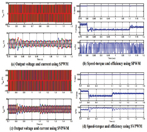
The start up transient response of 3-phase standalone PV system is demonstrated on figure 14. Figure 14(a) portrays that outcome of voltage as well as current using SPWM technique in PV system [18]. The output voltage is varied between -400 to 400V and the time is considered as seconds. The output current of the system is varied between -50 to +50 A. At 0.05 second, the current is varied between -45 to +45 A. At 0.07 sec the current value is reduced to -20 to 20 A. After 0.2 sec the output current of the system is small value i.e around -5 to +5 A. At 0.25 to 0.5 sec the current value is constant. Figure 14 (b) shows the speed torque and performance of system using SPWM. The speed of system is varied in between 0 to 1000 rpm. The speed value is start at 0 sec then it gradually increased to reach 1000 rpm at the time of 0.07sec. Then the speed is constant at 0.07 sec to 0.5 sec. i,e 1000 rpm. The torque value is varied from -25 to +25 Nm. The torque value is start at 0 Nm then increased to 25 Nm at 0.02 sec. Then the torque value at 0.07 sec is varied from -25 Nm to +25 Nm. from 0.22 sec onwards the torque value is around zero that is small changes from zero. The efficiency of the system is varied from 0 to 100 % . At 0 sec the efficiency is 100%. Figure 14 (c) shows the output voltage and current with SVPWM system. The output voltage of the system is varied between -400 to 400Vat the time instant of 0 to 0.5 sec. The current value is changed from -50 to 50 A. From 0.01 sec to 0.05 sec the current value is oscillated between -50 to +50 A. from 0.6 sec onwards the current value is reduced to -20 to 20 A. Figure 14 (d) shows the speed torque as well as performance of system using SVPWM. The speed of the system is varied in between 0 to 1200 rpm. The speed value is start at 0 sec then it gradually increased to reach 1200 rpm at the time of 0.07sec. Then the speed is constant at 0.07 sec to 0.5 sec. i,e 1200 rpm. The torque value is varied from -5 to +15 Nm. The torque value is start at 0 Nm then increased to 15 Nm at 0.02 sec. Then the torque value at 0.07 sec is varied from -25 Nm to +25 Nm. from 0.22 sec onwards the torque value is around zero that is small changes from zero. The efficiency value of the system is varied from 0 to 100%. At 0.01 to 0.04 sec, the efficiency value is 60%. From then the efficiency value is decreased to 60 % at 0.01 to 0.04 sec. From 0.05 sec remains increased to 100%. From 0.12 sec onwards the efficiency value is 100 % i.e constant. Compared the SPWM and the SVPWM technique, the SVPWM technique speed is settled with high efficiency than the SPWM. For instant, at 0.364 sec, torque value is 4.127 Nm as well as efficiency is 95.84 %, In the SVPWM the efficiency is obtained to 98.46 %.
Figure 15 (a) portrays that outcome of voltage as well as current using SPWM technique in PV system. The output voltage is varied between -400 to 400V at the time of 0.4 to 1 sec. After 1 sec the output voltage is zero. The output current of system is varied between 50 to +50 A. At 0.05 second, the current is varied between -45 to +45 A.
After 0.58 sec the output current of the system is small value i.e around 5 to +5 A. At 0.5 sec to 1 sec the current value is constant. Figure 15 (b) shows the speed torque and performance of system using SPWM. The speed of system is varied in between 0 to 1300 rpm. The speed value is start at 0 sec then it gradually increased to reach 1300 rpm at the time of 0.07sec. Then the speed is constant at 0.07 sec to 0.5 sec. i,e 1200 rpm. The torque value is varied from -5 to +15 Nm. From 0 to 0.5 sec, the torque value 0 to 0.2 Nm then it oscillated from -5 to 15 Nm. Then the torque value from 0.6 to 1 sec is varied from 0 to +4 Nm. from 1 sec onwards the torque value is around zero. The efficiency of the system is varied from 0 to 100 % .At 0 sec to 0.5 sec the efficiency is 100%. From 0.5 sec to 0.55 sec the efficiency is varied to 70 %.
Figure 14. Initial-transient response of three-phase standalone PV system
Figure 15. Output voltage and current during servo response with SPWM
Figure 15 (c) shows the output voltage and current using SVPWM system. The output voltage of the system is varied between 400 to 400Vat the time instant of 0 to 1 sec. The current value is changed from -40 to 40 A. From 0.4 sec to 0.5 sec the current value is changed to small value. At 0.5 sec, the current value is oscillated among to -40 to 40 A. Then the current value is small changes from 0. i.e constantly oscillated from 0.55 to 1 sec. Figure 15 (d) shows the speed torque as well as system performance using SVPWM. The speed of system is varied in between 0 to 1400 rpm. The speed value is start at 0 sec then it gradually increased to reach 1400 rpm at the time of 0.086 sec. Then the speed is constant at 0.86 sec to 1 sec. i,e 1400 rpm. The torque value is varied from -5 to +15 Nm. The torque value at 0.4 to 0.5 sec is 0 to 2 Nm then increased to 15 Nm at 0.51 to 0.55 sec.
Figure 16. Speed-torque and efficiency of servo response with decrement of speed 30%using SPWM
Figure 17. Performance of speed-torque and regulation with50%load increment with SPWM
Figure 18. Performance of speed-torque and regulation with75%load reduction with SPWM
Then the torque value at 0.55 sec to 1 sec small oscillation occurs from zero value. The efficiency value of the system is varied from 0 to 100%. At 0.4 to 0.5 sec, the efficiency value is 100%. Then the efficiency value is decreased to 60 % at 0.5 to 0.55 sec. From 0.55 sec it remains increased to 100%. i.e constant. Compared the SPWM and the SVPWM technique, the SVPWM technique speed is settled with high efficiency than the SPWM and the efficiency of SVPWM is 99.47%. The efficiency if SPWM is 98.64%.
The output voltage and current, speed, torque, efficiency at speed increment of 30 % using SPWM and SVPWM. Figure 16 (a) portrays that outcome of voltage as well as current using SPWM technique in PV system. The output voltage is varied between -400 to 400V at the time of 0.4 to 1 sec. At 1 sec to 1.35 sec the output voltage is zero. Then the output voltage is remains varied between -400 to 400V at the time of 1.35 to 1.5 sec. The output current of the system is varied between -45 to +45 A. At 0. 5 sec, the current is varied between -45 to +45 A. After 0.58 sec to 1 sec the output current of the system is small value i.e around -5 to +5 A. From 1 sec to 1.35 sec the current value is oscillating between -5to 5 sec. Figure 16 (b) portrays that speed torque and efficiency of system using SPWM. The speed of the system is varied in between 0 to 1400 rpm. The speed value is start at 0 sec then it gradually increased to reach 1400 rpm at the time of 0.52 sec. Then the speed is constant at 0.52 sec to 1 sec. i,e 1400 rpm. The torque value is varied from -5 to +15 Nm at 0.52 to 0.55 sec. From 0 to 1 sec, the torque value is varied 0 to 0.2 Nm then it became zero at 1 to 1.4 sec. Then the torque value 1.4 to 1.5 sec is varied from 0 to +4 Nm. The efficiency of the system is varied from 0 to 100 % .At 0 sec to 0.5 sec the efficiency is 100%. From 0.5 sec to 0.55 sec the efficiency is varied to 70 %. Figure 16 (c) illustrates that output voltage and current with SVPWM system. The output voltage varied between -400 to 400V at the time of 0.4 to 1 sec. At 1 sec to 1.35 sec the output voltage is zero. Then output voltage is remains varied between -400 to 400V at the time of 1.35 to 1.5 sec. The output current of the system is varied between -45 to +45 A. At 0. 5 sec, the current is varied between -45 to +45 A. After 0.58 sec to 1 sec the output current of the system is small value i.e around -5 to +5 A. From 1 sec to 1.35 sec the current value is oscillate between -5to 5 sec.
Figure 16 (d) shows the speed torque as well as system performance using SVPWM. The speed of system is varied in between 0 to 1400 rpm. The speed value is start at 0 sec then it gradually increased to reach 1400 rpm at the time of 0.52 sec. Then the speed is constant at 0.52 sec to 1 sec. i,e 1400 rpm. The torque value is varied from -5 to +15 Nm at 0.52 to 0.55 sec. From 0 to 1 sec, the torque value is varied 0 to 0.2 Nm then it become zero at 1 to 1.4 sec. Then the torque value 1.4 to 1.5 sec is varied from 0 to +4 Nm. The efficiency of the system is varied from 0 to 100 %. At 0 sec to 0.5 sec the efficiency is 100%. From 0.5 sec to 0.55 sec the efficiency is varied to 70 %. The achieved efficiency of the system using SPWM is 98.45% and the torque is 0.7 Nm.
Figure 17 (a) illustrates that outcome of voltage as well as current using SPWM technique in PV system. The output voltage is varied between -400 to 400V at the time of 0.4 to 0.9 sec. The output current of the system is varied between -20 to +20 A. Figure 17 (b) shows the speed torque and system performance with SPWM. The speed of the system is constant to 1000 rpm at 0.4 to 0.9 sec. The torque value is 10 Nm at 0.4 to 0.5 sec. From 0.5 to 0.8 sec, the torque value is varied 15 Nm then it decreased to 5 Nm at 0.81 to 0.9 sec. The efficiency of the system is varied from 0 to 100 % at 0.4 to 0.9 sec. Figure 17 (c) demonstrates that output voltage and current with SVPWM system. The output voltage is varied between -400 to 400V at the time of 0.4 to 0.9 sec. The output current of the system is varied between -20 to +20 A at 0.4 to 0.5 sec. from 0.51 to 0.8 sec the current value is oscillating between -25 to 25 A. Figure 17 (d) shows the speed torque as well as system performance using SVPWM. The speed of system is constant to 1000 rpm at 0.4 to 0.9 sec. The torque value is 10 Nm at 0.4 to 0.5 sec. From 0.5 to 0.8 sec, the torque value is varied 18 Nm then it decreased to 5 Nm at 0.81 to 0.9 sec. The efficiency of the system is varied from 50 to 99 %. At 0.4 to 0.5 sec, efficiency of the system is 80%. At 0.52 % efficiency is decreased to 50% then it increased to 87% at the time of 0.8 sec. From the analysis the efficiency of the SVPWM technique is high than the SPWM. The output voltage and current, speed, torque, efficiency at speed increment of 75 % using SPWM and SVPWM demonstrated at figure 18. Figure 18 (a) portrays that outcome of voltage as well as current using SPWM technique in PV system. The output voltage is varied between -400 to 400V at the time of 0.7 to 1.5 sec. The output current of the system is varied between -20 to +20 A at 0.7 to 0.8 sec. At 0.8 to 1.1 sec the current value is decreased to -15 to +15 sec. At 1.1 sec to 1.5 sec the current is increased and varied around -20 to 20 A. Figure 18 (b) shows the speed torque and system performance using SPWM. The speed of system is constant to 1000 rpm at 0.75 to 1.2 sec. The torque value is 16 Nm at 0.75 to 0.8 sec. From 0.8 to 1.1 sec, the torque value is 5 Nm then it increased to 10 Nm at 1.1 to 1.5 sec. The efficiency of the system is varied from 50 to 99% at 0.75 to 1.2 sec. Figure 3.18 (c) illustrates that output voltage and current with SVPWM system. The output voltage is varied between -400 to 400V at time 0.7 to 1.5 sec. The output current of the system is varied between 20 to +20 A at 0.7 to 0.8 sec. At 0.8 to 1.1 sec the current value is decreased to -15 to +15 sec. At 1.1 sec to 1.5 sec the current is increased and varied around -20 to 20 A. Figure 18 (d) shows the speed torque as well as system performance using SVPWM. The speed of system is constant to 1000 rpm at 0.7 to 1.5 sec. The torque value is 17 Nm at 0.7 to 0.82 sec. From 0.82 to 1.1 sec, the torque value is 5 Nm then it increased to 10 Nm at 1.1 to 1.5 sec. The efficiency of the system is 75 % at 0.7 to 0.8 sec. At 0.82 sec, the efficiency is reach as 100% then it decreased to 50%. At 0.83 to 1.1 sec the efficiency is 99%.Then it decreased to 80 % at 1.11 to 1.5 sec.
Table 1. Phase as well as Output line to line voltages on SVM technique
|
Volta ge Vecto rs |
Switching Vectors |
Line to neutral voltage |
Line to line voltage |
||||||
|
a |
b |
c |
VAN |
VBN |
VCN |
VAB |
VBC |
VCA |
|
|
V0 |
0 |
0 |
0 |
0 |
0 |
0 |
0 |
0 |
0 |
|
V1 |
1 |
0 |
0 |
2/ |
- |
- |
1 |
0 |
-1 |
|
|
|
|
|
3 |
1/ |
1/ |
|
|
|
|
|
|
|
|
|
3 |
3 |
|
|
|
|
V2 |
1 |
1 |
0 |
1/ |
1/ |
- |
0 |
1 |
-1 |
|
|
|
|
|
3 |
3 |
2/ |
|
|
|
|
|
|
|
|
|
|
3 |
|
|
|
|
V3 |
0 |
1 |
0 |
- |
2/ |
- |
-1 |
1 |
0 |
|
|
|
|
|
1/ |
3 |
1/ |
|
|
|
|
|
|
|
|
3 |
|
3 |
|
|
|
|
V4 |
0 |
1 |
1 |
- |
1/ |
1/ |
-1 |
0 |
1 |
|
|
|
|
|
2/ |
3 |
3 |
|
|
|
|
|
|
|
|
3 |
|
|
|
|
|
|
V5 |
0 |
0 |
1 |
- |
- |
2/ |
0 |
-1 |
1 |
|
|
|
|
|
1/ |
1/ |
3 |
|
|
|
|
|
|
|
|
3 |
3 |
|
|
|
|
|
V6 |
1 |
0 |
1 |
1/ |
- |
1/ |
1 |
-1 |
0 |
|
|
|
|
|
3 |
2/ |
3 |
|
|
|
|
|
|
|
|
|
3 |
|
|
|
|
|
V7 |
1 |
1 |
1 |
0 |
0 |
0 |
0 |
0 |
0 |
VSC phase and line voltage output magnitude on SVM system by seven switching vectors is tabulated in Table 1 . The vector voltages are considered as $\mathrm{V}_0, \mathrm{~V}_1, \mathrm{~V}_2, \mathrm{~V}_3, \mathrm{~V}_4, \mathrm{~V}_5, \mathrm{~V}_6, \mathrm{~V}_7$. Consider the switching vectors $\mathrm{a}, \mathrm{b}, \mathrm{c}$. When the switching vectors become zero than the line to neutral voltage as well as line to line voltage is zero[19]. When the switching vector ", $\mathrm{a}^{\text {a }}$ is on then the line to neutral voltage of VANis $2 / 3, V_{\mathrm{BN}}$ is $1 / 3, \mathrm{~V}_{\mathrm{CN}}$ is $-1 / 3$ and the line to line voltage of $\mathrm{V}_{\mathrm{AB}}$ is $1, \mathrm{~V}_{\mathrm{BC}}$ is zero. $V_{\mathrm{CA}}$ is $-1[20]$. When the switching vector "a" and " $\mathrm{b}$ " is on then the line to neutral voltage of VANis $1 / 3, \mathrm{~V}_{\mathrm{BN}}$ is $1 / 3$, $\mathrm{V}_{\mathrm{CN}}$ is $-2 / 3$ and the line to line voltage of $\mathrm{V}_{\mathrm{AB}}$ is $0, \mathrm{~V}_{\mathrm{BC}}$ is $1, \mathrm{~V}_{\mathrm{CA}}$ is -1.
When the switching vector “b” is on then the line to neutral voltage of VAN is -1/3, VBN is 2/3, VCN is -1/3 and the line to line voltage of VAB is-1, VBC is 1, VCA is 0. When the switching vector “b” and “C” is on then the line to neutral voltage of VAN is -2/3, VBN is 1/3, VCN is 1/3 and the line to line voltage of VAB is-1, VBC is 0, VCA is 1. When the switching vector "c" is on then the line to neutral voltage of VAN is -1/3, VBN is -1/3, VCN is 2/3 and the line to line voltage of VAB is 0, VBC is -1, VCA is 1. When the switching vector “a” and “c” is on then the line to neutral voltage of VAN is -1/3, VBN is -2/3, VCN is 1/3 and the line to line voltage of VAB is 1, VBC is -1, VCA is 0. When all switching vectors are on then the line to neutral voltage of VAN, VBN, VCN become zero as well as line to line voltage of VAB, VBC , VCA become 0.
The study of a three-phase standalone Photovoltaic (PV) system with positive output super-left two DC-DC Converter. The proposed method used two techniques such as SPWM and SVPWM. The system analysed the current, voltage, speed, torque and performance of standalone PV system. When the load is applied the proposed system maximizes the system performance. To ensure that PV cells operate on MPP, converters use MPPT techniques. The solar system is connected to the luo-converter which is used to develop the system output through implementation of MPPT techniques. The luo-converter is utilized for converting the DC voltage into the AC voltage. Then the filter is connected to voltage source inverter that is used for satisfy the harmonics of system. The speed of system enhanced using the proposed method. Also, the cost of the system is minimized by using the proposed method. SVM and SPWM outcome is compared and the SVM performance is greater than the SPWM technique. These two approaches are totally compared and the system performance is evaluated. According to the comparison result, the SVM technique provides better result than the SPWM technique. At last, the SVM technique provides better result than the SPWM is concluded.
[1] Wu TF, Chang CH, Liu ZR, Yu TH. Single-stage converters for Photovoltaic powered lighting systems with MPPT and charging features. In: Proc. IEEE APEC, pp. 1149-1155, 1998.
[2] De BroeAM, Drouilhet S, Gevorgian. V. A peak power tracker for small wind turbines in battery charging applications.IEEE Transactions on Energy Conversion 1999; 14(4): 1630-5.
[3] M. Amelia, S. Moslehpour, and M. Shamlo, Economical load distribution in power networks that include hybrid solar power plants, Elect. Power Syst. Res., vol. 78, no. 7, pp. 1147-1152, 2008.
[4] BahgatABG,HelwabNH,AhmadbGE, ElShe nawybET. Maximumpowerpointtracking controller for PHOTOVOLTAICsystems using neural networks. Renewable Energy 2005;30:1257-68.
[5] SalasV,Oli_asE,BarradoA. ALazaro. Review of the maximum powerpoint tracking algorithms for standalone photovoltaic systems. Solar Energy Materials & Solar Cells 2006;90:1555-78.
[6] EsramT,ChapmanPL. Comparison of photovoltaic array maximum powerpoint tracking techniques. IEEE Transactions on Energy Conversion 2007; 22: 2.
[7] Ali Chermitti, Omar Boukli-Hacene, Bencherif Mohamed Improvement of the Perturb and Observe MPPT Algorithm in PhotovoltaicSystem under Rapidly Changing Climatic Conditions International Journal of Computer Applications (0975-8887) Volume 56-No.12, October 2012.
[8] I.H. Altas; A.M. Sharaf, A Photovoltaic Array Simulation Model for Matlab-Simulink GUI Environment. Proceedings of IEEE, IEEE 2007.
[9] V. Salas, E. Olias, A. Barrado, and A.Lazaro, Review of the maximum power point tracking algorithm for standalone Photovoltaic system, Solar Energy Mater. Solar Cells, vol. 90, no. 11, pp.1555-1578, 2006.
[10] Ahmed K. Abdelsalam, Ahmed M. Massoud, Shehab Ahmed, and Prasad N. Enjeti, High-Performance Adaptive Perturb and Observe MPPT Technique for Photovoltaic-Based Microgrids, IEEE Transactions on Power Electronics, Vol. 26, No. 4, April 2011.
[11] W. Xiao and W. G. Dunford, A modified adaptive hill climbing MPPTmethod for Photovoltaic power systems, in Proc. IEEE 35th Annu.Power Electron. Spec. Conf., Jun. 20-25, 2004, vol. 3, pp. 1957-1963.
[12] G. de Cesare, D. Caputo, and A. Nascetti, Maximum power point tracker for Photovoltaic systems with resistive like load, Solar Energy, vol. 80, no. 8, pp. 982-988, 2006.
[13] V. Salas, E. Olias, A. Lazaro, and A. Barrado, New algorithm using only one variable measurement applied to an MPPT, Solar EnergyMater. Solar Cells, vol. 87, no. 1-4, pp. 675-684, 2005.
[14]. Annam, Sreenivasulu, Subramanian Srikrishna, Sangameswara Raju Prabandhankam, and Ganesan Sivarajan. A Prospective Study on Perturb Observe MPPT Methods for Photovoltaic Systems. Instrumentation,Mesures, Métrologies 22, no. 2 (2023).
[15] F. Liu, Y. Kang, Y. Zhang, and S. Duan, Comparison of p and o and hill climbing MPPT methods for gridconnected PHOTOVOLTAIC generator, in Proc.3rd IEEE Conf. Industrial Electron. Application.,Singapore,Jun.3-5,2008.
[16] Sreenivasulu, A., Subramanian, S., and Sangameswara Raju, P. Design and Simulation of Advanced Intelligent Deep Learning MPPT Approach to Enhance Power Extraction of 1000 W Grid Connected Photovoltaic System. 1 Jan. 2023 : 3987-3998
[17] L. Piegari and R. Rizzo, Adaptive perturb and observe algorithm for Photovoltaic maximum power point tracking, IET Renew. Power Gener., vol.4, no. 4, pp. 317-328, 2010.
[18] N. Femia, D. Granozia, G. Petrone, G. Spagnuolo, andM.Vitelli, Predictive and adaptive MPPT perturb and observe method, IEEE Trans. Aerosp. Electron. Syst., vol. 43, no. 3, pp. 934-950, Jul. 2007.
[19] Y. H. Lim and D. C. Hamill, Simple maximum power point tracker for Photovoltaicarrays, Electron. Lett., vol. 36, no. 11, pp. 997-999,2000
[20] W.XiaoandW. G. Dunford, A modified adaptive hill climbing MPPT method for Photovoltaic power systems, in Proc. 35th Annu. IEEEPower Electron. Conf., Achan, Germany, Oct. 3-7, 2004.