Nagineni Venkata Sireesha | Devineni Gireesh Kumar* | D S N M Rao | Ranjith Kumar Gatla | Sainadh Singh Kshatri | P. Chandra Babu | Bhoopal Neerudi
© 2023 IIETA. This article is published by IIETA and is licensed under the CC BY 4.0 license (http://creativecommons.org/licenses/by/4.0/).
OPEN ACCESS
Fuel cells are now being employed as a source of energy and heat in industrial, transportation, and residential applications. This article presents the real-time implementations and functioning of the proton exchange membrane (PEM) fuel cells. The analysis had been carried out on PEM fuel cells to test the performance systematically and smoothly under transient operations. A change in the current and the resistance of the appliance had been considered for the load variations on PEMFC. This study examined the fuel cell system's efficiency and the time it taken to reach the steady-state without additional means using Artificial intelligence based back propagation network. The proposed analysis proves that the PEM fuel cells which are used for the installations with quickly changing load profiles can provide the improving the system's performance and efficiency.
Fuel cells have grown in importance among sustainable energy generating systems, with applications ranging from residential to industrial to mobile. The most robust and lightweight type of fuel cell is the PEMFC. This type of fuel cell exhibits high performance and durability. Despite the high cost of their membranes and electrodes, the PEMFCs are expected to gain a significant share in the automotive industry in the next few years [1]; similarly, their success in meeting power needs in the built environment appears to be on the rise, particularly as CHP or tri-generation systems [2].
Various thermal and transport mechanisms are also worth investigating in order to improve the efficiency of single-cell and stack response. This is especially true when the system operates under variable load conditions. If the system is run stoichiometrically, then all of the reactants would have to be consumed to generate a certain amount of power. However, this mode is not feasible due to the low partial pressure of these reactants [3, 4].
One of the most common issues that fuel cell developers face is the lack of reactants in the system. To overcome this issue, they can use a flow-through anode. This allows the system to convert unused hydrogen into electricity [5]. Despite the fact that hydrogen losses are reduced in the two systems stated above, several undesirable transport phenomena may occur, affecting system performance. The accumulation of water at the anode causes the concentration of hydrogen to drop. This phenomenon can also affect the flow of hydrogen from the channel to the active reaction sites. Because of these operations, the voltage between the electrodes drops, lowering stack efficiency. Furthermore, the recirculation pump may process crossover gases with unused hydrogen, resulting in a power loss in addition to the voltage drop [6].
For more than a decade, purging both gas and water at the anode outlet prior to gas recirculation has been used and investigated to reduce N2 accumulation and prevent contaminants and, collected water from having a significant influence on stack performance [7]. However, because purging may result in the loss of some hydrogen, some efforts have been made to develop procedures that waste as little fuel as feasible. Their practical application necessitates their integration into the purging-valve control algorithm.
The majority of studies are focused on the dead-end anode mode, with the goal of linking species transport with stack performance, as well as purges in the studied physics. Purging is described as a feature of PEMFC-based CHP devices in several early research, and models that enable analyzing voltage and current density trends from purge-valve opening time and frequency are presented. McKay et al. presented a two-phase flow dynamic model that explains how species concentration across the GDL affects cell voltage and water buildup (Gas Diffusion Layer). Their model will be used to estimate nitrogen and water distributions along anode channels using 1- dimensional methodologies that include periodic purges and calculating N2 accumulation by modeling the permeability of common Nafion membranes [8].
For the past decade, optimizing the purge cycles has been a key topic in the field of engineering. Various studies were conducted to analyze the various aspects of this process, such as the optimal water uptake parameters, the effective purge intervals, and the reduction of hydrogen losses. Experiments have shown that moisture condensation can improve the fuel consumption and purge settings [9, 10]. These studies also linked the various factors that affect the purge cycle to the anode concentration and the humidity.
This research focused on developing an Artificial intelligence based model to predict the operating temperature of a PEMFC. Using experimental data, the model is trained offline. The tracking error of the suggested model is less than 0.5%. It is tested under various settings, and the neural network's operating temperature is established using the experimental data.
The shape of a fuel cell's polarization curve depends on its various operating parameters. A family of these curves can be used to analyze the stack's performance. The higher the parameter variation, the better the polarization curve's performance. This is because it increases the fuel cell's power and improves its electrochemical efficiency [11].
2.1 Impact of pressure on fuel cells
The increasing operating pressure of fuel cells causes the polarization curves to increase. On the other hand, the decrease in operating pressure causes the polarization curves to decrease. The chemical reaction that takes place in a fuel cell depends on the partial pressures of the two components, namely, hydrogen and oxygen. The effects of increasing operating pressure are most prominent when the fuel is used with a dilute oxidant or a reformate [12]. The higher the operating pressure, the more oxygen and hydrogen can be pushed into the electrolyte. This is also the case when the fuel is used at high currents. Although the increase in pressure helps in the electrochemical reaction, it can also introduce other problems. For instance, the flow field plates of fuel cells can suffer from the effects of flowing pressure [13].
When the fuel cell seals are subjected to additional stress, they have to work harder to absorb the additional air compression. This can cause system components to be redesigned. The increasing operating pressure helps in reducing returns. This effect is also beneficial for the overall system. Proton Exchange membrane fuel cells are commonly operated at pressures no higher than a few atmospheres. The use of a pure fuel, which is usually hydrogen or oxygen, can increase the stack polarization curves [14, 15].
2.2 Impact of temperature on fuel cells
The increasing operating temperature affects the fuel cell's polarization curve. On the other hand, the decreasing operating temperature affects the curve.
Some fuel cells can be operated at higher pressures to achieve higher temperatures. This can cause the water boiling point to increase. However, this effect is slight in the case of PEM fuel cells. The higher the operating temperature, the higher the cell's voltage. However, until the temperature reaches the boiling point, the voltage begins to decline. The optimal operating temperature for fuel cells is around 80 degrees Celsius. This temperature is balanced between the two effects [16]. As with high-pressure operations, elevated temperatures can affect various components of the system.
2.3 Impact of stoichiometry on fuel cells
The increase in the reactant gas stoichiometry of fuel cells leads to a decrease in the fuel cell's polarization curve. Insufficient stoichiometry can prevent the fuel cell stack from producing enough reactants. This issue can cause permanent damage to the system. Stoichiometry is a ratio that measures the amount of gas that's needed to complete a reaction. The correct stoichiometric ratio of gas is 1.01. This ensures that the correct number of reactants are produced [17].
For practical fuel cells, the stoichiometric ratios are typically 1.412 and 2.01. However, when operating at low power, higher ratios are required.
2.4 Impact of humidity on fuel cells
A properly humidified gas stream is required for the operation of a fuel cell. This process occurs when hydrogen ions exchange with water molecules. Without sufficient humidification, the water can cause the membrane to get damaged, which can lead to various problems such as cracks and holes. This can also cause a chemical short circuit. When the water gets too humid, it can cause flooding and condensation within the flow field plates, which can destroy the fuel cell. The relative humidity is a measure of the level of moisture in a given gas stream. It can be measured by the temperature and pressure of the gas. A gas that has a relatively high relative humidity level is considered to be saturated. This means that it has a lot of water absorbed by it. When the gas gets hotter, its relative humidity drops. However, if it cools, some of the water condenses, and the gas remains saturated. Ideally, fuel cells should be operated at a temperature that's close to saturated. This ensures that they have enough water to prevent flooding. The use of water for humidification helps limit the operating temperature of a fuel cell to around 0-100 degrees Celsius. Without a continuous flow of water through a demonizing filter, the water can cause corrosion currents and short circuits in the fuel cell stack [18, 19].
A fuel cell is powered by the chemical energy produced by burning hydrogen or other fuels. It then uses this energy to produce electricity. The fuel cells can be used with a wide variety of fuels and feedstocks. They can provide power to various systems, such as a utility power station. Fuel cells are commonly used in various applications, such as transportation and industrial facilities. They can provide reliable and long-term energy storage. Unlike traditional combustion-based technologies, fuel cells have numerous advantages. These include their ability to provide long-term energy storage and reliability [20].
Compared to combustion engines, fuel cells have higher efficiency and lower emissions. They can convert chemical energy into electrical energy, which can reach 60%. They also do not emit greenhouse gases, which are known to contribute to climate change. Unlike other forms of energy, fuel cells do not emit harmful air pollutants during operation. Also, they are quiet during their operation.
The hydrogen consumption during the test was 4 dm3 per minute. To ensure that the fuel cell's supply of hydrogen will remain constant, the researchers added a small amount of overpressure. The stack's control system was powered by a compressor, which allows the cell to receive air through a controlled flow rate. Other components of the system include a hydrogen reducer and a water cooling system. These components regulate the cell's operating temperature and prevent it from overrunning. The control system also monitors the cell's surplus air ratio and the water cooling temperature. It can regulate the cell's operating temperature up to 56 degrees Celsius.
A fuel cell control system is designed to prevent damage to the system while also ensuring its continued operation. This is done through a set of procedures that minimize the risk of failure. The control system must also meet certain constraints to operate efficiently. These include the maximum current, minimum voltage, and cooling water temperature.
If the load exceeds these limits, the control system will automatically disconnect the operation. This prevents the system from working efficiently. Figure 1 shows the various parameters of a fuel cell control system. For optimal operation, it is possible to boost the system's current to 25A and decrease the voltage to 15V for a short period of time.
Figure 1. Fuel cell stack system for the measurement model
The control system for a fuel cell continuously opens the hydrogen outflow valve to improve the efficiency of the fuel cell. This process results in the removal of the fuel cell from its anode side. This process can help regenerate the membrane and remove excess moisture. It can also increase the flow of hydrogen and decrease the inlet pressure of the fuel cell. The heat exchange between the cooling system and the fuel cell is accelerated by the activation of cyclical fans. Maintaining stable operating conditions is very challenging for a fuel cell. This is because its various components and systems can affect its performance [21]. The polarization curve of fuel cell characteristics is shown in Figure 2.
Figure 2. Fuel cell characteristic polarization curve
A schematic diagram of a typical jth node is shown in Figure 3. The inputs to such a node may come from system causal variables (or) outputs of other nodes depending on the layer that the node is located in these inputs form an input vector X=(x1,…xi…xn). The sequence of weights leading to the node form a weight vector Wj = (wij…wij…wnj). Where wij represents the connection weight from the ith node in the preceding layer to jth node.The output of node j, yj is obtained by computing the value of function with respect to the inner product of vector X and w1 minus bj. Where b is the threshold value, also called the bias, associated with this node. In ANN, the bias bj of the node must be exceeded before it can be activated. The following equation defines the operation.
$y_j=f\left(X . W_j-b_j\right)$ (1)
Figure 3. A Schematic diagram of node - j
The function f is called an activation function. Its functional form determines the response of a node to the total input signal it receives. The most commonly used form of f(.) in Eq. (1) is sigmoid function given as.
$\mathrm{f}(\mathrm{t})=1 / 1+\mathrm{e}^{-\mathrm{t}}$ (2)
The sigmoid function is a bounded, monotonic, non decreasing function that provides a graded, nonlinear response. This function enables a network to map any nonlinear process. The popularity of the sigmoid function is partially attributed to the simplicity of its derivative that will be used during training process. Some researchers also employ bipolar sigmoid and hyperbolic tangent as activation functions-both of which are transformed from the sigmoid function. A number of such nodes are organized to form a artificial neural network.
4.1 Network training
In order for an ANN to generate an output vector Y = (y1, y2,…..yp) that is as close as possible to the target vector T = (t1, t2,……tp), a training process, also called learning, is employed to find optimal weight matrices W and bias vectors V, that minimize a predetermined error function that usually has the form.
$\mathrm{E}=\sum \sum\left(\mathrm{Y}_{\mathrm{i}}-\mathrm{t}_{\mathrm{i}}\right)$ (3)
Here ti is component of desired output T, Yi is the corresponding ANN output, p is the number of the output nodes and P is the number of training patterns. Training is a process by which the connection weights of an ANN are adapted through a continuous process of stimulation by the environment in which the network is embedded. There are primarily two types of training supervised and unsupervised. A supervised training algorithm requires an external teacher to guide the training process. This typically implies that a large number of examples (or) patterns of inputs and outputs are required for training. The inputs are cause variables of a system and the outputs are the effect variables. This training procedure involves the iterative adjustment and optimization of connection weights and threshold values for each of nodes.
The primary goal of training is to minimize the error function by searching for a set of connection strengths and threshold values that cause the ANN to produce outputs that are equal (or) close to targets. After training has been accomplished, it is hoped that the ANN is then capable of generating reasonable results given new inputs. In contrast, an unsupervised training algorithm does not involve a teacher. During training, only an input data set is provided to the ANN that automatically adapts its connection weights to cluster those input patterns into classes with similar properties.
The algorithm for training the neural network is as follows:
1) Apply the input vector to the input units.
2) Calculate the net input values to the hidden layer units $\mathrm{Net}_{\mathrm{j}}^{\mathrm{h}}=\sum \mathrm{W}_{\mathrm{ji}}^{\mathrm{h}} \mathrm{x}_{\mathrm{i}}+\theta_{\mathrm{j}}^{\mathrm{h}} \quad$ for $\mathrm{I}=1,2, \ldots \ldots \ldots \ldots \ldots \ldots$n. Where $\mathrm{W}_{\mathrm{ji}}$ is connection weight and $\theta_{\mathrm{j}}^{\mathrm{h}}$ is bias value.
3) Calculate the outputs from the hidden layers: $\mathrm{I}_{\mathrm{j}}=\mathrm{f}_{\mathrm{j}}^{\mathrm{h}}\left(\right.$ net $\left._{\mathrm{j}}^{\mathrm{h}}\right)$
4) Move to the output layer. Calculate the net input values to each unit. $\mathrm{Net}_{\mathrm{k}}{ }^{\circ}=\Sigma \mathrm{W}_{\mathrm{kj}} \mathrm{I}_{\mathrm{i}}+\theta_{\mathrm{k}}{ }^{\circ}$
5) Calculate the outputs: $\mathrm{O}_{\mathrm{k}}=\mathrm{f}_{\mathrm{k}}^{\mathrm{o}}\left(\mathrm{net}_{\mathrm{k}}^{\mathrm{o}}\right)$
6) Calculate the error terms for the output units: $\delta_{\mathrm{k}}{ }^{\circ}$$=\left(\mathrm{y}_{\mathrm{k}}-\mathrm{o}_{\mathrm{k}}\right) \mathrm{f}_{\mathrm{k}}^{\mathrm{o}}\left(\mathrm{net}_{\mathrm{k}}^{\mathrm{o}}\right)$
7) Calculate the error terms for the hidden terms: $\delta_j{ }^{\mathrm{h}}=\mathrm{f}^{\mathrm{h}}{ }_{\mathrm{j}}\left(\right.$ net $\left.^{\mathrm{h}}\right) \sum \delta_{\mathrm{k}}{ }^{\mathrm{o}} \mathrm{w}_{\mathrm{kj}}^{\mathrm{o}}$
Notice that the error terms on the hidden units are calculated before the connection weights to input layer units have been updated.
8) Update weights on the input layer: $\mathrm{W}_{\mathrm{kj}}{ }^{\circ}(\mathrm{t}+1)=\mathrm{W}_{\mathrm{kj}}{ }^{\circ}(\mathrm{t})+\eta \delta_{\mathrm{k}}{ }^{\circ} \mathrm{i}_{\mathrm{j}}$
9)Update weights on the hidden layer: $\mathrm{W}_{\mathrm{ji}}^{\mathrm{h}_{\mathrm{i}}}=\mathrm{W}_{\mathrm{ji}}^{\mathrm{h}}(\mathrm{t})+\eta \delta_{\mathrm{j}}^{\mathrm{h}} \mathrm{x}_{\mathrm{i}}$
4.2 Back-propagation algorithm
Back-propagation is perhaps the most popular algorithm for training ANNs. It is essentially a gradient descent technique that minimizes the network error function- Eq. (3). Each input pattern of the training data set is passed through the network from the input layer to the output layer. The network output is compared to desired target output, and an error is computed based on Eq. (3). This error is propagated backward through the network to each node and correspondingly the connection weights are adjusted based on equation:
$\Delta W_{i j}(n)=-\varepsilon \frac{\partial E}{\partial W_{i j}}+\alpha \Delta W_{i j}(n-1)$ (4)
A similar equation is written for connection of bias values. In Eq. (4), and are called learning rate and momentum, respectively. The momentum factor can speed up training in very flat regions of the error surface and help prevent oscillations in the weights. A learning rate is used to increase the chance of avoiding the training processes being trapped in local minima instead of global minima. The back propagation algorithm involves two-steps. The first step is a forward pass, in which the effect of the input is passed forward through the network to reach the output layer. After the error is computed, a second step starts backward through the network. The errors at the output layer are propagated back towards the input layer with the weights being modified according to Eq. (4). Back- Propagation is a first order method based on steepest gradient descent, with the direction vector being set equal to the negative of the gradient vector. Consequently, the solution often follows a zigzag path while trying to reach a minimum error position, which may slow down the training process. It is also possible, which may slow down the training process. It is also possible for the training process to be trapped to be trapped in the local minimum despite the use of a learning rate. To design and control a Fuel Cell System (FCS) for the maximum power performance, a designer needs to acquire sufficient knowledge pertaining to the physical process, the internal structure of the process, as well as the dominant input/output variables of the system. In sequel, an accurate mathematical representation of the system may be developed with sufficient to accurately reflect the behavior of the physical process. During the last decade, several one-dimensional (1D) and multi- dimensional (MD) models have been developed to explain the electrochemical and thermodynamic phenomena inside the fuel cells. However, some of these models require specific knowledge of parameters were membrane thickness and resistance which are either unknown or known to the manufacturers. Therefore, the availability of the electrochemical equations or models may not be sufficient to accurately design the FCS for the optimum performances. In addition, these models as described above are commonly very complicated for large-scale FCSs. On the other hand, in most of control applications, the designer may be interested in relationship between inputs and outputs as well as the internal structure of the system. Such knowledge will provide the designers with the sufficient tool to control the inputs in order to reach the desired outputs were stack voltage and stack current for appropriate application. Such a prediction may be performed by using artificial neural networks. Investigate the reliability of the BP networks for the output prediction of an 18W FCS. The 18W fuel cell BP networks are described and the reliability of the constructed neural networks to predict the performance of the FCS is investigated. In addition, a comparison of the BP networks in term of error goal, training algorithms and network architectures have been investigated.
4.3 Artificial neural networks 18w 4-cell fuel cell model
4.3.1 FCS
The 18W FCS contains a fuel cell stack as well as all the auxiliary equipment such as Temperature monitor, voltage monitor, current monitor, Hydrogen leakage detector, Oxygen delivery and Hydrogen delivery necessary for fuel cell operation. The stack voltage and current of range from 4.5V/1A at idle to 2.5V/8A at full load. The hydrogen pressure is regulated by a regulator valve.
4.3.2 Load bank
The load bank has been developed which consists of 3.8VDC light 9bulbs system each 2w. The load bank can increase the stack current up to 7A. This load is a simple, inexpensive and more reliable.
4.3.3 Data collection and analysis
The FCS was operated with the load bank up to maximum current of 7A and hydrogen pressure up to 1bar. The 60 data points have been taken to train the neural network algorithm. The data sets such as stack voltage (V), stack current (A), H2 pressure (bar) and all variables are constant.
To train the network successfully and efficiently, it is needed to select the appropriate variables like network inputs and outputs. To select the reliable variables, one need to understand the process, how each variable affects the system performance then identify which variables are dominant and which one can be discarded. If there are too many variables as network inputs, the network will be unnecessary complicated and the training may be difficult or take too long time to succeed. In contrast, if the fewest dominant variables can be selected, the network will be small and can provide the fastest training and instant recall. In the present system, there are several variables to be selected as inputs/outputs for the proposed neural networks. Hydrogen pressure is varied by using a regulated valve and current of the stack varied by using load bank. Discard the other input variables which have been forced to be constant by the system that are mass air flow and stack temperature (℃) as the dominant input variables. Stack voltage (V) is selected as the output variable due to their obvious relation to the fuel cell power generation.
In general, neural network performs well in interpolation rather than extrapolation; therefore, in order to obtain a better prediction, the recall data should be in the range of training data. We randomly select the collected data to cover the range from minimum to maximum values as training data and the remaining as recall data. This approach will ensure that the recall data will always lie in the range of training data. The ranges of inputs/outputs data sets are as follows.
Hydrogen pressure 0.2 to 1 bar and stack current (A) range from 1 to 8A.
Stack voltage range from 2.0 to 4.5V.
When training data set is presented to the network, the weights and biases are updated on a pattern-by-pattern basis until the entire training data set is completed which is called one “epoch”. This training phase is repeated until the network performs well according to the error goal as provided by the designer. In sequel, the recall data is presented to ensure that the network has learned the general patterns, not just simply has memorized the data set. If the network still performs well, the training is completed. Training data set needs to be fairly large and contains variety of data in order to contain all the needed information. Therefore, in our investigation, from 60 data points collected, 40 data points is for training phase and 20 data points is for recall phase.
Preprocess data to have two additional data sets; normalized data. In the subsequent sections, we will investigate which data set provides a better and faster prediction. The raw data can be normalized to have a range of [0, 1] by using base value selection.
4.4 Modeling
Inspired by the biological neural networks, an ANN is a massively parallel distributed processor made up of simple processing units, known as neurons. With ability to learn from input data with or without a teacher, modeling and Training will train using network. In this section, the BP networks to investigate how well it can predict the performance of the 18W FCS.
4.4.1 BP networks architecture
A BP network with one hidden layers is constructed. In hidden layer, the number of neurons is varied to investigate the network prediction performance. The input layer has two input variables which are hydrogen pressure and stack current. The output layer consists of one neuron for stack voltage. In this work considered two layer feed forward network, Two inputs and one output, one hidden layer, Sigmoid function,13 hidden nodes, input matrix size(2,60), output matrix size(1,60).
4.4.2 Implementation
The following three criteria’s are selected to investigate the prediction performances of the BP networks for 18W FCS:
4.5 Test cases and simulation results
Test cases results by varying the hydrogen pressure and load current of the stack are shown in Table 1 for both the practical and ANN model. Figure 4 shows the graphs of Voltage (V) versus the current density (A/sq. cm) for different hydrogen pressures. Using weight matrix of w1(13,2) and w2(1,13),20 testing patterns tested.
4.5.1 Data set selection
To accuracy and time expenditure for the FCS are shown in Table 1. These data sets are provided to the BP network whose weight and bias values are updated using the BP algorithm with the error goal of 0.001.The fastest in training phase. The average error (E2) and maximum error (E∞) using these three data sets are not much different. The predictions of stack voltage for the FCS are shown. The results show the satisfactory predictions for the entire operating range except at the initial phase. It is observed that, at the starting phase of the FCS, the inputs are almost constant even though the outputs are changing due to transient response of the feedback system at the initial phase. Therefore, the NN prediction does not perform well at the initial phase.
4.5.2 Error goals
In the training phase, the network will adjust its weights and biases until the output error reaches the designated error goal. If the selected error goal is relatively too large, then the training will be completed in a relative short time. However, a large error is obtained in the recall phase. On the other hand, if the error goal is selected to be too small, it will take a very long time. The speed and accuracy of Error goals 0.1 and 0.01 are too large while the error of 0.0001 is too small. BP network is used to predict the performance of the 18w FCS. Stack voltage predictions done by using hydrogen pressure and load currents.
4.5.3 Code algorithm for test case-1
The following procedure explains about program code and functions. Here we have three important main MATLAB ANN functions. Apart from training parameter play major roles, approximately 4 training parameters considered.
The function “initff” it initializes the input inputs and it selects the activation functions. This function will gives initialized weight matrixes and biases matrixes. Another function is “trainbpx” this function trains the pattern by using architecture and it gives generalized weight matrixes and generalized biases.By using generalized matrices and testing input “simuff” function calculates the actual out puts of ANN model.The table.1 gives test results of the 18w 4cell Fuel cell stack.
Inputs: Pressure variation load current variation
Outputs: Stack Voltage
Input data range=[.1 2;.5 10];
[w1,b1,w2,b2]=initff (input data range,13,’tansig’,1,’tansig’) validation=1000;
epochs =230000; learning rate=0.01; error goal=0.03; TP=[df me lr eg];
[W1,b1w2,b2,TE] = trainbpx (w1,b1, ‘tansig’, w2, b2, ‘tansig’, input data, target data, training parameters)
output=simuff (test data,w1,b1, ‘tansig’, w2,b2, ‘tansig’,)
Table 1. 18w 4Cell stack ANN model voltage
|
Load (watts) |
Current (Amps) |
H2 Pressure 0.2 bar |
H2 Pressure 0.4 bar |
H2 Pressure 0.5 bar |
H2 Pressure 0.6 bar |
|
Voltage (Volts) |
Voltage (Volts) |
Voltage (Volts) |
Voltage (Volts) |
||
|
2 |
1 |
2.6000 |
2.9000 |
2.8000 |
2.8900 |
|
4 |
2 |
2.5700 |
2.7000 |
2.6700 |
2.7700 |
|
6 |
3 |
2.5680 |
2.6000 |
2.4500 |
2.5700 |
|
8 |
4 |
2.4500 |
2.5000 |
2.5100 |
2.4580 |
|
10 |
5 |
2.2900 |
2.4000 |
2.3400 |
2.4400 |
|
12 |
5.7 |
2.1900 |
2.2300 |
2.2300 |
2.3000 |
|
14 |
6.6 |
2.0000 |
2.1000 |
2.1000 |
2.2000 |
|
16 |
7.5 |
2.0000 |
2.0000 |
2.0000 |
2.0000 |
|
18 |
7.7 |
2.0000 |
2.0000 |
2.0000 |
2.0000 |
Figure 4. 18w 4-Cell stack voltage curves at various loads
4.5.4 Code algorithm for test case-2
In this test case 2, the patterns generated from simulation model. Here after training validated the ANN model with simulation model. In this case study not considered the practical results. The final test results shown in Table 2.
This model is validated with simulation model.
Inputs:
Hydrogen composition(97%,99.99%)
Oxidant composition(20%,30%)
Hydrogen flow rate(1lpm,3lpm)
Air flow rate(1lpm,10lpm)
System temperature(30℃,50℃)
Hydrogen supply pressure(.1bar,2bar)
Air supply pressure(.1bar,4bar)
Outputs:
Stack Voltage(.9volts,5volts)
Utilization of Hydrogen(95%,99%)
Utilization of Oxygen(10%,40%)
Stack Efficiency(40%,55%)
Stack Power(12watts,18watts)
P=[inputs(minimum rang, maximum rang)];
[w1,b1,w2,b2]=initff (input data range,13,’tansig’,1,’tansig’)
validation=1000;
epochs=230000;
learning rate=0.01;
error goal=0.03;
TP=[df me lr eg];
[W1,b1,w2,b2,TE]=trainbpx (w1, b1, ‘tansig’, w2, b2, ‘tansig’, input data, target data, training parameters)
output=simuff (test data,w1,b1, ‘tansig’, w2,b2, ‘tansig’,)
Table 2. Signal variations ANN 4cell stack model
|
Input signal variation |
Output results |
||||||||||
|
H2com |
O2com |
H2flow |
O2flow |
Stemp |
H2pre |
O2pre |
voltage |
H2uti |
O2uti |
Seff |
Spow |
|
97 |
20 |
1 |
1 |
30 |
0.1 |
0.1 |
0.9 |
95 |
10 |
40 |
12 |
|
97.15 |
20.5 |
1.1 |
1.45 |
31 |
0.195 |
0.295 |
1.105 |
95.2 |
11.5 |
40.75 |
12.3 |
|
97.3 |
21 |
1.2 |
1.9 |
32 |
0.29 |
0.49 |
1.31 |
95.4 |
13 |
41.5 |
12.6 |
|
97.45 |
21.5 |
1.3 |
2.35 |
33 |
0.385 |
0.685 |
1.515 |
95.6 |
14.5 |
42.25 |
12.9 |
|
97.6 |
22 |
1.4 |
2.8 |
34 |
0.48 |
0.88 |
1.72 |
95.8 |
16 |
43 |
13.2 |
|
97.75 |
22.5 |
1.5 |
3.25 |
35 |
0.575 |
1.075 |
1.925 |
96 |
17.5 |
43.75 |
13.5 |
|
97.9 |
23 |
1.6 |
3.7 |
36 |
0.67 |
1.27 |
2.13 |
96.2 |
19 |
44.5 |
13.8 |
|
98.05 |
23.5 |
1.7 |
4.15 |
37 |
0.765 |
1.465 |
2.335 |
96.4 |
20.5 |
45.25 |
14.1 |
|
98.2 |
24 |
1.8 |
4.6 |
38 |
0.86 |
1.66 |
2.54 |
96.6 |
22 |
46 |
14.4 |
|
98.35 |
24.5 |
1.9 |
5.05 |
39 |
0.955 |
1.855 |
2.745 |
96.8 |
23.5 |
46.75 |
14.7 |
|
98.5 |
25 |
2 |
5.5 |
40 |
1.05 |
2.05 |
2.95 |
97 |
25 |
47.5 |
15 |
|
98.65 |
25.5 |
2.1 |
5.95 |
41 |
1.145 |
2.245 |
3.155 |
97.2 |
26.5 |
48.25 |
15.3 |
|
98.8 |
26 |
2.2 |
6.4 |
42 |
1.24 |
2.44 |
3.36 |
97.4 |
28 |
49 |
15.6 |
|
98.95 |
26.5 |
2.3 |
6.85 |
43 |
1.335 |
2.635 |
3.565 |
97.6 |
29.5 |
49.75 |
15.9 |
|
99.1 |
27 |
2.4 |
7.3 |
44 |
1.43 |
2.83 |
3.77 |
97.8 |
31 |
50.5 |
16.2 |
|
99.25 |
27.5 |
2.5 |
7.75 |
45 |
1.525 |
3.025 |
3.975 |
98 |
32.5 |
51.25 |
16.5 |
|
99.4 |
28 |
2.6 |
8.2 |
46 |
1.62 |
3.22 |
4.18 |
98.2 |
34 |
52 |
16.8 |
|
99.55 |
28.5 |
2.7 |
8.65 |
47 |
1.715 |
3.415 |
4.385 |
98.4 |
35.5 |
52.75 |
17.1 |
|
99.7 |
29 |
2.8 |
9.1 |
48 |
1.81 |
3.61 |
4.59 |
98.6 |
37 |
53.5 |
17.4 |
|
99.85 |
29.5 |
2.9 |
9.55 |
49 |
1.905 |
3.805 |
4.795 |
98.8 |
38.5 |
54.25 |
17.7 |
|
100 |
30 |
3 |
10 |
50 |
2 |
4 |
5 |
99 |
40 |
55 |
18 |
Figure 5. Transient dynamic model
The performance of the PEMFC was simulated using a computer program known as MATLAB. The various components of the PEMFC, such as the output voltage, current, and pressure, are measured and recorded by the mathematical model. The results of the simulations revealed that increasing the pressure could improve the efficiency of the fuel cells. This could also improve the mass transfer process.
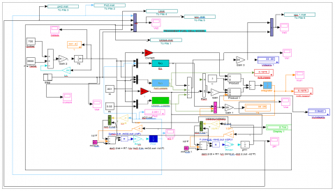
The prediction of an 18W fuel cell system using BP networks is studied. The system's stack voltage can be predicted by using two input variables, namely, hydrogen pressure and current. The other input variables include the system temperature, oxygen flow rate, hydrogen composition, and pressure. The training algorithm's accuracy is quite satisfactory. The system's stack is practically built. During tests, the various input and output parameters of the fuel cells are observed. The simulation model for the 18W fuel cell system is developed based on the input parameters. It then generates a simulation model that shows the system's performance. A good input parameter is fuel pressure, as it can help validate the model's performance. When the fuel cell's efficiency and voltage are varied, the output parameters of the fuel cell-like system are affected. The simulation diagram of a transient dynamic model of the fuel cell considering the pressure, temperature, and load variations is presented in Figure 5.
Figure 6. Transient a model under sudden change in load current
The varying pressures also affect the system’s current density. The simulation results indicated that BP networks could predict the system's stack voltage using only two input parameters.
Figure 7. Transient model voltage and current effects
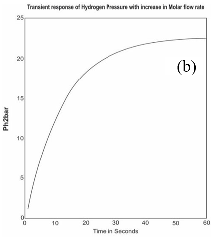
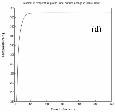
The voltage and current changes under the transient operation of a fuel cell are shown in Figures 6 and 7. The variation in the anode and cathode channels is also shown in Figure 8 and Figure 9. The transient response of temperature and voltage of the stack under a sudden change in load is shown in Figure 10. In addition, Figure 11 (a) represents the transients under sudden load change with an increase in molar flow rate, 11(b) represents the increase in voltage under transient operations, 11(c) represents the variations in the temperature and 11(d) shows the variations in the reactant pressures.
Figure 8. Anode and cathode channel temperature variations
Figure 9. Anode and cathode channel pressure variations
Figure 10. Transient response of temperature and voltage of the stack under a sudden change in load
Figure 11. Transients under sudden load change with an increase in molar flow rate; Notice the increase in voltage, temperature, and reactant pressures
5.1 Model validation with benchmarked studies
The dynamic model of a proton exchange membrane fuel cell was verified and validated by means of experiments. The authors focused on capturing transients in the cell voltage only. The model proposed by the authors requires at least 22 experimentally identified parameters. In order to minimize the complexity of the model, the authors suggested that the simplified versions be derived. The results of the study show that the model can be modeled using simple mathematical equations. The two models are then compared with the results of the experiments. The model shows the dynamic response of the cell to various parametric values such as temperature, capacitance, and mass flow rate.
The dynamic model is composed of all the subsystem level models that are independent of each other. The modifications and investigations of the dynamic model are performed to account for the various components of the model, such as the water content and temperature variations.
The parameters that are used to determine the effect of membrane humidity on fuel cell voltage are derived from the literature. An example of this effect is the polarization curve of the membrane water content. The results of the study are then compared with those obtained in the literature. The temperature variation in the system is then assumed to be constant. The concentration loss caused by the transient profile variations in the anode and cathode pressure can affect the performance of the stack. The polarization curve reflecting the variation in membrane water content is shown in Figure 12.
Figure 12. Polarization curves reflecting the variation in membrane water content
Different system models and their auxiliary components of the Transient model was represented in the Table 3.
Table 3. Transient model systems with auxiliary components
|
S. No |
Sub System |
Components |
|
1 |
Electrochemical |
Equilibrium Potential |
|
2 |
Electrochemical |
Activation over-voltage equation |
|
3 |
Electrochemical |
Ohmic overvoltage equation |
|
4 |
Capacitance |
Charge double-layer capacitance equation |
|
5 |
Anode Inlet |
Thermodynamic Relations |
|
6 |
Membrane Hydration |
Membrane water content equations |
| 7 | Manifold | Manifold Dynamic Equations |
In addition, the transients can vary from 0 to 7 seconds. They can also be caused by a complex electrode phenomenon that occurs in fuel cells.
Figure 13. Without capacitance model variations
The reaction depends on the charge entities of the protons and electrons on the surface of the membrane and the electrode. The voltage loss at the interface between the membrane and the electrode is caused by the activation voltage loss. The presence of a platinum catalyst on the electrodes increases the likelihood of a successful reaction. Figure 13 presents the variation of voltage without capacitance variations.
When a large current is flowing, the charge builds up at the interface, which can then lead to a small increase in the activation loss. The resistance of its membrane and electrodes respectively represents the activation resistance and the double- layer capacitance of a fuel cell.
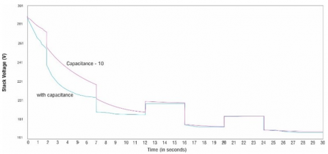
Figure 14. With capacitance model variations
This model is designed to simulate a complex reaction in a fuel cell. It is important to note that the circuit used in this model is not perfect for every fuel cell. The predictions made using this model are extremely accurate. The model provides a good understanding of the dynamic performance of a fuel cell. However, it is also suggested that a capacitance model be used to get a better understanding of the transient behavior of a fuel cell.
The charge double-layer capacitance of a fuel cell is measured using a current interrupt method. A fuel cell's transient profile can be analyzed by evaluating its characteristics without a double-charge capacitor. The graph shows that the initial jump in the stack voltage is caused by the rise in the cathode pressure. The activation overvoltage in the model could cause this phenomenon.
The presence of a double charge capacitor might prevent this overshoot effect from happening. The properties of the stack, such as electrical permittivity and the surface area of the electrodes, can affect the dynamic response of a fuel cell. The variation of fuel cell voltage with capacitance variations is shown in Figure 14. Table 4 represents the parameters of the transient model with their auxiliary components. Also, table 5 describes the coefficients of the MEA model used in the proposed test method.
Table 4. Parameters of the transient model with auxiliary components
|
Symbol |
Variable |
Specification |
|
$\rho_{m, d r y}$ |
Membrane Dry Density |
0.003 Kg/cm3 |
|
$M_{m, d r y}$ |
Membrane Dry Equivalent Weight |
1.1 Kg/mol |
|
$t_m$ |
Membrane Thickness |
0.1365 cm |
|
$J_c$ |
Compressor and Motor Inertia |
5 × 10⁻⁵ Kg. m2 |
|
$V_{a n}$ |
Anode Volume |
0.005 m3 |
|
$V_{c a}$ |
Cathode Volume |
0.01 m3 |
|
$V_{i m}$ |
Inlet Manifold Volume |
0.02 m3 |
|
$V_{\text {om }}$ |
Outlet Manifold Volume |
0.005 m3 |
|
$C_{D, o m}$ |
Outlet Manifold Throttle Discharge Coefficient |
0.0124 |
|
$A_{T, \mathrm{om}}$ |
Outlet Manifold Throttle Area |
0.002 m2 |
|
$k_{\text {im,out }}$ |
Inlet Manifold Outlet Orifice Constant |
0.3629 × 10⁻⁵ Kg/s. Pa |
|
$k_{\text {ca,out }}$ |
Cathode Outlet Orifice Constant |
0.2177 × 10⁻⁵ Kg/s. Pa |
|
$P_{a t m}$ |
Atmospheric Pressure |
101.325 k.Pa |
|
$T_{\text {atm }}$ |
Atmospheric Temperature |
298.15 K |
|
$\gamma$ |
The ratio of Specific Heat in Air |
1.4 |
|
$\rho_a$ |
Density of Air |
1.23 Kg/m3 |
|
$R_a$ |
Universal Gas Constant |
8.3145 J/(mol.K) |
|
$R_{O_2}$ |
Air Gas Constant |
286.9 J/(kg.K) |
|
$R_{N_2}$ |
Oxygen Gas Constant |
259.8 J/(kg.K) |
|
$R_{H_2}$ |
Vapor Gas Constant |
461.5 J/(kg.K) |
|
$M_{\mathrm{O}_2}$ |
Oxygen Molar Mass |
32E-3 Kg/mol |
|
$M_{N_2}$ |
Nitrogen Molar Mass |
28E-3 Kg/mol |
|
$M_v$ |
Vapor Molar Mass |
18.02E-3 Kg/mol |
|
$M_{H_2}$ |
Hydrogen Molar Mass |
2.016E-3 Kg/mol |
Table 5. Coefficients of MEA model
|
Symbol |
Value |
|
$\xi_1$ |
0.581 |
|
$\xi_2$ |
0.025365 |
|
$\xi_3$ |
1.044 × 10⁻⁴ |
|
$\xi_4$ |
-1.0028 × 10⁻³ |
|
$\xi_5$ |
-0.133 |
|
$\xi_6$ |
4.103 × 10⁻⁴ |
|
$\xi_7$ |
7.9584 × 10⁻⁴ |
This paper presents an AI-based model that can predict the operating temperature of a PEMFC. The model is trained offline using experimental data. The proposed model has a tracking error of less than 0.5%. It is tested under different conditions and the operating temperature of the neural network is determined using the experimental data. The results conclude that the proposed approach gives the best performance of the PEM fuel cell under different transient operating conditions model parameter variations.
[1] R. F. Mann, J. C. Amphlett, M. A. Hooper, H. M. Jensen, B. A. Peppley, and P. R. Roberge, "Development and application of a generalized steady-state electrochemical model for a PEM fuel cell," Journal of Power Sources, vol. 86, pp. 173-180, 2000, https://doi.org/10.1016/S0378-7753(99)00484-X.
[2] M. Ceraolo, C. Miulli, and A. Pozio, "Modelling static and dynamic behavior of proton exchange membrane fuel cells on the basis of electrochemical description," Journal of power sources, vol. 113, pp. 131-144, 2003, https://doi.org/10.1016/S0378-7753(02)00565-7.
[3] J. M. Correa, F. A. Farret, L. N. Canha and M. G. Simoes, "An electrochemical-based fuel-cell model suitable for electrical engineering automation approach," in IEEE Transactions on Industrial Electronics, vol. 51, no. 5, pp. 1103-1112, Oct. 2004, doi: 10.1109/TIE.2004.834972.
[4] M. Karthik and K. Gomathi, "Dynamic neural network based parametric modeling of PEM fuel cell system for electric vehicle applications," International Conference on Advances in Electrical Engineering (ICAEE), 2014, pp. 1-5, doi: 10.1109/ICAEE.2014.6838559.
[5] B. Sathya prabakaran and S. Paul, "Modeling and simulation of PEM fuel cell based power supply and its control," IET Chennai 3rd International on Sustainable Energy and Intelligent Systems (SEISCON 2012), 2012, pp. 1-6, doi: 10.1049/cp.2012.2231.
[6] M. Wöhr, K. Bolwin, W. Schnurnberger, M. Fischer, W. Neubrand, and G. Eigenberger, "Dynamic modelling and simulation of a polymer membrane fuel cell including mass transport limitation," International Journal of Hydrogen Energy, vol. 23, pp. 213-218, 1998, https://doi.org/10.1016/S0360-3199(97)00043-8
[7] J. Haubrock, G. Heideck and Z. Styczynski, "Dynamic Investigation on Proton Exchange Membrane Fuel Cell Systems," 2007 IEEE Power Engineering Society General Meeting, 2007, pp. 1-6, doi: 10.1109/PES.2007.385869.
[8] W. Friede, S. Rael and B. Davit, "Mathematical model and characterization of the transient behavior of a PEM fuel cell," in IEEE Transactions on Power Electronics, vol. 19, no. 5, pp. 1234-1241, Sept. 2004, doi: 10.1109/TPEL.2004.833449.
[9] Xin Kong, A. M. Khambadkone and Soy Kee Thum, "A hybrid model with combined steady-state and dynamic characteristics of PEMFC fuel cell stack," Fourtieth IAS Annual Meeting. Conference Record of the 2005 Industry Applications Conference, 2005, pp. 1618-1625 Vol. 3, doi: 10.1109/IAS.2005.1518663.
[10] F. da Costa Lopes, E. H. Watanabe and L. G. B. Rolim, "A Control-Oriented Model of a PEM Fuel Cell Stack Based on NARX and NOE Neural Networks," in IEEE Transactions on Industrial Electronics, vol. 62, no. 8, pp. 5155-5163, Aug. 2015, doi: 10.1109/TIE.2015.2412519.
[11] X. Guo and X. Yan, "Optimization Analysis of Hydrogen Fuel Cell Hybrid Power Based on Neural Network and Sensor Networks," 2021 5th International Conference on Intelligent Computing and Control Systems (ICICCS), 2021, pp. 172-175, doi: 10.1109/ICICCS51141.2021.9432118.
[12] W. Y. Lee, G. Park, T. H. Yang, Y. G. Yoon, and C. S. Kim, "Empirical modelling of polymer electrolyte membrane fuel cell performance using artificial neural networks," International Journal of Hydrogen Energy, vol. 29, pp. 961-966, 2004, doi:10.1016/j.ijhydene.2003.01.002
[13] S. JemeÏJemei, D. Hissel, M. PÉraPera and J. M. Kauffmann, "A New Modeling Approach of Embedded Fuel-Cell Power Generators Based on Artificial Neural Network," in IEEE Transactions on Industrial Electronics, vol. 55, no. 1, pp. 437-447, Jan. 2008, doi: 10.1109/TIE.2007.896480.
[14] A. U. Chávez, Ramírez, R., Muñoz Guerrero, S. Duron Torres, M. Ferraro, G. Brunaccini, F. Sergi, et al., "High power fuel cell simulator based on artificial neural network," International Journal of Hydrogen Energy, vol. 35, pp. 12125-12133, 2010, https://doi.org/10.1016/j.ijhydene.2009.09.071
[15] B. Blunier, M. G. Simões and A. Miraoui, "PEM Fuel Cell Stack Modeling for Real-Time Emulation in Hardware-in-the-Loop Applications," in IEEE Transactions on Energy Conversion, vol. 26, no. 1, pp. 184-194, March 2011, doi: 10.1109/TEC.2010.2053543.
[16] S. Elanayar V.T. and Y. C. Shin, "Radial basis function neural network for approximation and estimation of nonlinear stochastic dynamic systems," in IEEE Transactions on Neural Networks, vol. 5, no. 4, pp. 594- 603, July 1994, doi: 10.1109/72.298229.
[17] Wen-Jin Gu, Jun-Wei Lei and Yin-Hua Lei, "Single input RBF neural robust controller design for a class of nonlinear system with linear input unmodeled dynamics and unknown control function matrices," 2005 International Conference on Machine Learning and Cybernetics, 2005, pp. 4662-4666 Vol. 8, doi: 10.1109/ICMLC.2005.1527761.
[18] K. L. Priddy and P. E. Keller, Artificial neural networks: an introduction vol. 68: SPIE Press, 2005, https://doi.org/10.1117/3.633187.
[19] S. Ou and L. E. Achenie, "A hybrid neural network model for PEM fuel cells," Journal of Power Sources, vol. 140, pp. 319-330, 2005, https://doi.org/10.1016/j.jpowsour.2004.08.047.
[20] R. Sathya and A. Abraham, "Comparison of supervised and unsupervised learning algorithms for pattern classification," Int J Adv Res Artificial Intell, vol. 2, pp.34-38, 2013, doi:10.14569/IJARAI.2013.020206
[21] Bhoopal, N., Rao, D.S.M., Sireesha, N.V., Kasireddy, I., Gatla, R.K., Kumar, D.G. (2022). Modelling and performance evaluation of 18w PEM fuel cell considering H2 pressure variations. Journal of New Materials for Electrochemical Systems, Vol. 25, No. 1, pp. 1-6. https://doi.org/10.14447/jnmes.v25i1.a01.