Li Fu* | Xiuwei Fu | Ping Yang
© 2021 IIETA. This article is published by IIETA and is licensed under the CC BY 4.0 license (http://creativecommons.org/licenses/by/4.0/).
OPEN ACCESS
The power generation subsystem represents one of the principal components of a space system and is usually assembled from solar arrays and PPT topology. This paper aims to design and implement an algorithm to continuously extract the maximum power from the solar cells and deliver it to the consumer with minimum loss. In this regard, a brief introduction to the various parts of the power generation subsystem is provided and through accurate modeling of the solar cell and exploring the contributing factors to its power generation (including temperature, radiation, and space radiation), the algorithm is proposed based on the impedance matching concept. Simulation studies using MATLAB software have estimated an approximate 0.25065W per square centimeter power extraction and delivery to the customer. Our results suggest that the proposed approach can reduce steady-state losses while ensuring accuracy.
solar cell, maximum power point tracking, impedance matching concept, solar radiation, DC/DC converter
The rising concerns regarding fossil fuel depletion and environmental pollution worldwide have increasingly sparked the exploitation of renewable energies, in particular, solar cells and photovoltaic (PV) phenomenon. In recent years, PV technology has received a lot of attention due to its environmental and economic benefits. In photovoltaic power generation system, due to the high cost of PV modules and their low conversion efficiency, the exploitation of available power must be optimized efficiently. Optimizing the performance of PV generators using power conversion systems is referred to as MPPT tracking [1]. Using the voltage / current characteristics of PV modules, the deformation capability is limited [2].
With the ever-increasing advances in satellite and spacecraft technology and the surge in the number of space missions, the solar cells have emerged as an inevitable source of power generation. Many satellites and spacecrafts have no option to supply their required electrical energy other than utilizing the solar cells [3].
The power supply systems are divided into two general categories: 1- Power control and distribution system and 2- Power generation sources. The power control and distribution systems include direct energy transfer (DET) and peak power tracker (PPT) systems. Power regulation in DETs is carried out by the dissipation of excess power through parallel voltage regulators leading to a high loss, while PPT offers a loss-free power regulation via operating point control of solar arrays [4]. The satellite power generation sources are dependent on many factors, including the mission duration and the amount of energy needed. For missions longer than one year, three different power generation systems can be described as follows: (i) static power generation systems that convert the thermal energy of the sunlight or nuclear sources to the electrical power. An example of such a system is radioisotope thermonuclear generator (RTG) used for manned and far-sun spacecraft [3]; (ii) dynamic power generation systems that utilize the thermodynamic cycle to produce electrical power in remote space missions requiring high power consumption. The concentrated solar energy, radioisotopes, and nuclear fusion can serve as the inputs to these systems [5]; and (iii) PV systems are the most common energy generation source in space systems in which the solar cells play a significant role.
Maximum power point tracking (MPPT) is an essential component of energy production in a photovoltaic (PV) system. Numerous articles have examined different methods of MPPT control. [2] In the real world, MPPT testing is not easy, and its preparation is time consuming. Due to the characteristics of PV, which is very high voltage and low current so that the inverter cannot work. On the other hand, there are special requirements for linearity in terms of MPPT test [6]. MPPT usually uses a DC-DC converter to adapt the impedance for extracting the maximum possible power from the PV plate by continuously adjusting of the control signal cycle. Over the past few decades, countless MPPT control algorithms have been proposed. These MPPT methods differ in many aspects, including the sensors used, hardware performance, cost and etc. [7]
This article deals with the study of the PV-based power generation systems in satellites. Accordingly, in the second section, the structure of photovoltaic cells is studied. In the third section, a proposed algorithm for MPPT is presented, and in the fourth and fifth sections, conclusions and future suggestions are given, respectively.
PV phenomenon represents a mechanism by which the solar radiation energy is directly converted into electrical energy. This energy that needs no intermediary process is called the PV effect and is defined as the electrical potential produced as a result of light incident on two dissimilar semiconductors [8].
Edmond Becquerel was the first to notice this effect in 1839. However, it wasn't until 1958 that Hans Ziegler (the father of solar power) designed the first satellite based on this concept [9, 10]. Other than the solar cell, a PV system consists of a DC/DC converter, battery, and maximum power point tracking system [11] that will be briefly introduced in the following sections.
2.1 Solar cells
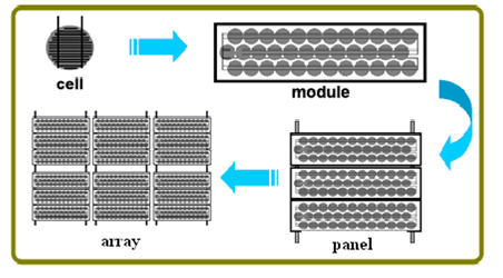
As seen from the Figure 1, the solar cells connected in series form a string, and several strings arranged alongside each other create the solar module. The interconnected modules constitute a solar panel, and an assembly of these panels is referred to as a solar array [12].
Figure 1. Solar cells are the basis of PV systems. These cells, alongside each other, form the modules. The modules create the panels and then arrays (reprinted from [12] with permission)
The primary constituent material of the solar cells -which convert the sunlight energy to the electrical power- is a thin layer of semiconductor elements (the fourth layer in the periodic table). A PV cell is made by doping the main semiconducting material with N-type (elements in the fifth layer such as phosphorus) or P-type (elements in the third layer such as boron) impurities. Briefly, the electrons in the semiconductor are polarized by absorbing the solar radiation (negative electrons in N-type impurity and positive electrons in P-type impurity). This establishes a potential difference between the two electrodes and photon current flows [13]. The physics is much similar to the performance of a diode [9]. Indeed, only a portion of photon energy contributes to power generation, and a great portion will dissipate as heat and increase the temperature of the solar cell. The solar cells are classified into three different generations. The first-generation cells are mostly made of silicon (Si) and Gallium Arsenide (GaAs), that each material presents its benefits and limitations [14]. The second-generation cells are called thin-film solar cells [15]. The members of the third generation are nanostructure cells that are mainly comprised of dye-sensitized solar cells (DSSCs), and their objective is to achieve high efficiency with minimum cost [14]. These modules are designed in either sandwich-like or monolithic forms. In sandwich-like structure (W and Z modules), the opposite electrodes are placed on either cell surfaces, while in the monolithic module, both electrodes are placed on one surface. For further detail on the various types of these modules, the reader can refer to [14, 15, 17, 18-21].
The contributing factors to solar characteristics reside in four major categories of the radiation angle and intensity, shadowing, temperature, and space radiation effects (that means the four general groups of neutron environment, radiation environment, plasma environment, and other environments such as micrometeorites). These factors are elaborated in detail in [8, 9, 22, 19, 23-29].
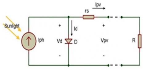
Numerous models have been proposed for solar cells and are studied extensively in [5, 6, 11, 15, 23, 30-39]. As shown in Figure 2, the solar cell model consists of four sections: (1) the current source resulting from the incident light that models the electrons and holes induced by light absorption in the semiconductor; (2) the parallel diode to the source that models the diffusive current or diffusion; (3) the parallel resistance to the diode that models a portion of loss carriers produced by crystal surfaces or improper connections; and (4) the series resistance to the model that is a result of the path where the light-generated electrons are forced to pass.
Figure 2. The equivalent electrical circuit of a solar cell (reprinted from [11] with permission)
According to Figure 2, the relationship between the output voltage and current of the solar cells is described as:
$I={{I}_{P}}-{{I}_{D}}-\text{ }\!\!~\!\!\text{ }\frac{V+I{{R}_{s}}}{{{R}_{sh}}}$ (1)
In order to have a more accurate description, by placing the elements of equation (1) as follows, we can reach the general equation (2):
${{I}_{P}}={{I}_{{{P}_{o}}}}\left( \frac{P}{{{P}_{o}}} \right)\left( 1+{{K}_{o}}\left( T-{{T}_{o}} \right) \right)-Clog\left( 1+\phi /{{\phi }_{x}} \right)$ (1-1)
${{I}_{{{P}_{o}}}}=\Re A{{P}_{o}}$ (1-2)
$J=\left( \frac{q{{D}_{P}}}{{{L}_{P}}}{{P}_{{{n}_{o}}}}+\frac{q{{D}_{n}}}{{{L}_{n}}}{{n}_{{{P}_{o}}}} \right)\left( {{e}^{\frac{q\left( V+I{{R}_{S}} \right)}{KT}}}-1 \right)+\frac{q{{n}_{i}}W}{2{{\tau }_{e}}}\left( {{e}^{\frac{q\left( V+I{{R}_{S}} \right)}{KT}}}-1 \right)$ (1-3)
${{n}_{{{P}_{o}}}}=\frac{n_{i}^{2}}{{{N}_{A}}},~{{P}_{{{n}_{o}}}}=n_{i}^{2}/{{N}_{D}}$ (1-4)
${{R}_{sh}}={{R}_{s{{h}_{0}}}}\text{exp}\left( {{K}_{1}}\left( T-{{T}_{0}} \right) \right)$ (1-5)
${{R}_{s}}={{R}_{{{s}_{0}}}}\left[ 1+{{K}_{2}}\left( T-{{T}_{0}} \right) \right]$ (1-6)
Substituting the corresponding elements from [8, 23, 31-35] into the equation (1) yields the following general relation:
$I=\text{ }\!\!~\!\!\text{ }{{I}_{{{P}_{O}}}}\left( \frac{P}{{{P}_{O}}} \right)\left( 1+K\left( T-{{T}_{0}} \right) \right)-Clog\left( 1+\phi /{{\phi }_{x}} \right)$
$-A\left( \frac{q{{D}_{P}}}{{{L}_{P}}}{{P}_{{{n}_{O}}}}+\frac{q{{D}_{n}}}{{{L}_{n}}}{{n}_{{{P}_{o}}}} \right)\left( {{e}^{q\left( V+I{{R}_{s}} \right)/KT}}-1 \right)+A\frac{q{{n}_{i}}W}{2{{\tau }_{e}}}\left( {{e}^{q\left( V+I{{R}_{s}} \right)/2KT}}-1 \right)-\frac{V+I{{R}_{s}}}{{{R}_{sh}}}$ (2)
The solar cell parameters used in relation (2) and their corresponding simulation values are provided in the Table 1.
Table 1. The numerical values of the parameters used in the simulation of solar cells [8]
|
Parameter |
Definition |
Numerical value |
|
I |
The solar cell output current |
[2.5 3.7] |
|
V |
The solar cell output voltage |
|
|
$I_{P_{o}}$ |
The initial photo-generated current |
$\mathfrak{R}$ AP0 |
|
P |
Sunlight radiation |
1000 |
|
P0 |
Initial sunlight radiation |
|
|
K |
Boltzmann's constant |
1.38×10⁻²³ |
|
T |
Solar cell temperature |
30 |
|
T0 |
Solar cell initial temperature |
28 |
|
C |
Radiation coefficient |
56.2 |
|
A |
Solar cell surface area |
1 cm2 |
|
q |
Electron charge |
1.6×10⁻¹⁹ |
|
Dp |
Hole diffusion coefficient |
12.5 |
|
Lp |
Hole diffusion length |
7.13×10¹⁴ |
|
$\boldsymbol{R}_{\boldsymbol{s}_{0}}$ |
Initial parallel resistance in the equivalent circuit |
0.008 |
|
$\boldsymbol{R}_{s h_{0}}$ |
Initial parallel resistance in the equivalent circuit |
5000 |
|
Ln |
Electron diffusion length |
7.13×10¹⁴ |
|
$\boldsymbol{n}_{\boldsymbol{p}_{\boldsymbol{o}}}$ |
Amount of majority carriers outside the depletion region |
$n_{P_{0}}=n_{i}^{2} / N_{A}$ |
|
Rs |
The series resistance of the equivalent circuit |
Rs0[1+k2(T-T0)] |
|
ni |
The concentration of intrinsic carrier |
1.5×10¹⁰ |
|
W |
The width of the depletion region |
0.25 |
|
$\boldsymbol{R}_{\boldsymbol{s h}}$ |
The parallel resistance of the equivalent circuit |
Rsho exp(K1(T-T0)) |
|
$\boldsymbol{\phi}$ |
Environmental radiation |
$\phi_{x}$ |
|
$\phi_{x}$ |
The amount of radiation needed for sensible variations in Ip |
|
|
$\boldsymbol{\tau}_{\boldsymbol{e}}$ |
The lifetime of minority carriers due to electrons radiation |
10-7 |
|
$\mathfrak{R}$ |
The solar cell response |
0.3 |
|
ND |
The concentration of donors in N-region |
5×10¹⁶ |
|
NA |
The concentration of acceptors in P-region |
1017 |
|
Dn |
Electron diffusion coefficient |
35 |
|
$\boldsymbol{P}_{\boldsymbol{n}_{\boldsymbol{o}}}$ |
The amount of minority carriers outside the depletion region |
$P_{n_{Q}}=n_{i}^{2} / N_{D}$ |
|
K1 |
Temperature constant of the equivalent circuit series resistance |
0.002 |
|
K2 |
Temperature constant of the equivalent circuit parallel resistance |
0.002 |
2.2 DC to DC converter
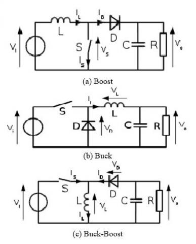
The switched-mode power supplies (SMPS) are used in both battery-using systems and solar cells owing to their high efficiency, low waste heat production, and voltage regulation capacity at different levels. They are classified into three main and highly applicable categories of voltage step-up (Boost (Figure 3-a)), voltage step-down (Buck (Figure 3-b)), and voltage step-down/step-up ((Buck-Boost (Figure 3-c)) converters. The main difference in these three Figures lies in the placement of the switch, inductor, and diode.
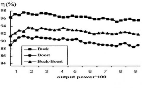
The major drawback associated with SMPSs is the incidence of noise and electromagnetic interference (EMI) during high-frequency switching [21]. A detailed review of various types of converters is presented in [7, 30, 40-47]. However, as shown in Figure 4, the voltage Buck converter efficiency is greater than its two other counterparts and is estimated at around 95% [21].
There is a straightforward relationship between the input and output impedance of the converter and its operation period, which is of great importance in dynamic impedance systems and also for the employment of the impedance matching. Given the fact that the power is constant, the current increases as the voltage reduces, which justifies the selection of these converters. When the switch is off, the current starts to increase, and with the voltage drop on the source, the output voltage reduces, and the inductor begins to store the magnetic energy. When the switch turned on, the source is disconnected from the circuit, and the inductor becomes responsible for the load energy supply. With suitable switching frequency (before the inductor is fully discharged), the voltage level always remains higher than zero [41]. In order to fulfill the converter stability criterion, the stored energy in each part at the beginning, and the end of the variation period should always be equal. Assuming that only the inductor is variable and its energy is proportional to the current variations, the relationship between the current in on/off states can be expressed in terms of the relation (8). By taking their sum equal to zero, the operation period reduces to the relation (9). From this and taking into account the ohm law, the operation period derives from equation (10). The recent relation suggests that the Buck converter will transfer the maximum power according to the impedance matching theory.
Figure 3. A simple schematic of converters
Figure 4. the efficiency of Buck, Boost, and Buck-Boost converters (reprinted from [48] with permission)
Note: This figure is based on the same output power in the horizontal axis for converters
$\begin{align} & \text{ }\!\!\Delta\!\!\text{ }{{\text{I}}_{{{\text{L}}_{\text{on}}}}}=\left( {{V}_{i}}-{{V}_{o}} \right)\frac{DT}{L} \\ & \text{ }\!\!\Delta\!\!\text{ }{{\text{I}}_{{{\text{L}}_{\text{off}}}}}=\left( -{{V}_{o}} \right)\frac{\left( 1-D \right)T}{L} \\\end{align}$ (4)
$\text{ }\!\!~\!\!\text{ }\!\!\Delta\!\!\text{ }{{I}_{{{L}_{on}}}}+\text{ }\!\!\Delta\!\!\text{ }{{I}_{{{L}_{off}}}}=0$ (5)
$D=\frac{{{V}_{i}}}{{{V}_{o}}}$ (6)
2.3 Battery
The batteries offer two essential benefits in the satellite power systems:
i) Storing the surplus power to compensate for power loss during the developed power variation
ii) For voltage supply and settlement in the circuit [49]
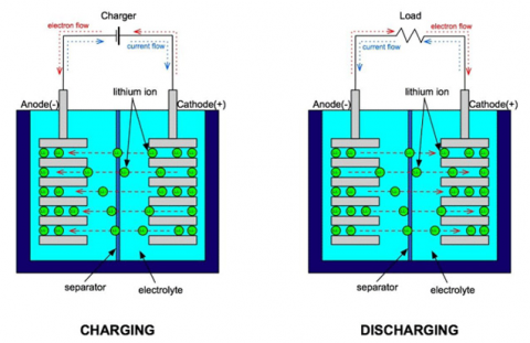
During the shadowing period, the solar cell lacks any power, and batteries provide a possible means to supply the required energy. According to Figure 5, two distinct chemical reactions take place in a battery to generate electrical energy. First, oxidation occurs between the anode (negative electrode) and electrolyte, and the positively charged ions and free electrons are transferred to the electrolyte. In the reduction process, the free electrons migrate toward the cathode (positive electrode), and as a result, the positive ions and the electrons recombine together [50]. The batteries are classified based on their electrode material and electrolyte solution. With regard to the intended application, three general categories of lithium [13, 51-56], Nickle [11], and nano-phosphate [30, 57-58] batteries can be mentioned.
Figure 5. The charge and discharge processes in lithium batteries (reprinted from [51] with permission)
The lithium-ion battery is constructed from lithium cobalt oxide as the cathode, carbon as the anode and lithium salt in an organic solvent as the electrolyte. During the charging process, the metal lithium present in cathode converts to lithium-ion, and the lithium ions in the electrolyte are stored between the carbon layers (graphite). The most significant features of such batteries include their lack of memory effect, extremely low self-discharge rate, high voltage capacity, fast ion transfer rate, high power delivery, light weight, and around 1000 cycles depth of discharge (DOD) [41]. A key limitation of these batteries is the infeasibility of using water as an electrolyte due to the high reactivity of lithium. The use of organic solvents as electrolytes increases the danger of inflammation during charge and discharge processes, and thus complying the safety design requirements is a necessity for their application, which in turn raises the final cost of the project [51, 52].
Of various kinds of batteries used in the satellite supply systems, the nano-phosphate batteries can be pointed out where the reduction rate and output power rise with the cathode surface area. The characteristics of the nano-phosphate batteries are studied in detail in [30, 57-58].
2.4 Maximum power point tracking (MPPT)
Numerous techniques exist to find the maximum power point, and there are different classifications for them. One classification includes a basic algorithm like Perturb and Observe (P&O), while the other consists of the methods based on a certain model of the solar cell; the third classification focuses on the existing relationship between the working point and solar cell parameters, and the fourth one is the smart control algorithms [3].
Other classifications are introduced for maximum power point tracking in [3]. In [59], all methods fall into two general groups of dynamic and non-dynamic algorithms. In [3, 38], the specific MPPT approaches are elaborated in detail. Generally, no method can be regarded as best practice. Criteria such as construction cost, tracking speed, the accuracy of the determined point, simplicity of implementation, generality, and flexibility can be investigated among others [3].
For instance, the P&O method has a long history and, to simply put, it explores the system behavior by applying an initial disturbance. This method can be integrated with other techniques for optimization, as in [60, 8, 24, 61, 62-63, 64-66]. In [8], the maximum power point tracking is performed based on a specified time interval and variation of the operation period with time while averaging the input data (around 0.1015 W power per square centimeter). In [60], the ratio of open-circuit voltage to short-circuit current is employed for optimization of P&O approach (around 0.1040 W power per square centimeter)
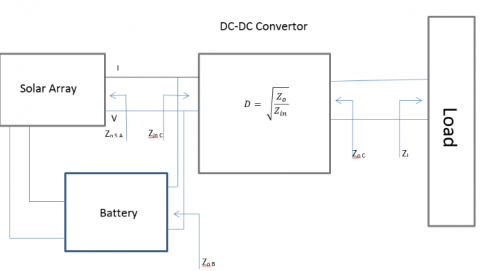
The main objective of the proposed algorithm is to design a simple system with the lowest complexity and highest flexibility in the placement of its various parts. We believe that the extraction of the maximum power from the solar cell is not the end of the road, and the algorithm should continue to power transfer and its delivery to the consumer (according to the impedance matching concept). Also, the designed algorithm incorporates the shadowing period. The block diagram of the scheme is depicted in Figure 6.
Figure 6. The overall block diagram of the proposed algorithm
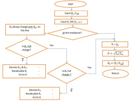
The presented algorithm as shown in Figure 7 such as flowchart, unlike the existing ones, starts from the end that is from the consumption load. This is because the algorithm is expected to continue until the load transfer and delivery stage.
The impedance matching algorithm for MPPT can be described in the following steps:
Step I: Initially, the load impedance value is calculated
Step II: It should be justified whether the solar cell is under shadow or sunshine.
Step III: If it is shadowed, the matching action is performed with battery cells; otherwise, it is performed with solar cells.
Step IV: Providing that the load impedance is equal to the converter's output impedance and from the operation period relation, we can achieve the converter input impedance according to Figure 6.
Step V: The converter's input impedance is the output impedance of the solar or battery cells. In this step, taking into account the optimal value of resistance obtained for each cell in MPPT, we can achieve the required number of cells connected to the circuit so that transfer the maximum power based on the impedance matching concept.
The flowchart of the proposed algorithm is demonstrated in Figure 7.
Figure 7. The flowchart related to the impedance matching algorithm for MPPT
The duty cycle of the converter (D) and the output resistance of a solar cell unit (ZSA) and the load resistance or the relationship between voltage and load current are shown in Figures 6 and 7. According to these inputs and the algorithm presented above, it is possible to store energy in the battery and use the correct number of solar cell units as input (or use the correct number of battery units when there is no radiation) to implement the concept of impedance matching. This algorithm first accurately calculates the load impedance. It then implements the concept of matching impedance with solar cells or battery cells, respectively, by determining whether it is in radiation or shading conditions. In the simulation process, a variable can be used to enter the required number of cells into the circuit according to the optimal value of resistance obtained for each cell at its maximum power point according to the impedance matching, then the maximum power obtained is transferred to the load.
(a)
(b)
(c)
(d)
(e)
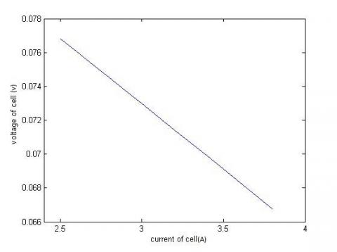
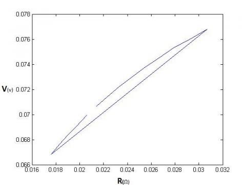
Figure 8. (a) voltage-current, (b) power-voltage, (c) 3D resistance-power-voltage, (d) voltage-resistance and (e) power-resistance plots
Note: In these figures, power in watts, voltage in volts, resistance in ohms and current in amps are listed.
For the simulation, we utilize the relation (2) and Table 1 in which all the space conditions are presented. For a 0.26 mH inductance, a 42.38 µF capacitor, a 16.48 Ω resistance, and a switching frequency of 50 kHz, we will have a Buck converter with 84% operation period. Since there are two unknown terms in equation (2), we apply the current data placement to solve the equation. If we take the current range as [2.5 3.8] (the minimum and maximum current value in a solar cell following [2, 6]), by solving the equation in MATLAB software, we can draw the voltage-current, power-voltage, voltage-resistance, and power-resistance plots and also a 3D plot of resistance-power-voltage as shown in Figure 8.
According to these plots and the relation (2), for a 3.75 A current and 0.06684 V voltage, the optimal ohm resistance of a 1 cm2 solar cell is obtained as 0.017824 Ω. This suggests that we can achieve a power equal to 0.25065 W using our proposed algorithm. The obtained power is about two-fold of the values reported by similar algorithms.
In the case that the cells are connected in series, according to Figure 7, a counter like Ns can yield the number of series cells needed for matching the output impedance with the source internal resistance based on the impedance matching concept.
The utilization of three separate battery packs (consisting of multiple cells) is also proposed. One battery pack always at its final 50 percent charge level is used as a backup while the other two packs meet the system demands with the battery charge always above 20% of its final value. Therefore, the lower need for regular charging of the batteries enhances their lifetimes. Each battery pack can include several smaller cells. They are connected to the circuit, as mentioned above, to apply the impedance matching concept and the proposed algorithm.
This paper presents a novel approach for maximum power point tracking based on the impedance matching concept. The study involves the simulation of the contributing factors to solar cell performance according to relation (2), the measurement of the output impedance of power generation circuit per second and taking it equal to the source impedance (which can comprise of solar arrays or batteries). These efforts lead to tracing the maximum power derived from the source and its delivery to the consumer. One of the significant features of the proposed algorithm is the extraction of the maximum power and transferring it to the consumer. Based on this algorithm, the maximum power per square centimeter is obtained as 0.2568 W which is about two-fold of the compared similar cases.
Future studies should involve the design and implementation of this algorithm in the form of a PV source system. Microcontrollers or FPGA can be used for this implementation. The next issue is the utilization of current probability density rather than data placement for its value in the equation. By doing so, one can benefit from optimization algorithms such as Imperialist Competitive and neural-fuzzy. As the proposed algorithm without optimization yields an approximately two-fold power, finding a better solution by optimization might be feasible. Another issue that should be pointed out is the design of a sub-algorithm to achieve the optimal configuration rather than a series configuration. Ultimately, to avoid the losses and also reducing the volume, design of an integrated circuit consisting of the entire MPPT control sections and also the considered converter may be warranted. Closer attention to the space considerations, exploring the battery charge control system, and smart control of the reduction route are also of significance.
[1] Berrezzek, F., Khelil, K., Bouadjila, T. (2020). Efficient MPPT scheme for a photovoltaic generator using neural network. In 2020 1st International Conference on Communications, Control Systems and Signal Processing (CCSSP), 503-507. https://doi.org/10.1109/CCSSP49278.2020.9151551
[2] Priyadarshi, N., Padmanaban, S., Holm-Nielsen, J.B., Blaabjerg, F., Bhaskar, M.S. (2019). An experimental estimation of hybrid ANFIS–PSO-based MPPT for PV grid integration under fluctuating sun irradiance. IEEE Systems Journal, 14(1): 1218-1229. https://doi.org/10.1109/JSYST.2019.2949083
[3] Salvador, A. (2005). Energy: A historical perspective and 21st century forecast. American Association of Petroleum Geologists. ISBN Number: 978-1-58861-504-6
[4] Kim, S.J., Cho, B.H. (1990). Analysis of spacecraft battery charger systems. In Proceedings of 25th Intersociety Energy Conversion Engineering Conference (IECEC), 365-372. https://doi.org/10.1109/IECEC.1990.716917
[5] Salas, V., Olias, E., Barrado, A., Lazaro, A. (2006). Review of the maximum power point tracking algorithms for stand-alone photovoltaic systems. Solar Energy Materials and Solar Cells, 90(11): 1555-1578. https://doi.org/10.1016/j.solmat.2005.10.023
[6] Huang, W., Shu, M., Li, T., Sun, Y., Ma, L. (2020). MPPT test based on hardware-in-the-loop simulation platform of photovoltaic systems. In 2020 IEEE 3rd International Conference on Electronics Technology (ICET), 463-466. https://doi.org/10.1109/ICET49382.2020.9119670
[7] Berrezzek, F., Khelil, K., Bouadjila, T. (2020). Efficient MPPT scheme for a photovoltaic generator using neural network. In 2020 1st International Conference on Communications, Control Systems and Signal Processing (CCSSP), 503-507. https://doi.org/10.1109/CCSSP49278.2020.9151551
[8] Subudhi, B., Pradhan, R. (2012). A comparative study on maximum power point tracking techniques for photovoltaic power systems. IEEE Transactions on Sustainable Energy, 4(1): 89-98. https://doi.org/10.1109/TSTE.2012.2202294
[9] Patel, M.R. (2005). Wind and solar power systems: Design, analysis, and operation. CRC Press.
[10] Holmes-Siedle, A., Adams, L. (1993). Handbook of radiation effects.
[11] Jiang, Z., Liu, S., Dougal, R.A. (2002). Virtual-prototyping satellite electrical power systems using the virtual test bed. In Proceedings IEEE SoutheastCon 2002 (Cat. No. 02CH37283), 113-120. https://doi.org/10.1109/SECON.2002.995569
[12] Vaughan, J. (2019). Solar energy generation in desert climates. Available at SSRN 3609856. Vaughan, Jim, Solar Energy Generation in Desert Climates (June 23, 2019). http://dx.doi.org/10.2139/ssrn.3609856
[13] Raman, P., Murali, J., Sakthivadivel, D., Vigneswaran, V.S. (2012). Opportunities and challenges in setting up solar photo voltaic based micro grids for electrification in rural areas of India. Renewable and Sustainable Energy Reviews, 16(5): 3320-3325. https://doi.org/10.1016/j.rser.2012.02.065
[14] Zhang, C., Cvetanovic, S., Pearce, J.M. (2017). Fabricating ordered 2-D nano-structured arrays using nanosphere lithography. MethodsX, 4: 229-242. https://doi.org/10.1016/j.mex.2017.07.001
[15] Dahrul, M., Alatas, H. (2016). Preparation and optical properties study of CuO thin film as applied solar cell on LAPAN-IPB Satellite. Procedia Environmental Sciences, 33: 661-667. https://doi.org/10.1016/j.proenv.2016.03.121
[16] Harvey, T.J., Jones, P.A. (1994). U.S. Patent No. 5,298,085. Washington, DC: U.S. Patent and Trademark Office.
[17] Harvey, T.J., Jones, P.A. (1994). U.S. Patent No. 5,296,044. Washington, DC: U.S. Patent and Trademark Office.
[18] Gaddy, E.M. (1996). Cost performance of multi-junction, gallium arsenide, and silicon solar cells on spacecraft. In Conference Record of the Twenty Fifth IEEE Photovoltaic Specialists Conference-1996, pp. 293-296. https://doi.org/10.1109/PVSC.1996.564003
[19] Yoon, C.H., Vittal, R., Lee, J., Chae, W.S., Kim, K.J. (2008). Enhanced performance of a dye-sensitized solar cell with an electrodeposited-platinum counter electrode. Electrochimica Acta, 53(6): 2890-2896. https://doi.org/10.1016/j.electacta.2007.10.074
[20] Najam, A., Cleveland, C.J. (2005). Energy and sustainable development at global environmental summits: An evolving agenda. In The world summit on sustainable development, 113-134. https://doi.org/10.1007/1-4020-3653-1_5
[21] Massarrat, M. (2004). Iran’s energy policy: Current dilemmas and perspective for a sustainable energy policy. International Journal of Environmental Science & Technology, 1(3): 233-245. https://doi.org/10.1007/BF03325838
[22] Koomanoff, F.A. (1980). Satellite power system concept development and evaluation program. In sps.
[23] Anspaugh, B.E. (1996). GaAs solar cell radiation handbook.
[24] Hsiao, Y.T., Chen, C.H. (2002). Maximum power tracking for photovoltaic power system. In Conference Record of the 2002 IEEE Industry Applications Conference. 37th IAS Annual Meeting (Cat. No. 02CH37344), 1035-1040. https://doi.org/10.1109/IAS.2002.1042685
[25] Schimmerling, W. (2016). Genesis of the NASA space radiation laboratory. Life sciences in space research, 9: 2-11. https://doi.org/10.1016/j.lssr.2016.03.001
[26] Kieffer, P., Armbruster, P., Gerner, J.L., de Lande Long, M. (2004). European cooperation for space standardization (ECSS) space communication standards. ESASP, 570: 32.
[27] Tada, H.Y., Carter Jr, J.R., Anspaugh, B.E., Downing, R.G. (1982). Solar cell radiation handbook.
[28] Anspaugh, B.E., Downing, R.G. (1984). Radiation effects in silicon and gallium arsenide solar cells using isotropic and normally incident radiation.
[29] Anspaugh, B.E. (1989). Solar cell radiation handbook. Addendum, 1: 1982-1988.
[30] Skyttemyr, K.O. (2013). Design and implementation of the electrical power system for the CubeSTAR satellite. Master's thesis.
[31] Shekoofa, O., Taherbaneh, M. (2007). Modelling of silicon solar panel by MATLAB/Simulink and evaluating the importance of its parameters in a space application. In 2007 3rd International Conference on Recent Advances in Space Technologies, 719-724. https://doi.org/10.1109/RAST.2007.4284087
[32] Pongratananukul, N. (2005). Analysis and simulation tools for solar array power systems.
[33] Jiang, Z., Dougal, R.A., Liu, S. (2003). Application of VTB in design and testing of satellite electrical power systems. Journal of Power Sources, 122(1): 95-108. https://doi.org/10.1016/S0378-7753(03)00360-4
[34] Liu, S., Dougal, R.A. (2000). Solar Array Model.
[35] Sze, S.M. (2008). Semiconductor devices: Physics and technology. John Wiley & Sons.
[36] Skyttemyr, K.O. (2013). Design and implementation of the electrical power system for the CubeSTAR satellite, Master's thesis.
[37] Castaner, L., Silvestre, S. (2002). Modelling photovoltaic systems using PSpice. John Wiley and Sons.
[38] Esram, T., Chapman, P.L. (2007). Comparison of photovoltaic array maximum power point tracking techniques. IEEE Transactions on energy conversion, 22(2): 439-449. https://doi.org/10.1109/TEC.2006.874230
[39] Sahli, M., Correia, J.P.M., Ahzi, S., Touchal, S. (2018). Multi-physics modeling and simulation of heat and electrical yield generation in photovoltaics. Solar Energy Materials and Solar Cells, 180: 358-372. https://doi.org/10.1016/j.solmat.2017.07.039
[40] Benedict, R.R., Weiner, N. (1965). Industrial electronic circuits and applications. Prentice-Hall.
[41] Chiacchiarini, H., Mandolesi, P., Oliva, A. (1999). Nonlinear analog controller for a buck converter: Theory and experimental results. In ISIE'99. Proceedings of the IEEE International Symposium on Industrial Electronics (Cat. No. 99TH8465), 601-606. https://doi.org/10.1109/ISIE.1999.798680
[42] Floyd, T. L. (2007). Electronic Devices (Electron Flow Version). Prentice-Hall, Inc.
[43] Ott, H.W., Ott, H.W. (1988). Noise reduction techniques in electronic systems, 442. New York: Wiley.
[44] D'Amico, M.B., Oliva, A., Paolini, E., Guerin, N. (2006). Bifurcation control of a buck converter in discontinuous conduction mode. IFAC Proceedings Volumes, 39(8): 389-394. https://doi.org/10.3182/20060628-3-FR-3903.00069
[45] Nelson, C. (1986). Lt1070 design manual. Linear Technology Corporation, Application Note, 19.
[46] Oliva, A.R., Chiacchiarini, H.G., Bortolotto, G. (2005). Development of a state feedback controller for the synchronous buck converter.
[47] Chierchie, F., Paolini, E.E. (2009). Discrete-time modeling and control of a synchronous buck converter. In 2009 Argentine School of Micro-Nanoelectronics, Technology and Applications, 5-10.
[48] Masoum, M., Dehbonei, H. (1999). Design, construction and testing of a voltage-based maximum power point tracker (VMPPT) for small satellite power supply.
[49] Liedholm, E. (2010). Tracking the maximum power point of solar panels. A digital implementation using only voltage measurements.
[50] Wakihara, M. (2001). Recent developments in lithium ion batteries. Materials Science and Engineering: R: Reports, 33(4): 109-134. https://doi.org/10.1016/S0927-796X(01)00030-4
[51] Huang, S., Wen, Z., Yang, X., Gu, Z., Xu, X. (2005). Improvement of the high-rate discharge properties of LiCoO2 with the Ag additives. Journal of Power Sources, 148: 72-77. https://doi.org/10.1016/j.jpowsour.2005.02.002
[52] Kiehne, H.A. (2003). Battery technology handbook (Vol. 118). CRC Press.
[53] Zhang, S.S. (2006). A review on electrolyte additives for lithium-ion batteries. Journal of Power Sources, 162(2): 1379-1394. https://doi.org/10.1016/j.jpowsour.2006.07.074
[54] Peng, Z.S., Wan, C.R., Jiang, C.Y. (1998). Synthesis by sol–gel process and characterization of LiCoO2 cathode materials. Journal of Power Sources, 72(2): 215-220. https://doi.org/10.1016/S0378-7753(97)02689-X
[55] Wakihara, M. (2001). Recent developments in lithium ion batteries. Materials Science and Engineering: R: Reports, 33(4): 109-134. https://doi.org/10.1016/S0927-796X(01)00030-4
[56] Lu, C.H., Yeh, P.Y. (2001). Surfactant effects on the microstructure and electrochemical properties of emulsion-derived lithium cobalt oxide powders. Materials Science and Engineering: B, 84(3): 243-247. https://doi.org/10.1016/S0921-5107(01)00613-4
[57] Wang, J.P. (2013). Application of lithium-ion battery technology to the new energy vehicles. In Applied Mechanics and Materials, 273: 75-80. https://doi.org/10.4028/www.scientific.net/AMM.273.75
[58] Jeevarajan, J., Strangways, B., Nelson, T. (2009). Performance and safety evaluation of high-rate 18650 lithium ironphosphate cells. In NASA Battery Workshop.
[59] Brambilla, A., Gambarara, M., Torrente, G. (2002). Perturb and observe digital maximum power point tracker for satellite applications. In Space Power, 502: 263.
[60] Patil, M., Deshpande, A. (2015). Design and simulation of perturb and observe maximum power point tracking using matlab/simulink. In 2015 International Conference on Industrial Instrumentation and Control (ICIC), pp. 1345-1349. https://doi.org/10.1109/IIC.2015.7150957
[61] Pan, C.T., Chen, J.Y., Chu, C.P., Huang, Y.S. (1999). A fast maximum power point tracker for photovoltaic power systems. In IECON'99. Conference Proceedings. 25th Annual Conference of the IEEE Industrial Electronics Society (Cat. No. 99CH37029), 390-393. https://doi.org/10.1109/IECON.1999.822229
[62] Sera, D., Kerekes, T., Teodorescu, R., Blaabjerg, F. (2006). Improved MPPT algorithms for rapidly changing environmental conditions. In 2006 12th International Power Electronics and Motion Control Conference, 1614-1619. https://doi.org/10.1109/EPEPEMC.2006.4778635
[63] Femia, N., Petrone, G., Spagnuolo, G., Vitelli, M. (2004). Perturb and observe MPPT technique robustness improved. In 2004 IEEE International Symposium on Industrial Electronics, 845-850. https://doi.org/10.1109/ISIE.2004.1571923
[64] Jiang, J.A., Huang, T.L., Hsiao, Y.T., Chen, C.H. (2005). Maximum power tracking for photovoltaic power systems. Tamkang Journal of Science and Engineering, 8(2): 147.
[65] Wu, T.F., Chang, C.H., Chen, Y.H. (2000). A fuzzy-logic-controlled single-stage converter for PV-powered lighting system applications. IEEE Transactions on Industrial Electronics, 47(2): 287-296. https://doi.org/10.1109/41.836344
[66] Xiao, W., Dunford, W.G. (2004). A modified adaptive hill climbing MPPT method for photovoltaic power systems. In 2004 IEEE 35th annual power electronics specialists conference (IEEE Cat. No. 04CH37551), 1957-1963. https://doi.org/10.1109/PESC.2004.1355417