Saba Al-Wais | Reham S. Saeed | Huthaifa Al-Khazraji* | Mohammed K. Hamzah | Kareem Al-Badri
© 2026 The authors. This article is published by IIETA and is licensed under the CC BY 4.0 license (http://creativecommons.org/licenses/by/4.0/).
OPEN ACCESS
This study analyses the comparative performance of the sliding mode control (SMC) design and a feedback linearization-based proportional-derivative (FL-PD) controller for liquid level control of a coupled-tank system. The controller maintains the proper amount of liquid in the tank by varying the input flow rate. The system's nonlinear dynamics are first identified. The system's nonlinear dynamics are then used to develop the control laws for the SMC and the FL-PD. To ensure a fair comparison, the design parameters of both controllers were optimized using the crow search algorithm (CSA). This approach eliminates the subjectivity associated with trial-and-error tuning and ensures that both controllers are tuned systematically according to an identical performance criterion. The CSA has been successfully applied to solve a range of optimization problems across various fields due to its strong search capabilities. Lastly, MATLAB is used to assess the importance and efficacy of each controlled system for two case studies (normal operation and under external disturbance). According to the simulation results, the SMC outperforms the FL-PD.
coupled-tank system, liquid level control, sliding mode control, feedback linearization, proportional-derivative controller, crow search algorithm
Liquid-level control plays a critical role in a wide range of industrial processes, including chemical manufacturing, pharmaceutical production, water treatment facilities, spray-coating systems, and nuclear power plants, where maintaining stable operating conditions is essential for safety, product quality, and process efficiency [1, 2]. Among various process control applications, coupled-tank systems are widely used as benchmark platforms for evaluating advanced control strategies because they exhibit nonlinear dynamics, strong state interactions, and sensitivity to external disturbances. Consequently, the development of effective control techniques for coupled-tank systems continues to attract considerable attention in both academic research and industrial practice.
Over the past decades, numerous control approaches have been proposed for liquid-level regulation in coupled-tank systems. Conventional proportional-integral-derivative (PID) controllers remain the most commonly employed solution due to their simplicity and ease of implementation [3]. To improve PID performance, several optimization techniques have been investigated. For example, a modified ant colony optimization (ACO) algorithm was utilized in reference [4] to optimize PID parameters, while fuzzy logic was integrated with PID control in reference [5] to enhance dynamic response and control accuracy. Similarly, Awelewa et al. [6] developed a fuzzy-PID controller for single- and double-tank systems and demonstrated superior performance compared with conventional PID controllers in terms of rise time, settling time, and overshoot.
In addition to PID-based approaches, advanced nonlinear control techniques have been extensively explored. Studies reported in references [7, 8] demonstrated that sliding mode control (SMC) provides superior tracking performance and robustness compared with conventional PID controllers. Model reference adaptive control was investigated in reference [9], where improved transient response characteristics were achieved. To alleviate the chattering phenomenon associated with SMC, Delavari and Noiey [10] proposed a hybrid fuzzy logic-genetic algorithm-based design that improves disturbance rejection. Furthermore, Khalid and Kadri [11] employed model predictive control to address parameter uncertainties and maintain system stability. An adaptive MRAPIDC controller was introduced in reference [12] to improve disturbance rejection and overall control performance.
Despite these advances, several challenges remain unresolved. Many existing control strategies rely on linearized system models that accurately represent system behaviour only around specific operating points. As a result, controller performance may deteriorate when the system operates over a wide range of conditions where nonlinear effects become significant. Moreover, actuator saturation constraints, which are unavoidable in practical industrial systems, are often neglected during controller design. Ignoring such constraints can lead to unrealistic control actions, performance degradation, and potential instability under demanding operating conditions. In addition, the simultaneous consideration of nonlinear dynamics, external disturbances, and actuator limitations remains insufficiently addressed in the existing literature.
To address these challenges, this study investigates the application of two nonlinear control strategies for liquid-level regulation in a coupled-tank system: SMC and a feedback linearization-based proportional-derivative (FL-PD) controller. Unlike many previous studies, the proposed framework explicitly incorporates nonlinear system dynamics, actuator saturation, and external disturbances, thereby providing a more realistic representation of industrial operating environments. Furthermore, the crow search algorithm (CSA) is employed to tune controller parameters, eliminating the subjectivity associated with trial-and-error tuning and ensuring that both controllers are systematically tuned using the same performance criterion. The main contributions of this work can be summarized as follows:
•Development of an SMC controller for robust liquid-level regulation in a nonlinear coupled-tank system.
•Design of an FL-PD controller based on feedback linearization (FL) to compensate for system nonlinearities.
•Instead of relying on manual trial-and-error tuning, the paper integrated the CSA for controller parameter tuning.
•Comprehensive evaluation under actuator saturation and external disturbance conditions to assess practical applicability.
•Comparative analysis of the proposed controllers to identify the most effective strategy for nonlinear coupled-tank level regulation.
The remainder of this paper is organized as follows. Section 2 presents the mathematical model of the coupled-tank system. In Section 3, the design procedure of the proposed controllers is described. The CSA that is used for parameter determination is introduced in Section 4. Sections 5 and 6 discuss the simulation outcomes and conclude the paper, respectively.
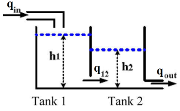
Controlling the liquid levels between tanks is a major challenge in the process industries. Liquid must be pumped, stored in tanks, and then pumped to another tank in several industrial processes. Consider the system shown in Figure 1, consisting of two connected tanks [13].
Figure 1. Interconnected twin-tanks system
$q_{{in}}(\frac{c m^3}{s})$ is the Tank 1's flow rate, $q_{12}(\frac{c m^3}{s})$ is the flow rate form Tank 1 to Tank 2, an $q_o(\frac{c m^3}{s}) \mathrm{d}$ is the flow rate of Tank 2. Tanks 1 and 2 have liquid levels at $h_1(c m)$ and $h_2(c m)$, respectively. Both tanks have a cross-sectional size of $A\left(c m^2\right)$. The coupling orifice's area is $a_{12}$, while the output orifice's area is $\mathrm{a}_2$. The cross-sectional area of Tank 1 and the differential between the input and exit flow rates determine how much water accumulates in Tank 1 [4]:
$\dot{h}_1=\frac{q_{i n}-q_{12}}{A}$ (1)
The following is the nonlinear dynamical equation for the flow rate from Tank 1 to Tank 2 [5]:
$q_{12}=a_{12} \sqrt{2 g\left(h_1-h_2\right)}$ (2)
where, the gravitational constant is denoted by g.
Similar to Tank 1, the water accumulation in Tank 2 is determined by [10]:
$\dot{h}_2=\frac{q_{12}-q_o}{A}$ (3)
The flow rate from Tank 2 is given by the following equation [5]:
$q_o=a_2 \sqrt{2 g h_2}$ (4)
Substituting Eq. (2) into Eq. (1) and Eq. (4) into Eq. (3) results in:
$\dot{h}_1=\frac{q_{i n}-a_{12} \sqrt{2 g\left(h_1-h_2\right)}}{A}$ (5)
$\dot{h}_2=\frac{a_{12} \sqrt{2 g\left(h_1-h_2\right)}-a_2 \sqrt{2 g h_2}}{A}$ (6)
Let's assume: $x_1=h_2, c_1=\frac{a_2 \sqrt{2 g}}{A}, c_2=\frac{a_{12} \sqrt{2 g}}{A}, x_2=h_1-h_2$ and $u=q_{i n}$, Eqs. (5) and (6) can be rewritten:
$\dot{x}_1=-c_1 \sqrt{x_1}+c_2 \sqrt{x_2}$ (7)
$\dot{x}_2=\frac{u}{A}-2 c_2 \sqrt{x_2}+c_1 \sqrt{x_1}$ (8)
The mathematical equation of the system is transformed into an equivalent canonical representation, typically expressed as a single nonlinear differential equation, to aid in controller design. Consequently, the system's new coordinates are defined as follows: $z_1$ and $z_2$ are $x_1$ and $\dot{x}_1$ respectively. As a result, the corresponding model's differential equations in new model can be written as follows:
$\dot{z}_1=z_2$ (9)
$\dot{z}_2=f(x)+g(x) u$ (10)
$f(x)=\left(\frac{c_1{ }^2-2 c_2{ }^2}{2}\right)+\frac{c_2 c_1}{2}\left(\frac{\sqrt{z_1}}{\sqrt{x_3}}-\frac{\sqrt{x_3}}{\sqrt{x_1}}\right)$ (11)
$g(x)=\frac{C_2}{2 A \sqrt{x_3}}$ (12)
An essential component of the automation system is the feedback controller. Many control algorithms have been developed for a variety of control systems [14, 15]. This section outlines the process for using two nonlinear control techniques to determine the control law for the coupled-tank system: FL-PD controllers and SMC. These methods are suitable because they effectively manage the nonlinear behaviour, enabling fast and stable liquid-level regulation while maintaining robustness against disturbances.
3.1 Sliding mode control
One well-known robust and systematic controller design is SMC [16, 17]. There are two phases to it. The design of an appropriate sliding surface is the first step, followed by the development of a control law that ensures the system remains on the sliding surface [18]. The sliding surface is defined as follows:
$s=\dot{e}+a_{s m c} e$ (13)
where, $a_{s m c}>0$ is a tuning parameter, and e is the difference between the desired output $z_d$ and the measured output $z_1$.
Calculating the sliding surface's first derivative results in:
$\dot{s}=\ddot{e}+a_{s m c} \dot{e}=\ddot{z}_d-\dot{z}_2+a_{s m c} \dot{e}$ (14)
Substitute $\dot{z}_2$ from Eq. (10) into (14), obtaining:
$\dot{s}=\ddot{z}_d-f(x)-g(x) u+a_{s m c} \dot{e}$ (15)
The second component of the SMC law is the switching term, which generates the discontinuous control action required to drive the system toward and maintain it on the sliding surface [19]. The sliding condition is ensured by designing the switching control such that the derivative of the sliding surface converges to zero. The switching control must make the right decision to prevent chattering in SMC. The power rate reaching law, which is given by Eq. (16) [20], is selected to serve as the switching control.
$\dot{s}=-k_{s m c}|s|^\gamma \operatorname{sgn}(s)$ (16)
where, $\gamma$ is an adjusted parameter between $[0,1], k_{s m c}$ is an adjusted parameter >0, and $s g n$ is the sign function. Setting Eq. (15) yields the final $u$, which is equal to Eq. (16) as follows:
$\ddot{z}_d-f(x)-g(x) u+a_{s m c} \dot{e}=-k_{s m c}|s|^\gamma \operatorname{sgn}(s)$ (17)
To determine the SMC's control law, reorder Eq. (17) as follows:
$u_{s m c}=\frac{1}{g(x)}\left(\ddot{z}_d-f(x)+a_{s m c} \dot{e}+k_{s m c}|s|^\gamma \operatorname{sgn}(s)\right)$ (18)
Stability Proof: let choose Lyapunov function as $V(s)=$ $\frac{1}{2} s^2$. The time derivate of $V$ gives: $\dot{V}=s \dot{s}$. Substitute $\dot{\mathrm{s}}$ as given in Eq. (16) yields $\dot{V}=s\left(-k_{s m c}|s|^\gamma \operatorname{sgn}(s)\right)$. The term $(s \times \operatorname{sgn}(s))$ is equivalent to $(|s|)$. The results of $\dot{V}=$ $-k_{s m c}|s|^{\gamma+1}$. For $\gamma>-1$ and $k_{s m c}>0$ the $\dot{V}<0$. Thus, the sliding variable s is asymptotically stable.
3.2 Feedback linearization-based proportional-derivative controller
One of the most widely researched techniques for designing trajectory-tracking controllers for nonlinear systems is FL [21, 22]. The nonlinear system is converted into an equivalent linear form by the control law in FL in the manner described below [23]:
$u=\frac{1}{g(x)}\left(-f(x)+u_v\right)$ (19)
where, $g(x)$ and $f(x)$ are the input gain and the state dynamic function, respectively. Any linear controller can be used as the control action $u_v$. The proportional-derivative (PD) control law chosen for this paper is as follows:
$u_v=k_p\left(z_r-z_1\right)+k_d\left(\dot{z}_r-\dot{z}_1\right)$ (20)
where, the controller gains, $k_p$ and $k_d$ are designed to achieve the desired tracking performance.
Due to their ability to solve complex optimization problems, nature-inspired optimization techniques play a prominent role in modern applications [24-27]. In this paper, the CSA, introduced by Askarzadeh [28], is presented to obtain the controller parameters for the SMC and the FL-PD controller.
Crows, members of the corvid family, are among the most intelligent birds. Their cognitive abilities include tool use, face recognition, effective communication, self-awareness, and long-term memory of food locations [29]. Crows can steal food by observing its hiding place and later relocate their own caches to avoid theft. Their experience as thieves helps them anticipate and prevent food pilfering [30].
Based on the population's metaheuristic algorithm, CSA is constructed using the previously mentioned intelligent characteristics. The fundamentals of CSA are as follows:
•Crows live in a flock.
•Crows remember their hiding areas.
•Crows pursue each other to commit theft.
•Crows defend their caches from theft using likelihood.
The model assumes a d-dimensional environment with several crows. The total number of crows in the flock is $N$, and the position of the i crow at a given time (or iteration) iter in the search space is d by a vector. $x^{i,{ iter }}(i=1,2, \ldots$, $N$; $iter =1,2, \ldots$, where $x^{i, i t e r}=\left[x_1^{i, i t e r}, x_2^{i, i t e r}, \ldots, x_d^{i, i t e r}\right]$ and $i t e r_{\text {max }}$ is the highest number of iterations. Crows have a memory for where they hide. The crow's hiding position is indicated by $m^{i, i t e r}$ at iteration iter. To date, this is the most favorable position the crow has attained. Crows recall their most memorable moments. Crows move around and hide in various places in search of food.
Assume that crow $j$ wants to go to its hiding place at iteration iter $m^{j, i t e r}$. Crow $i$ accompanies crow $j$ to his hiding place in this iteration. There are two possible states in this scenario:
State 1: Crow $j$ is unaware that crow $i$ is observing it. As a consequence, crow $i$ will try to reach crow $j$ hiding location. In this situation, the new position of trow $i$ is [31]:
$x^{i, i t e r+1}=x^{i, i t e r}+r_i \times f l^{i, i t e r} \times\left(m^{j, i t e r}-x^{i, i t e r}\right)$ (21)
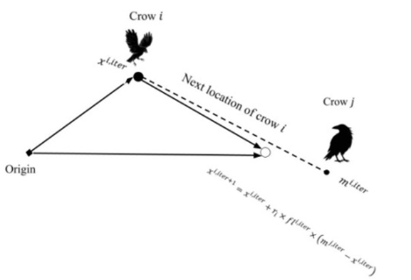
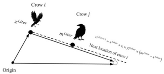
where, $r_i$ is an arbitrary number with a uniform distribution from 0 to 1 and $f l^{\text {i,iter }}$ indicates the journey duration of the crow i at iteration iter. Figure 2 illustrates how $f l$ affects the search capacity. Smaller $f l$ values result in local searches around $x^{i, i t e r}$, while larger values result in global searches farther away. Figure 2(a) demonstrates that if $f l$ is less than 1, crow $i$ moves to the dashed line between $x^{i, i t e r}$ and $m^{j, i t e r}$. In Figure 2(b), selecting a value of $f l$ Greater than 1 results in crow $i$ moving to the dashed line, which may surpass $m^{j, i t e r}$.
Figure 2. Flowchart for state 1 in crow search algorithm (CSA) (a) $f l<1$ and (b) $f l>1$
State 2: Crow j detects that crow i is following it and deceives it by flying to a new search-space location. Thus, the two states can be summarized as follows:
$x^{i, i, t e r+1}=\left\{\begin{array}{lr}x^{i, i, t e r}+r_i \times f l^{i, i t e r} \times\left(m^{j, i t e r}-x^{i, i t e r}\right) \quad r_j \geq A P^{j, i t e r} \\ \text { a random position } \quad \text {otherwise}\end{array}\right.$ (22)
In this formula, $A P^{j, i t e r}$ denotes the awareness probability (AP) of crow $j$ at iteration iter, while $r_i$ is a uniformly distributed random number in the interval $[0,1]$.
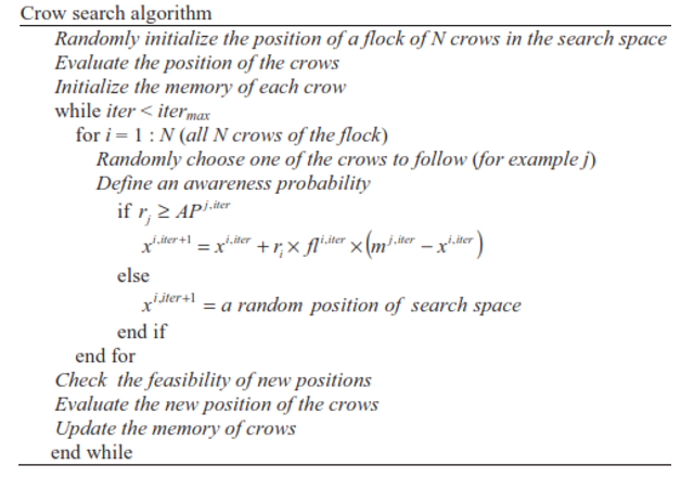
Metaheuristic algorithms must achieve an optimal balance between diversity and intensity. The AP parameter controls intensity and diversity in CSA models. When the AP decreases, CSA searches for a good solution in the area of interest. Using reduced AP values result in increased intensity. However, increasing awareness reduces the likelihood of searching for existing good solutions. CSA typically explores randomizing the search spot globally. Using high AP values lead to increased diversity. Figure 3 depicts the pseudocode for CSA.
Figure 3. Pseudocode for the crow search algorithm (CSA)
The illustrated steps for executing CSA are as follows:
Step 1: Establish the problem and specify the parameters that can be changed. This entails defining the constraints, decision variables, and optimization objectives. The flock size (N), the maximum number of iterations ($iter_{max}$), the flight length (fl), and the AP are the crucial parameters to select for the CSA.
Step 2: Initialize the crows’ positions and memory.
The N crows that make up the flock are dispersed at random throughout a d-dimensional search space. d denotes the number of characteristics considered, and each crow represents a potential solution to the issue.
$\text{Crows} =\left[\begin{array}{cccc}x_1^1 & x_2^1 & \cdots & x_d^1 \\ x_1^2 & x_2^2 & \cdots & x_d^2 \\ \vdots & \vdots & \vdots & \vdots \\ x_1^N & x_2^N & \cdots & x_d^N\end{array}\right]$ (23)
Each crow memory is initialized. During the first iteration, the crows are presumed to have buried their food at their initial locations due to their lack of experience.
$\text{Memory} =\left[\begin{array}{cccc}m_1^1 & m_2^1 & \cdots & m_d^1 \\ m_1^2 & m_2^2 & \cdots & m_d^2 \\ \vdots & \vdots & \vdots & \vdots \\ m_1^N & m_2^N & \cdots & m_d^N\end{array}\right]$ (24)
Step 3: Determine fitness (target) function.
To determine the quality of a crow's position, the selected parameters are added to the objective function.
Step 4: Establish a new position.
In the search area, crows take up new places in the following ways: Let's say crow wants to take on a new role. To locate the hidden food by the crow $m^j$. This crow randomly chooses one of the flock of crows, such as crow j. Eq. (21) determines the new location of crow i. The procedure is repeated for each crow.
Step 5: Evaluate the viability of new locations.
Each crow's new location is assessed for viability. The crow updates its region if it can reach the new place. On the other hand, the crow stays where it is.
Step 6: Assess the fitness function of new locations.
The fitness of each crow’s new position is evaluated.
Step 7: Update memory.
Each crow then updates its memory based on the new position.
$x^{i, i t e r+1}=\left\{\begin{array}{cc}x^{i, i t e r+1} & f\left(x^{i, i t e r+1}\right) \text { is better than } f\left(m^{i, i t e r}\right) \\ m^{i, i, \text { ter }} & \text { otherwise }\end{array}\right.$ (25)
where, $f(.)$ is the desired function output. When a crow's new position exceeds the previously memorized position in terms of fitness function value, it adjusts its memory to reflect the new location.
Step 8: Check the termination requirements.
Steps four to seven continue until $iter_{max}$ has been reached. Once the termination requirement is met, the optimal memory position is identified based on the objective function value.
MATLAB simulations were used to implement and assess FL-PD and SMC controllers for the closed-loop coupled-tank system. Table 1 [10] is a list of the primary system parameters employed in the investigation. The beginning level of Tank 2 was 0.01 cm, while the target level was 5 cm. The physical actuator constraint saturates in the range of 0 to 150 cm3/s for the input flow rate.
Table 1. Twin-tank system parameters
|
Parameters |
Values |
|
Cross-sectional area (A) |
200 cm2 |
|
Gravitational constant (g) |
981 cm/s2 |
|
Area of the outlet orifice ($a_2$) |
0.25 cm2 |
|
Area of the coupling orifice ($a_{12}$) |
0.6 cm2 |
To guarantee fair comparison, the CSA is used to adjust each controller's tuning parameters ($a_{s m c}$ and $k_{s m c}$ in Eq. (18) for the SMC and ($k_p$ and $k_d$) in Eq. (20) for the PD. The root sum of squared error (RSSE), as defined in Eq. (26) [32], is an error index that the CSA used to improve the performance of the two controllers. The RSSE measure is often used to evaluate control performance.
$R S S E=\sqrt{\sum_{m=1}^n e_m^2}$ (26)
where, $e_m$ is the tracking error in each sample m, and n is the simulation's total sample count. The population size (N) is 25, there are 40 iterations (itermax), the AP is 0.1 and the flight length (fl) is 2 in the CSA. Table 2 reports the controllers' ideal values by CSA.
Table 2. The ideal tuning parameter values for the controllers based on crow search algorithm (CSA)
|
Controller |
Parameters |
Values |
|
SMC |
$a_{s m c}$ |
0.7 |
|
$k_{s m c}$ |
2.8 |
|
|
$\gamma$ |
0.9 |
|
|
FL-PD |
$k_p$ |
0.42 |
|
$k_d$ |
0.8 |
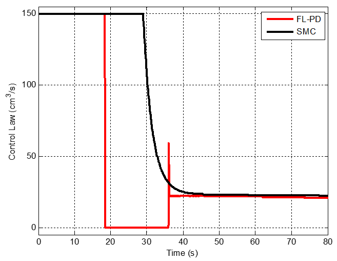
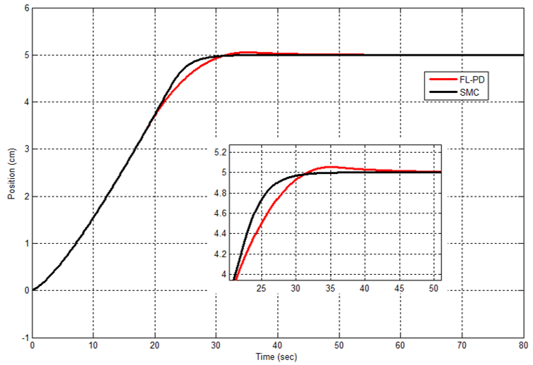
The control law and the response of the two controlled systems are depicted in Figures 4 and 5, respectively. The equivalent dynamic performance numerical value is shown in Table 3.
As shown in Figure 4, the control input remains within the actuator’s operating limits and the SMC signal is free from significant chattering. Furthermore, Figure 5 shows that the SMC controller outperforms the FL-PD. The numerical information in Table 3 shows that for the FL-PD, the settling time ($t_s$) is 27 seconds; for the SMC, it is 25 seconds. Furthermore, FL-PD controller exhibits a 5.5% overshoot, while the SMC eliminates overshoot, demonstrating improved transient performance. Additionally, the SMC controller's RSSE index value (50.54 cm) is lower than the FL-PD controller's RSE index value (50.67 cm).
Figure 4. Sliding mode control (SMC) and feedback linearization-based proportional-derivative (FL-PD) control signals with actuator saturation
Figure 5. The system's response based on sliding mode control (SMC) and feedback linearization-based proportional-derivative (FL-PD) under normal operation
Table 3. Comparison of dynamic performance under normal operation
|
Index |
SMC |
FL-PD |
|
RSSE (cm) |
50.54 |
50.67 |
|
$t_s$ (s) |
25 |
27 |
|
Overshoot (%) |
0 |
5.5 |
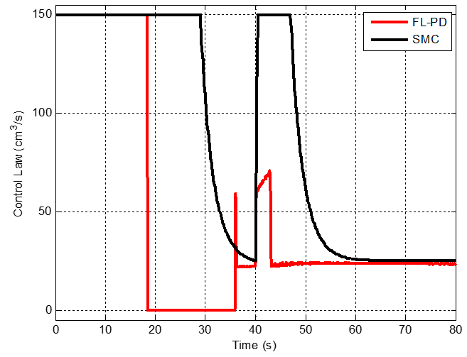
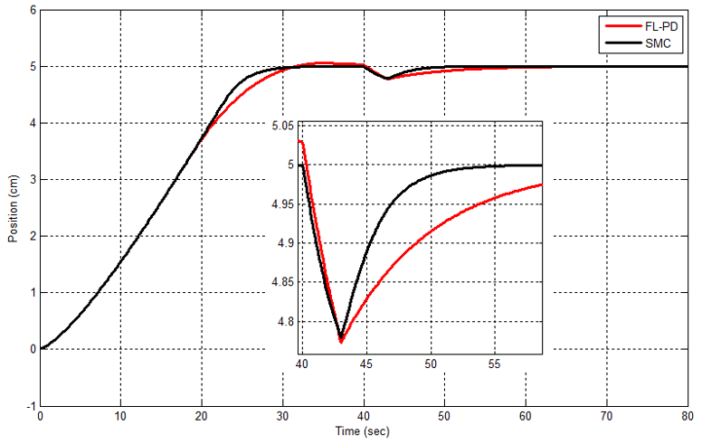
After 40 seconds of simulation time, a step disturbance with an amplitude of 20% of the input reference was injected into the level of Tank 2 to assess each controller's ability to reject disturbances. The control laws and the output responses of both controlled systems under disturbance conditions are shown in Figures 6 and 7. Additionally, the control performance was evaluated using the RSSE criterion, recovery time (trec) and post-disturbance steady-state error (esspd). Table 4 displays the corresponding dynamic responses of the two controllers.
Figure 6. Sliding mode control (SMC) and feedback linearization-based proportional-derivative (FL-PD) control signals with actuator saturation under disturbance
Figure 7. The system's response based on sliding mode control (SMC) and feedback linearization-based proportional-derivative (FL-PD) under disturbance
Table 4. Comparison of dynamic performance under disturbance
|
Index |
SMC |
FL-PD |
|
RSSE (cm) |
50.55 |
50.69 |
|
$t_{r e c}$ (s) |
5 |
9 |
|
$e s s_{p d}$ (cm) |
0 |
0.0013 |
It is evident from comparing the SMC and FL-PD's performance in Figure 7 and Table 4 that the SMC's disturbance rejection reduces deviations more effectively than the FL-PD's. For the FL-PD, the RSSE number is 50.69; for the SMC, it is 50.55. Moreover, the trec for the SMC (5 s) is less than the FL-PD (9 s). Additionally, the esspd is 0.0013, whereas the SMC effectively rejects the disturbance and restores the tracking error to zero.
Based on the results obtained under both normal operating conditions and in the presence of external disturbance, it can be concluded that the SMC provides superior overall performance compared with the FL-PD, particularly in terms of tracking accuracy and disturbance rejection.
This study compared SMC with an FL-PD controller for a coupled-tank system. The mathematical model of the system was constructed, and the method for developing the two controllers was given. The CSA technique was used to modify the modifiable parameters of the proposed controllers. MATLAB was used to program the system with the two optimal controllers. The SMC was found to have superior control characteristics compared to FL-PD control, as indicated by the simulated results. Comparing the suggested CSA with other optimization algorithms and/or employing other nonlinear controllers, this study could be expanded for future research. Additionally, this paper could be extended by experimental validation or consideration of other additional practical factors such as sensor noise, pump dynamics, and measurement delays. Moreover, in order to assess the success of the suggested control technique in larger and more difficult process control systems, future research may concentrate on expanding it to more intricate multi-tank arrangements.
[1] Gouta, H., Said, S.H., Barhoumi, N., M'Sahli, F. (2015). Observer-based backstepping controller for a state-coupled two-tank system. IETE Journal of Research, 61(3): 259-268. https://doi.org/10.1080/03772063.2015.1018846
[2] Pan, H.Z., Wong, H., Kapila, V., de Queiroz, M.S. (2005). Experimental validation of a nonlinear backstepping liquid level controller for a state-coupled two-tank system. Control Engineering Practice, 13(1): 27-40. https://doi.org/10.1016/j.conengprac.2003.12.019
[3] Fellani, M.A., Gabaj, A.M. (2015). PID controller design for two tanks liquid level control system using Matlab. International Journal of Electrical and Computer Engineering, 5(3): 436-442. https://doi.org/10.11591/ijece.v5i3.pp436-442
[4] Chauhan, S., Singh, B., Singh, M. (2021). Modified ant colony optimization based PID controller design for coupled tank system. Engineering Research Express, 3(4): 045005. https://doi.org/10.1088/2631-8695/ac2bf3
[5] Mien, T.L. (2017). Liquid level control of coupled-tank system using fuzzy-PID controller. International Journal of Engineering Research and Technology, 6(11): 459-464.
[6] Awelewa, A., Ojo, K., Abimbola-Oladejo, T., Owolabi, T. (2025). Fuzzy-PID controller for liquid level control of tank systems. NIPES-Journal of Science and Technology Research, 7(2): 2794-2801. https://doi.org/10.37933/nipes/7.4.2025.SI332
[7] Toms, T., Hepsiba, D. (2014). Comparison of PID controller with a sliding mode controller for a coupled tank system. International Journal of Engineering Research and Technology, 3(2): 151-154.
[8] Parvat, B.J., Jadhav, V.K., Lokhande, N.N. (2012). Design and implementation of sliding mode controller for level control. IOSR Journal of Electronics and Communication Engineering, 2: 51-54.
[9] Nandhinipriyanka, G., Ishwarya, S., Janakiraman, S., Thana, C.S., Vaishali, P. (2018). Design of model reference adaptive controller for cylinder tank system. International Journal of Pure and Applied Mathematics, 118(20): 2007-2013.
[10] Delavari, H., Noiey, A.R. (2007). Genetic-based fuzzy sliding mode control of an interconnected twin-tanks. In EUROCON 2007-The International Conference on "Computer as a Tool", Warsaw, Poland, pp. 714-719. https://doi.org/10.1109/EURCON.2007.4400597
[11] Khalid, M.U., Kadri, M.B. (2012). Liquid level control of nonlinear coupled tanks system using linear model predictive control. In 2012 International Conference on Emerging Technologies, Islamabad, Pakistan, pp. 1-5. https://doi.org/10.1109/ICET.2012.6375434
[12] Mfoumboulou, Y.D. (2021). Design of a model reference adaptive PID control algorithm for a tank system. International Journal of Electrical and Computer Engineering (IJECE), 11(1): 300-318.
[13] Delavari, H., Ghaderi, R., Ranjbar, A., Momani, S. (2010). Fuzzy fractional order sliding mode controller for nonlinear systems. Communications in Nonlinear Science and Numerical Simulation, 15(4): 963-978. https://doi.org/10.1016/j.cnsns.2009.05.025
[14] Al-Ali, M.A., Lutfy, O.F., Al-Khazraj, H. (2024). Investigation of optimal controllers on dynamics performance of nonlinear active suspension systems with actuator saturation. Journal of Robotics and Control (JRC), 5(4): 1041-1049. https://doi.org/10.18196/jrc.v5i4.22139
[15] Wang, Q.G., Sun, J.T., Zhang, J.X., et al. (2023). Survey of transient performance control. Control Engineering Practice, 138: 105559. https://doi.org/10.1016/j.conengprac.2023.105559
[16] Hasan, A.F., Nawfal, M., Al-Araji, A.S., Al-Khazraji, H., Humaidi, A.J. (2025). Improved sliding mode control for maximum power point tracking in solar photovoltaic applications under varying conditions. International Journal of Robotics and Control Systems, 5(3): 1790-1807. https://science-eprint.org/id/eprint/329/.
[17] Hamzah, M., Majeed, L., Al-Araji, A.S., Dulaimi, H., Al-Khazraji, H. (2026). Sliding mode control based whale optimization algorithm for Duffing oscillator. International Journal of Robotics and Control Systems, 6(1): 495-506. https://pubs2.ascee.org/index.php/IJRCS/article/view/2451.
[18] Qiao, N., Wang, L.H., Liu, M.J., Wang, Z.X. (2022). Sliding mode controller with improved reaching law for harvesting robots. Journal of Intelligent & Robotic Systems, 104(1): 9. https://doi.org/10.1007/s10846-021-01536-6
[19] Ahmed, A.K., Majeed, L.K., Al-Wais, S., Al-Khazraji, H. (2026). Sliding mode position tracking control-based waterwheel plant algorithm for elbow rehabilitation systems. International Journal of Robotics and Control Systems, 6(2): 1164-1180. https://science-eprint.org/id/eprint/1188.
[20] Farhan, N.D., Naji, R.K., Musa, M.K., et al. (2026). Sliding mode based circle search algorithm for inventory control with extended state observer. Buletin Ilmiah Sarjana Teknik Elektro, 8(3): 887-900. https://doi.org/10.12928/biste.v8i3.16220
[21] Vesović, M., Jovanović, R., Trišović, N. (2022). Control of a DC motor using feedback linearization and gray wolf optimization algorithm. Advances in Mechanical Engineering, 14(3): 1-16. https://doi.org/10.1177/16878132221085324
[22] Hache, A., Thieffry, M., Yagoubi, M., Chevrel, P. (2022). Control-oriented neural state-space models for state-feedback linearization and pole placement. In 2022 10th International Conference on Systems and Control (ICSC), Marseille, France, pp. 429-434. https://doi.org/10.1109/ICSC57768.2022.9993820
[23] Al-Ani, F.R., Lutfy, O.F., Al-Khazraji, H. (2025). Optimal synergetic and feedback linearization controllers design for magnetic levitation systems: A comparative study. Journal of Robotics and Control (JRC), 6(1): 22-30. https://doi.org/10.18196/jrc.v6i1.24452
[24] Khlil, S., Al-Khazraji, H., Alabacy, Z. (2020). Solving assembly production line balancing problem using greedy heuristic method. In the Fourth Scientific Conference for Engineering and Postgraduate Research, Baghdad, Iraq, 745(1): 012068. https://doi.org/10.1088/1757-899X/745/1/012068
[25] Kadhim, M.Q., Yaseen, F.R., Al-Khazraji, H., Humaidi, A.J. (2024). Application of terminal synergetic control based water strider optimizer for magnetic bearing systems. Journal of Robotics and Control (JRC), 5(6): 1973-1979. https://doi.org/10.18196/jrc.v5i6.23867
[26] Abdulkareem, A.I., Dhahad, H.A., Yousif, N.Q. (2018). Prospect theory in particle swarm optimization for constrained nonlinear optimization problems. In 2018 Third Scientific Conference of Electrical Engineering (SCEE), Baghdad, Iraq, pp. 144-149. https://doi.org/10.1109/SCEE.2018.8684144
[27] Dafid, A., Sudianto, A.I., Thinakaran, R., et al. (2025). Optimizing K-nearest neighbors with particle swarm optimization for improved classification accuracy. Jurnal Ilmiah Teknik Elektro Komputer dan Informatika (JITEKI), 11(2): 238-250. https://journal.uad.ac.id/index.php/JITEKI/article/view/30775.
[28] Askarzadeh, A. (2016). A novel metaheuristic method for solving constrained engineering optimization problems: crow search algorithm. Computers & Structures, 169: 1-12. https://doi.org/10.1016/j.compstruc.2016.03.001
[29] Sadollah, A., Bahreininejad, A., Eskandar, H., Hamdi, M. (2013). Mine blast algorithm: A new population based algorithm for solving constrained engineering optimization problems. Applied Soft Computing, 13(5): 2592-2612. https://doi.org/10.1016/j.asoc.2012.11.026
[30] Prior, H., Schwarz, A., Güntürkün, O. (2008). Mirror-induced behavior in the magpie (Pica pica): Evidence of self-recognition. PLoS Biology, 6(8): e202. https://doi.org/10.1371/journal.pbio.0060202
[31] Alkrwy, A., Hussein, A.A., Atyia, T.H., Khamees, M. (2021). Adaptive tuning of PID controller using crow search algorithm for DC motor. In 2nd International Scientific Conference of Engineering Sciences (ISCES 2020), Diyala, Iraq, 1076(1): 012001. https://doi.org/10.1088/1757-899X/1076/1/012001
[32] Yi, H., Zhang, Q.Y. (2020). An optimal fuzzy control method for nonlinear time-delayed batch processes. IEEE Access, 8: 42608-42618. https://doi.org/10.1109/ACCESS.2020.2976869