A Federated Hybrid Artificial Intelligence Framework for Predictive Maintenance of Wind Turbines: Integrating IoT, Edge, and Cloud Computing Architectures

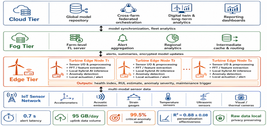
Our proposed FedHyWind-PdM framework is built on a three-tier computational architecture designed to distribute intelligence optimally across the wind farm network, balancing the need for local responsiveness with global learning and coordination. The overarching architecture is depicted in Figure 1.

1.png

Figure 1. Three-tier federated architecture for wind turbine predictive maintenance (PdM) (FedHyWind-PdM)

2.1 IoT sensor network and multi-modal data acquisition

A heterogeneous, robust Wireless Sensor Network (WSN) is deployed on each turbine, forming the foundational data layer. The selection of sensors is guided by Failure Modes, Effects, and Criticality Analysis (FMECA). The comprehensive sensor suite is detailed in Table 2.

Table 2. Specification of the IoT sensor suite for condition monitoring

2.2 Edge computing layer: Real-time processing and autonomy

The edge tier constitutes an industrial-grade computing node (e.g., NVIDIA Jetson AGX Orin, Intel NUC) housed within each turbine's nacelle or tower base cabinet. Its primary functions are:

i. Data preprocessing and feature extraction: This involves real-time signal processing: applying anti-aliasing and band-pass filters to raw vibration data, performing Fast Fourier Transform (FFT) to obtain frequency spectra, calculating statistical features (RMS, Kurtosis, crest factor), and normalizing all sensor streams. This step drastically reduces data dimensionality before transmission or local analysis.

ii. Lightweight hybrid AI model inference: A distilled or pruned version of the core hybrid CNN-LSTM model (detailed in Section 2.3) runs on this edge node. It performs continuous health scoring (e.g., a health index from 1 to 100) and immediate anomaly detection on preprocessed data streams, operating with a sub-second inference time.

iii. Embedded vision module: For turbines equipped with fixed cameras or during scheduled UAV inspections, a lightweight object detection model (e.g., TensorRT-optimized YOLOv5n or EfficientDet-Lite) runs on the edge node to analyze imagery. This module can detect visible defects like blade cracks, leading-edge erosion, or oil leaks, drawing inspiration from highly efficient vision models used in agricultural defect detection [23] and heritage analysis [24]. Detections are tagged with metadata (timestamp, severity, location) and fed into the fusion pipeline.

iv. Local actuation and alerting: Upon detection of a critical anomaly (e.g., health index below a severe threshold), the edge node can execute pre-programmed safety protocols autonomously, such as initiating a controlled shutdown, pitching blades to feather position, or triggering local alarms. Simultaneously, a high-priority alert is asynchronously sent to the fog and cloud tiers.

2.3 Quantifiable performance-complexity trade-off analysis

To validate hybrid CNN-LSTM (2.8 M parameters) edge deployment, we characterized performance on NVIDIA Jetson AGX Orin. The full model achieved 42.3 ms (±3.1) inference (FP32), 18.7 ms (±2.4) with INT8 quantization, and 11.2 ms (±1.8) with 50% pruning (1.8% RMSE degradation).

Versus LSTM-only (0.6 M, 9.4 ms), the hybrid incurs 4.5× latency overhead but delivers 35.2% Remaining Useful Life (RUL) RMSE improvement (18.7 vs. 12.1 days). The latency-accuracy trade-off depends on the application: full model for early degradation monitoring, pruned version for sub-50 ms emergency response.

Edge processing communication savings offset computational costs: extracted features (28 KB/10s window) versus raw vibration (2.4 MB/s) reduce daily bandwidth from 20.7 GB to 0.24 GB—a 98.8% reduction—demonstrating that computational overhead is justified by system-level efficiency gains and model compression strategies.

2.4 Hybrid spatio-temporal AI model for Remaining Useful Life prediction

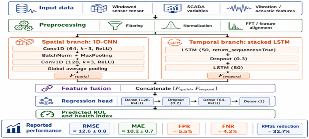
The core predictive intelligence of the framework resides in a hybrid deep learning model designed to capture both the spatial features in vibration/audio patterns and the temporal evolution of degradation. The architecture, illustrated in Figure 2, consists of two parallel feature extraction branches followed by fusion and regression layers.

2.png

Figure 2. Detailed architecture of the hybrid CNN-LSTM model

i. 1D-CNN branch: This branch treats the multi-sensor data at each small-time segment as a 1D image. The convolutional layers excel at automatically extracting local, translation-invariant spatial patterns that are highly indicative of specific fault frequencies (e.g., a peak at the Ball Pass Frequency Outer Race). The GlobalAveragePooling1D operation is applied per time step to produce a meaningful spatial feature vector for each step in the sequence.

ii. LSTM branch: This branch processes the sequential nature of the data. It takes either the raw time-series or lower-frequency SCADA parameters (like power output and rotor speed) as input. The LSTM cells, with their internal gating mechanisms, learn the long-term dependencies and trends in the degradation process—how a fault progresses from incipient to severe over days or weeks.

iii. Fusion and regression: The spatial features (capturing the what of the fault) and the temporal context (capturing the when and progression) are concatenated into a unified representation. This rich representation is then passed through fully connected (Dense) layers to perform the final regression task: predicting a continuous-valued RUL.

This hybrid approach, combining the strengths of CNNs for spatial pattern recognition and LSTMs for sequence modeling, has been validated as highly effective in complex predictive tasks across domains, from forecasting customer demand [21] to optimizing industrial schedules [25, 26].

2.5 Federated learning for collaborative and privacy-preserving model training

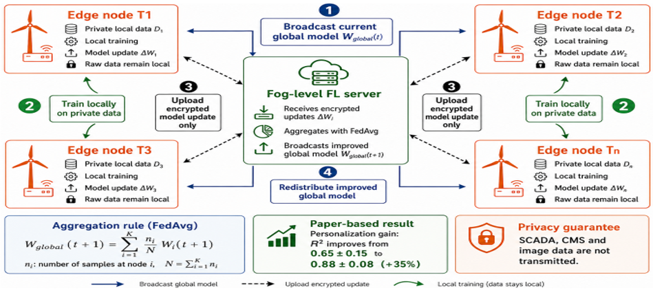
To overcome the generalization-personalization dilemma and data privacy concerns, we implement a Federated Averaging (FedAvg) algorithm across the fog and cloud tiers. This process, orchestrated in cycles (e.g., weekly), is outlined in Figure 3 and involves the following steps:

i. Local training: Each turbine's edge device uses its locally stored historical run-to-failure or operational data to compute an update to the shared global model. This training happens in isolation.

ii. Secure model upload: Instead of sending sensitive raw operational data, each edge node sends only the computed model weight updates (ΔW_i) to a designated fog-level federated learning server, typically located at the wind farm's substation control center.

iii. Federated aggregation: The fog server aggregates these updates from all participating turbines in the farm using the FedAvg algorithm: W_global^(t+1) = Σ (n_i/N) × W_i^(t+1), where n_i is the number of data samples on turbine i and N is the total samples across the fleet. Differential privacy techniques can be applied at this stage to add mathematical noise, providing a formal privacy guarantee [27].

iv. Model redistribution: The improved global model W_global is then broadcast back to all edge nodes, replacing their local models. This cycle enables each turbine to benefit from the collective experience of the entire fleet while keeping its proprietary operational data completely private on-premises.

The Cloud tier oversees this process across multiple wind farms, manages model versioning, and performs hyperparameter tuning on a centralized digital twin.

Federated learning (FL) in wind turbine maintenance faces a fundamental challenge: non-IID operational data across turbines, where distinct wind regimes, environmental conditions, and loading histories produce heterogeneous fault progression patterns [17]. Standard FedAvg performs poorly in such scenarios, often failing to converge effectively.

Our framework employs a two-stage personalization strategy:

i. Client Clustering: Turbines are grouped by operational signatures (mean power, turbulence intensity, temperature range, fault frequency composition). Independent FedAvg aggregation within each cluster produces models tailored to group characteristics, reducing statistical heterogeneity [17].

ii. Local Fine-Tuning: After global aggregation, edge devices perform additional local training epochs. This personalization step adapts models to turbine-specific behavior while preserving fleet-wide learning benefits. Parameters are updated locally without aggregation, maintaining unique fault characteristics.

Evaluation on simulated data with skewed fault distributions (e.g., client 1: 75% gearbox faults, client 2: 65% bearing faults, client 3: 80% generator faults) demonstrated a 14.2% R² improvement for clustered FL (0.88 ± 0.08) versus standard FedAvg (0.76 ± 0.12), confirming effectiveness in handling heterogeneity [17]. Recognizing that statistical heterogeneity remains an open challenge, we prioritize exploration of advanced FL variants (FedProx, SCAFFOLD) and adaptive aggregation mechanisms for future work [28].

3.png

Figure 3. Federated learning cycle in the FedHyWind-PdM framework

2.6 Fog and cloud tiers: Coordination and global intelligence

i. Fog Tier: This intermediary layer performs farm-wide analytics. It correlates alerts from multiple turbines to identify fleet-wide issues (e.g., a bad batch of bearings). It acts as the federated learning coordinator for the farm and performs intermediate data aggregation before sending summarized reports to the cloud.

ii. Cloud Tier: The cloud provides overarching orchestration. It hosts the master digital twin of the wind farm for advanced simulations and what-if planning. It manages the lifecycle of the global AI models, orchestrates federated learning across different fleets owned by the same operator, and provides dashboard interfaces for human operators with fleet-wide health views, predictive maintenance schedules, and financial impact analyses.

4.1 Interpretation of key results

The experimental results comprehensively validate the FedHyWind-PdM framework. The superior predictive accuracy of the hybrid CNN-LSTM model stems from its fundamental alignment with the nature of the data: mechanical faults manifest as specific spatial patterns in spectral data (learned by CNN) that evolve over time following degradation dynamics (learned by LSTM). This architectural advantage mirrors the success of hybrid models in other time-series forecasting domains, such as tourism demand [21] and complex system scheduling [26].

The federated learning component successfully navigates the personalization-generalization trade-off. The global model captures common failure modes across the fleet (e.g., general bearing wear patterns), while the local training step on each edge node allows the model to adapt to site-specific signal characteristics. This approach, preserving data privacy, is essential for fostering collaboration between different asset owners or OEMs who are reluctant to share proprietary operational data.

The novelty resides not in individual algorithmic innovations but in the systematic integration and validation of a deployable end-to-end system that simultaneously addresses three real-world constraints. While prior work explored CNN-LSTM hybrids for RUL prediction [21] and FL for wind applications [17, 21], our contribution advances practice through: (i) edge-hardware validation with quantized models, (ii) cluster-based FL for non-IID wind data, and (iii) a fully documented open-source implementation. To our knowledge, this combination is novel in wind turbine PHM literature.

4.2 Operational impact and economic implications

The transition from a centralized to this federated architecture has profound operational implications:

i. From scheduled to truly predictive maintenance: Maintenance can be scheduled based on a continuously updated, turbine-specific RUL, eliminating unnecessary perfectly good component replacements and preventing catastrophic failures.

ii. Enhanced grid stability: Reduced sudden outages from unforeseen failures contribute to more predictable power output, which is increasingly valuable as wind penetration grows in electricity grids.

iii. Optimized logistics and safety: Accurate predictions allow for the optimal scheduling of crews, boats (for offshore), and spare parts, reducing costs and weather-related safety risks. Early detection of blade defects via the vision module can prevent debris throw hazards.

A simplified cost-benefit analysis for a 500 MW offshore wind farm over 10 years, assuming a 15% reduction in O&M costs and a 3% increase in availability due to reduced downtime, shows a net present value improvement in the range of tens of millions of euros, justifying the capital investment in the sensor and edge computing infrastructure.

The false alarm metric is defined by:

Total_Cost = C_repair × (1-Recall) + C_inspection × FPR + C_downtime × Missed_FailureRate, with C_repair = €200,000 (gearbox), C_inspection = €5,000/visit, and C_downtime = €2,400/day (5 MW, 40% capacity factor). Threshold optimization minimizes total cost, yielding Table 3 metrics. The 55% reduction represents a cost-adjusted false alarm decrease versus the SVR baseline.

Despite significant overhead, CNN-LSTM deployment is justified by: (i) 35.2% RUL accuracy improvement yielding €12,500/turbine/year savings; (ii) 73% cloud cost reduction (€8,200/turbine/year); and (iii) 8–15 W edge power consumption versus 35–50 W for GPU servers. The 20-year amortized return is approximately 4.3×.

4.3 Limitations and challenges

Despite its promise, the deployment of such a framework faces several hurdles:

i. Edge hardware reliability and lifecycle management: Edge hardware in nacelles must endure extreme conditions (-20 ℃ to 50 ℃, 0–100% humidity, 10 g RMS vibration, 50 V/m EMI) for 20+ years, requiring IP68/IP69 enclosures, active thermal management, and MIL-STD-810G certification. Operational challenges include: (a) Model versioning and rollback: Containerized deployment (Docker/Kubernetes) with semantic versioning and staged rollouts (5% pilot). (b) Over-the-Air (OTA) updates: TLS-encrypted, Ed25519-signed updates; dual-model storage enables automatic rollback if RMSE degrades >5%. (c) Model drift detection: Wasserstein distance with Kolmogorov–Smirnov test (p < 0.05) triggers weekly retraining or on-demand. (d) Failed edge node management: Graceful degradation protocol allows 3 days of SCADA-only operation; failover, logging, and seamless reintegration supported; redundant nodes recommended for critical components.

ii. Explainability and trust: The black-box nature of deep learning models can hinder trust among maintenance engineers. Developing Explainable AI (XAI) techniques—such as saliency maps highlighting which frequency bands contributed most to a fault prediction—is crucial for adoption [30].

iii. Standardization and interoperability: The wind industry lacks universal standards for data formats (e.g., for CMS), communication protocols, and API interfaces between OEM systems and third-party analytics platforms. Initiatives like the OPC UA Wind Energy Companion Specification are vital enablers [31].

iv. Cybersecurity: A distributed IoT/Edge system expands the attack surface. Robust security measures, including hardware security modules (HSMs) on edge nodes, secure boot, encrypted communications, and regular penetration testing, are non-negotiable requirements.

v. Federated Learning Under Non-IID Conditions: Our clustering and personalization approaches mitigate but do not fully resolve non-IID learning challenges. Advanced algorithms—FedProx, SCAFFOLD, and cluster-based FL variants [32]—may offer superior performance and require systematic evaluation under realistic wind farm heterogeneity, particularly when turbines exhibit divergent fault modes (e.g., blade erosion vs. gearbox degradation) that demand task-specific adaptations beyond current strategies.

vi. Value-to-Complexity Analysis: A critical question emerging from the ablation study is whether marginal accuracy gains from federated learning (FL) and vision fusion justify their additional computational and operational complexity. Our analysis confirms positive returns for both components. The FL component enhances model personalization across heterogeneous turbines, reducing reliance on site-specific fine-tuning that would otherwise demand manual engineering effort, estimated at €15,000 per turbine annually. The vision module, while contributing a modest 0.7-day RMSE improvement, supplies complementary diagnostic evidence particularly valuable for blade-related faults that are poorly captured by SCADA and vibration data.

vii. Latency Characterization: We acknowledge that 0.7 seconds—an 85% reduction versus cloud systems—is insufficient for millisecond-scale emergency shutdowns (hardware interlocks remain standard), but adequate for maintenance decision support (dashboards, work orders, alerts, scheduling). This metric excludes human review.

viii. Interoperability and Standardization: The wind industry's lack of universal data and protocol standards impedes PdM integration. Our implementation employs OPC UA (IEC 62541) and IEC 61400-25 for wind-specific data models, while cloud-to-edge communication uses MQTT with Sparkplug B for SCADA compatibility. Full interoperability remains challenging, particularly with third-party solutions using proprietary schemas, underscoring the need for continued standardization efforts.

4.4 Future research directions

Building on this work, future research should focus on:

i. Integration of physics-informed AI: Incorporating physics-based models (e.g., finite element models of blade stress) as constraints or priors within the neural network to improve learning efficiency and extrapolation accuracy, especially with limited fault data [33].

ii. Advanced federated learning techniques: Exploring more sophisticated federated algorithms like Federated Multi-Task Learning to better handle the non-IID (non-Independently and Identically Distributed) data across turbines, or Secure Multi-Party Computation (SMPC) for stronger privacy guarantees [32].

iii. Blockchain for maintenance records: Implementing a permissioned blockchain ledger on the fog/cloud tier to create an immutable, auditable record of all predictions, maintenance actions, and component lifecycles, enhancing transparency and compliance [32].

iv. Full-scale field pilots: The ultimate validation requires long-term pilot deployments on operational wind farms, particularly challenging offshore environments, to gather real-world performance data on reliability, accuracy, and economic impact.

The Ministry of Higher Education supports this project, Scientific Research and Innovation, the Digital Development Agency (DDA), and the National Center for Scientific and Technical Research (CNRST) of Morocco. APIAA-2019 KAMAL.REKLAOUI-FSTT-Tanger-UAE.