Thi-Mai-Phuong Dao![]() | Sy-Dung Vu
| Sy-Dung Vu![]() | Phan-Duy-Tan Nguyen
| Phan-Duy-Tan Nguyen![]() | Minh-The Do
| Minh-The Do![]() | Duc-Hieu Nguyen
| Duc-Hieu Nguyen![]() | Thi-Duyen Bui
| Thi-Duyen Bui![]() | Mai-Duyen Nguyen
| Mai-Duyen Nguyen![]() | Ngoc-Khoat Nguyen*
| Ngoc-Khoat Nguyen*![]()
© 2026 The authors. This article is published by IIETA and is licensed under the CC BY 4.0 license (http://creativecommons.org/licenses/by/4.0/).
OPEN ACCESS
This paper presents the development of an intelligent control framework for a 5-DOF robotic arm that integrates a Proportional-Derivative (PD)-Fuzzy controller with computer vision techniques for automated waste classification. The kinematic and dynamic models of the robotic arm are formulated using the Denavit-Hartenberg (D-H) convention. The proposed PD-Fuzzy control scheme improves the dynamic behavior of the system by reducing overshoot, decreasing steady-state error, and shortening the settling time when compared with conventional control strategies. The effectiveness of the control approach is verified through simulations performed in MATLAB/Simulink and SolidWorks, which demonstrate stable and reliable robotic operation. In addition, a vision-based classification module is implemented in which a camera captures real-world waste images. The images are processed using a trained YOLOv11 model implemented in the Visual Studio Code environment, and the detected object classes, together with spatial position information are transmitted to MATLAB to generate motion control commands for the robotic arm. The detected object classes and spatial position information are subsequently transmitted to MATLAB to generate motion control commands for the robotic arm. The experimental results demonstrate high classification accuracy, with F1-scores above 0.87 for all classes, while the paper category achieves the highest score of 0.9546. Overall, the proposed system satisfies widely accepted performance criteria for multi-class classification. The primary objective of this study is to develop a vision-based robotic waste-sorting system that enables fast, accurate, and stable operation, thereby improving automation and efficiency in waste management applications.
5-DOF robotic arm, Proportional-Derivative_Fuzzy, simulation, YOLOv11, visual code
The volume of global waste has been increasing at an unprecedented rate, posing serious environmental challenges. Recent estimates indicate that approximately 3.5 million tons of waste are generated worldwide each day. Furthermore, a 2024 report by the United Nations Environment Programme (UNEP) projects that the total amount of municipal solid waste (MSW) will increase significantly, from 2.1 billion tons in 2023 to nearly 3.8 billion tons by 2050 [1].
Vietnam is among the countries with rapidly increasing MSW generation. According to the World Bank, global MSW generation is expected to increase significantly in the coming decades, posing serious environmental challenges if not properly managed [2]. In Vietnam, more than 60,000 tons of MSW are generated each day, with urban areas contributing approximately 60% of the total volume. According to a report by the Vietnam Ministry of Natural Resources and Environment, over 70% of MSW is currently disposed of in landfills, while sanitary landfills account for less than 20% of the total waste treatment methods [3]. These figures highlight the urgent need for more efficient and sustainable waste management strategies.
Currently, Vietnam’s waste-processing sector relies heavily on human labor. Traditional manual sorting practices require substantial effort and time, which restricts the amount of waste that can be handled efficiently. In addition to low productivity, this approach exposes workers to serious occupational hazards, as they must come into direct contact with contaminated and potentially dangerous materials. As waste generation continues to escalate, existing treatment facilities face increasing difficulties in expanding their capacity to meet demand.
In recent years, advancements in artificial intelligence and robotics have introduced promising solutions for waste-sorting processes. The use of robotic arms can replace humans in heavy and hazardous tasks while maintaining continuous, high-throughput operation, thereby improving processing efficiency [4-6]. Since reliable robot control is crucial, this study employs a Proportional-Derivative (PD)-Fuzzy controller to enhance robot performance by improving stability and reducing oscillations in the robotic arm.
The robot kinematic model is formulated using the Denavit–Hartenberg (D-H) convention, which describes the robot structure through parameters such as link dimensions joint angles. Based on this formulation, the dynamic model is derived to determine the forces and torques required for stable joint motion. A PD–Fuzzy controller is then developed, incorporating membership functions and a set of control rules that enable adaptive adjustment under varying operating conditions. Simulation results indicate improved trajectory tracking, faster convergence, and reduced positional error.
For waste detection and classification, materials including Cardboard, Glass, Metal, Paper, and Plastic are recognized using the YOLOv11 algorithm for real-time object detection. Images captured by the camera are processed in Python within the Visual Studio Code environment. Once an object is detected, coordinates obtained from the sensor are transmitted to MATLAB via the UDP protocol, where inverse kinematics is solved to compute the required joint angles for the robotic manipulator.
The combination of a 5-DOF robotic arm and image-processing technology creates a high-performance, stable and efficient system for waste classification. The PD-Fuzzy controller provides flexible and precise robot control, while YOLOv11 offers accurate real-time object detection. The proposed system has the potential to contribute to reducing waste and its environmental impact through efficient classification, serving as an optimal and adaptable solution for waste-management and recycling tasks.
Globally, several advanced waste-sorting robots have been developed with high operational efficiency. Notably, companies such as ZenRobotics have introduced the Fast Picker and Heavy Picker robots, capable of up to 80 picks per minute. AMP Robotics reports that their systems achieve 80–150 picks per minute and process more than 10 billion objects annually. Additionally, ABB has developed the YuMi and IRB 1200 robotic arms, enabling the sorting of waste into four categories ranging from hazardous materials to recyclables Wu et al. [7] presented a robotic system employing deep learning to detect and classify waste in complex environments. Furthermore, Delta-robot architectures combined with Transfer Learning and YOLOv5 have also been successfully applied for real-time plastic-waste classification, demonstrating the central role of AI in enhancing sorting efficiency and speed.
In Vietnam, recent research has increasingly focused on robotic approaches to waste classification, with particular emphasis on the integration of image processing and artificial intelligence techniques. Most projects are limited to theses and small-scale simulations. For example, Pham et al. [8] proposed a waste-sorting system employing a 3-DOF robotic manipulator in conjunction with computer vision methods. The system performs visual-based identification of waste categories and enables automated sorting in practical settings. Meanwhile, 5-DOF robotic arms have received less attention in waste-classification applications compared to 3- DOF or 4-DOF systems.
Traditional Proportional-Integral-Derivative (PID) or Proportional-Derivative (PD) controllers are widely used due to their simple design. Fuzzy systems offer strong adaptability but require the construction of complex rule sets. Recently, the PD-Fuzzy approach has emerged as an effective method, integrating the advantages of PD control (stability and simplicity) and fuzzy logic (flexibility). However, most existing studies remain at the simulation level, with limited real-world experimentation in waste-sorting applications.
Overall, both domestic and international studies reveal significant potential for developing intelligent control systems for 5-DOF robotic arms integrating artificial intelligence in waste-classification tasks. This research direction not only addresses the existing gap in automated waste sorting in Vietnam but also offers strong potential for practical deployment in industrial zones, educational institutions and urban environments.
2.1 Modeling of the 5-DOF robot
2.1.1 Robot parameters
The parameters of the robot manipulator used in the simulations are listed in Tables 1 and 2.
Table 1. Robot parameters
|
Link |
Lengths (m) |
Masses (kg) |
COM Location (m) |
|
1 |
0.05 |
3.196 |
0.04777 |
|
2 |
0.17 |
1.329 |
0.08535 |
|
3 |
0.25 |
0.639 |
0.13617 |
|
4 |
0.185 |
0.186 |
0.11739 |
|
5 |
0.07 |
0.045 |
0.03188 |
|
6 |
0.08 |
0.036 |
0.03638 |
Table 2. Joint ranges
|
Joint |
Minimum Angle (rad) |
Maximum Angle (rad) |
|
1 |
0 |
2$\pi$ |
|
2 |
-0.89$\pi$ |
0.061$\pi$ |
|
3 |
0.011$\pi$ |
0.972$\pi$ |
|
4 |
-0.055$\pi$ |
1.055$\pi$ |
|
5 |
0 |
2$\pi$ |
The moments of inertia (MoI) and the products of inertia (PoI) are both reported so that the full inertia tensor of each link is specified in Tables 3 and 4.
Table 3. Parameters for moment of inertia (MoI)
|
Link |
$I_{x x}\left(\mathrm{kg} \cdot \mathrm{~m}^2\right)$ |
$I_{y y}\left(\mathrm{kg} \cdot \mathrm{~m}^2\right)$ |
$I_{z z}\left(\mathrm{kg} \cdot \mathrm{~m}^2\right)$ |
|
1 |
0.011493 |
0.011493 |
0.01761 |
|
2 |
0.0040035 |
0.0038734 |
0.0044818 |
|
3 |
0.000349 |
0.003925 |
0.004155 |
|
4 |
0.000681 |
0.0000408 |
0.000703 |
|
5 |
0.0000306 |
0.0000305 |
0.0000042 |
|
6 |
0.0000253 |
0.0000185 |
0.000009 |
Table 4. Products of inertia (PoI)
|
Link |
$I_{x y}\left(\mathrm{kg} \cdot \mathrm{~m}^2\right)$ |
$I_{y z}\left(\mathrm{kg} \cdot \mathrm{~m}^2\right)$ |
$I_{x z}\left(\mathrm{kg} \cdot \mathrm{~m}^2\right)$ |
|
1 |
0 |
0 |
0 |
|
2 |
0.0002254 |
0.0000098 |
0.0000249 |
|
3 |
0.00000135e-05 |
0.0000479 |
0.0000084e-04 |
|
4 |
0.0000128 |
0.000001e-04 |
0.0000011e-05 |
|
5 |
0 |
0 |
0 |
|
6 |
0.0000081e-04 |
0.000006e-06 |
0.0000016e-05 |
2.1.2 Forward kinematics
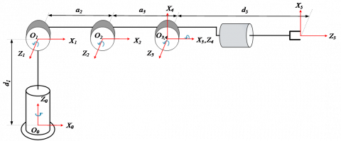
To address the forward kinematics problem, a reference coordinate system is defined at the robot base, followed by local coordinate frames for individual links, as shown in Figure 1. The robot’s kinematic structure is then modeled using the D–H formulation. Through this approach, the spatial position and orientation of the end-effector can be computed with respect to the base reference frame. The associated D–H parameters are summarized in Table 5.
Figure 1. Coordinate frames of the 5-DOF robotic arm
Table 5. Denavit - Hartenberg (D-H) parameter table
|
Link |
$\theta_i$ |
$d_i$ |
$a_i$ |
$\alpha_i$ |
|
1 |
$\theta_1$ |
$d_1$ |
0 |
$90^{\circ}$ |
|
2 |
$\theta_2$ |
0 |
$a_2$ |
0 |
|
3 |
$\theta_3$ |
0 |
$a_3$ |
0 |
|
4 |
$\theta_4$ |
0 |
0 |
$90^{\circ}$ |
|
5 |
$\theta_5$ |
$d_5$ |
0 |
0 |
where,
$\theta_i$ defines the joint rotation that aligns the $x_{i-1}$ axis with the $x_i$ axis through a rotation around the $z_i$ axis.
$d_i$ specifies the linear offset between the $x_{i_{-1}}$ and $x_i$ axes taken along the direction of the axis.
$a_i$ describes the link length, corresponding to the translation from the $z_{i_{-1}}$ axis to the $z_i$ axis along the axis.
$\alpha_i$ indicates the twist angle required to rotate the $z_{i_{-1}}$ axis into alignment with the $z_i$ axis about the $x_i$ axis.
General homogeneous transformation matrix:
${ }^{i-1} T=\left[\begin{array}{cccc}c_i & -s_i c\left(\alpha_i\right) & s_i s\left(\alpha_i\right) & a_i c_i \\ s_i & c\left(\alpha_i\right) c_i & -c_i s\left(\alpha_i\right) & a_i s_i \\ 0 & s\left(\alpha_i\right) & c\left(\alpha_i\right) & d_i \\ 0 & 0 & 0 & 1\end{array}\right]$ (1)
where,
$s_i=\sin \left(\theta_i\right) ; s\left(\alpha_i\right)=\sin \left(\alpha_i\right) ;$
$c_i=\cos \left(\theta_i\right) ; c\left(\alpha_i\right)=\cos \left(\alpha_i\right)$
Transformation matrix from link 1 to link 5:
${ }_1^0 T=\left[\begin{array}{cccc}c_1 & 0 & s_1 & 0 \\ s_1 & 0 & -c_1 & 0 \\ 0 & 1 & 0 & d_1 \\ 0 & 0 & 0 & 1\end{array}\right]$ (2)
${ }_2^1 T=\left[\begin{array}{cccc}c_2 & s_1 & 0 & a_2 c_2 \\ s_2 & c_2 & 0 & a_2 c_2 \\ 0 & 0 & 1 & 0 \\ 0 & 0 & 0 & 1\end{array}\right]$ (3)
${ }_3^2 T=\left[\begin{array}{cccc}c_3 & -s_3 & 0 & a_3 c_3 \\ s_3 & c_3 & 0 & a_3 c_3 \\ 0 & 0 & 1 & 0 \\ 0 & 0 & 0 & 1\end{array}\right]$ (4)
${ }_4^3 T=\left[\begin{array}{cccc}c_4 & 0 & s_4 & 0 \\ s_4 & 0 & -c_4 & 0 \\ 0 & 1 & 0 & 0 \\ 0 & 0 & 0 & 1\end{array}\right]$ (5)
${ }_5^4 T=\left[\begin{array}{cccc}c_5 & -s_5 & 0 & 0 \\ s_5 & c_5 & 0 & 0 \\ 0 & 0 & 1 & d_5 \\ 0 & 0 & 0 & 1\end{array}\right]$ (6)
The end-effector transformation matrix is calculated as follows:
${ }_5^0 T=\left[\begin{array}{cccc}n_x & o_x & a_x & p_x \\ n_y & o_y & a_y & p_y \\ n_z & o_z & a_z & p_z \\ 0 & 0 & 0 & 1\end{array}\right]$ (7)
where,
$\begin{aligned} & s_{234}=\sin \left(\theta_2+\theta_3+\theta_4\right) \\ & c_{234}=\cos \left(\theta_2+\theta_3+\theta_4\right) \\ & c_{23}=\cos \left(\theta_2+\theta_3\right) \\ & n_x=s\left(\theta_1\right) s\left(\theta_5\right)+c\left(\theta_{234}\right) c\left(\theta_1\right) c\left(\theta_5\right) \\ & n_y=c\left(\theta_{234}\right) c\left(\theta_5\right) s\left(\theta_1\right)-c\left(\theta_1\right) s\left(\theta_5\right) \\ & n_z=s\left(\theta_{234}\right) c\left(\theta_5\right) \\ & o_x=c\left(\theta_5\right) s\left(\theta_1\right)-c\left(\theta_{234}\right) c\left(\theta_1\right) s\left(\theta_5\right) \\ & o_y=-c\left(\theta_1\right) c\left(\theta_5\right)-c\left(\theta_{234}\right) s\left(\theta_1\right) s\left(\theta_5\right) \\ & o_z=-s\left(\theta_{234}\right) c\left(\theta_5\right) \\ & a_x=s\left(\theta_{234}\right) c\left(\theta_1\right) \\ & a_y=s\left(\theta_{234}\right) s\left(\theta_1\right) \\ & a_z=-c\left(\theta_{234}\right) \\ & P_x=c\left(\theta_1\right)\left(a_3 c\left(\theta_{23}\right)+a_2 c\left(\theta_2\right)+d_5 s\left(\theta_{234}\right)\right) \\ & P_y=s\left(\theta_1\right)\left(a_3 c\left(\theta_{23}\right)+a_2 c\left(\theta_2\right)+d_5 s\left(\theta_{234}\right)\right) \\ & P_z=d_1+a_3 s\left(\theta_{23}\right)+a_2 s\left(\theta_2\right)-d_5 c\left(\theta_{234}\right)\end{aligned}$
2.1.3 Inverse kinematics
The inverse kinematic equations of the 5-degree-of-freedom robot are formulated as follows:
$\begin{aligned} & { }_5^0 A={ }_1^0 A_2^1 A_3^2 A_4^3 A_5^4 A =>\left({ }_1^0 A\right)^{-1}{ }_5^0 A={ }_2^1 A_3^2 A_4^3 A_5^4 A\end{aligned}$ (8)
The left-hand side and right-hand side of Eq. (8) are computed as follows:
LHS $=$$\left[\begin{array}{cccc}n_x c_1+n_y s_1 & o_x c_1+o_y s_1 & a_x c_1+a_y s_1 & P_x c_1+P_y s_1 \\ n_y & o_z & a_z & P_z-d_1 \\ n_x s_1-n_y c_1 & o_x s_1-o_y c_1 & a_x s_1-a_y c_1 & P_x s_1-P_y c_1 \\ 0 & 0 & 0 & 1\end{array}\right]$ (9)
$R H S=$$\left[\begin{array}{cccc}c_{234} c_5 & -c_{234} s_5 & s_{234} & a_3 c_{23}+a_2 c_2+d_5 s_{234} \\ c_{234} c_5 & -c_{234} s_5 & -c_{234} & a_3 s_{23}+a_2 s_2-d_5 c_{234} \\ s_5 & c_5 & 0 & 0 \\ 0 & 0 & 0 & 1\end{array}\right]$ (10)
By equating the corresponding elements on both sides:
$P_x s_1-P_y c_1=0 \Leftrightarrow \frac{P_y}{P_x}=\frac{s_1}{c_1} \Rightarrow \tan \theta_1=\frac{P_y}{P_x}$
Therefore, $\theta_1=\operatorname{atan} 2\left(\mathrm{P}_{\mathrm{x}}, \mathrm{P}_{\mathrm{y}}\right)$
$\left\{\begin{array}{l}s_5=n_x s_1-n_y c_1 \\ c_5=o_x s_1-o_y c_1\end{array} \Rightarrow \tan \theta_5=\frac{n_x s_1-n_y c_1}{o_x s_1-o_y c_1}\right.$
Thus, $\theta_5=\operatorname{atan} 2\left(n_x \mathrm{~s}_1-n_y \mathrm{c}_1, o_x \mathrm{s}_1-o_y \mathrm{c}_1\right)$
$\left\{\begin{array}{l}s_{234}=a_x c_1+a_y s_1 \\ -c_{234}=a_z\end{array} \Rightarrow \tan \left(\theta_2+\theta_3+\theta_4\right)=\frac{a_x c_1+a_y s_1}{-a_z}\right.$
Hence, $\theta_2+\theta_3+\theta_4=\operatorname{atan} 2\left(-a_x c_1-a_y s_1, a_z\right)$.
+ Calculate $\theta_3$:
$\left\{\begin{array}{l}P_x c_1+P_y s_1=a_3 c_{23}+a_2 c_2+d_5 s_{234} \\ P_z-d_1=a_3 s_{23}+a_2 s_2-d_5 c_{234}\end{array}\right.$
Thus, $\left\{\begin{array}{l}P_x c_1+P_y s_1-d_5 s_{234}=a_3 c_{23}+a_2 c_2 \\ P_z-d_1+d_5 c_{234}=a_3 s_{23}+a_2 s_2\end{array}\right.$
Let $\left\{\begin{array}{l}m=P_x c_1+P_y s_1-d_5 s_{234} \\ n=P_z-d_1+d_5 c_{234}\end{array}\right.$
Then: $\left\{\begin{array}{l}m=a_3 c_{23}+a_2 c_2 \\ n=a_3 s_{23}+a_2 s_2\end{array}\right.$
Thus, $\left\{\begin{array}{l}m^2=\left(a_3 c_{23}\right)^2+\left(a_2 c_2\right)^2+2 a_3 c_{23} a_2 c_2 \\ n^2=\left(a_3 s_{23}\right)^2+\left(a_2 s_2\right)^2+2 a_3 s_{23} a_2 s_2\end{array}\right.$
$\begin{aligned} & \Rightarrow m^2+n^2=\left(a_3\right)^2+\left(a_2\right)^2+2 a_2 a_3\left(c_{23} c_2+s_{23} s_2\right) \\ & \Rightarrow m^2+n^2-\left(a_3\right)^2-\left(a_2\right)^2=2 a_2 a_3 c_3\end{aligned}$
Finally, the two values $c_3$ and $s_3$ can be deduced as follows:
$c_3=\frac{m^2+n^2-\left(a_3\right)^2-\left(a_2\right)^2}{2 a_2 a_3}$
$s_3= \pm \sqrt{1-\cos \left(\theta_3\right)^2}= \pm \sqrt{1-\left(\frac{m^2+n^2-\left(a_3\right)^2-\left(a_2\right)^2}{2 a_2 a_3}\right)^2}$
At last, the angle $\theta_3$ is $\theta_3=\operatorname{atan} 2\left(\mathrm{s}_3, \mathrm{c}_3\right)$.
The following transformations are implemented to get $\theta_2$.
$\left\{\begin{array}{l}m=a_3 c_{23}+a_2 c_2 \\ n=a_3 s_{23}+a_2 s_2\end{array} \Leftrightarrow\left\{\begin{array}{l}m=c_2\left(a_3 c_3+a_2\right)-a_3 s_2 s_3 \\ n=s_2\left(a_3 c_3+a_2\right)+a_3 c_2 s_3\end{array}\right.\right.$
Thus,
$c_2=\frac{m+a_3 s_2 s_3}{a_3 c_3+a_2}$ (11)
$s_2=\frac{n-a_3 c_2 s_3}{a_3 c_3+a_2}$ (12)
Substituting Eq. (11) into Eq. (12), one can deduce:
$\mathrm{s}_2=\frac{n\left(a_3 c_3+a_2\right)-a_3 s_3 m}{\left(a_3 c_3+a_2\right)^2+\left(a_3 s_3\right)^2}$
Substituting Eq. (12) into Eq. (11), it is straightforward to compute $c_2$ and $\theta_2$ as follows:
$c_2=\frac{m\left(a_3 c_3+a_2\right)+a_3 s_3 n}{\left(a_3 c_3+a_2\right)^2+\left(a_3 s_3\right)^2}$
$\theta_2=\operatorname{atan} 2\left(\mathrm{s}_2, c_2\right)$
$\theta_4=\theta_{234}-\theta_2-\theta_3$
2.2 Development of the PD-Fuzzy controller
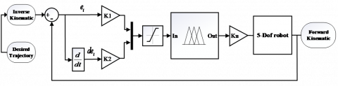
2.2.1 Structural diagram of the PD-Fuzzy controller
The control scheme for the robotic arm is illustrated in Figure 2. This controller is designed to address system uncertainties.
A fuzzy control framework for robotic applications generally includes three fundamental elements:
(i) Fuzzification: Maps the tracking error e(t) and its rate of variation de(t) into corresponding fuzzy sets through predefined membership functions.
(ii) Rule Base: Implements the Sugeno inference approach to formulate a collection of fuzzy control rules derived from expert experience.
(iii) Defuzzification: Transforms the inferred fuzzy output into a precise control signal u that is applied to the robot.
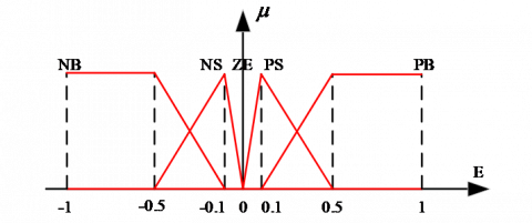
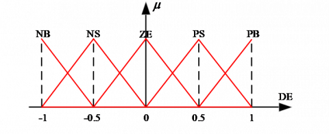
2.2.2 Membership functions
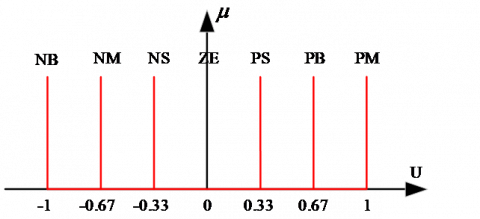
With the input variables e(t) (error), de(t) (change in error) and the output value u (control signal) defined in Figures 3-5, the linguistic variable values are constructed as follows: NB (Negative Big), NM (Negative Medium), NS (Negative Small), ZE (Zero), PS (Positive Small), PM (Positive Medium) and PB (Positive Big)
From these sets, the membership functions are constructed based on the pre-calculated PD parameters [9-11].
Figure 3. Position parameters
Figure 4. Differential position error parameters
Figure 5. Differential control signal parameters
2.2.3 Fuzzy control rules
The design of the fuzzy controller relies on expert knowledge to establish the inference rules and the defuzzification mechanism.
During the tuning process, multiple simulations were performed to observe the impact of parameter changes and to select the configuration that yields the smallest error. This iterative process helped to refine the controller, resulting in a stable fuzzy system that is well-adapted to real-world conditions.
Table 6. Fuzzy control rules for the robotic arm
|
U |
E |
|||||
|
NB |
NS |
ZE |
PS |
PB |
||
|
DE |
NB |
NB |
NB |
NM |
NS |
ZE |
|
NE |
NB |
NM |
NS |
ZE |
PS |
|
|
ZE |
NM |
NS |
ZE |
PS |
PM |
|
|
PS |
NS |
ZE |
PS |
PM |
PB |
|
|
PB |
ZE |
PS |
PM |
PB |
PB |
|
The rule base is constructed in Table 6 based on control experience and the following principles:
Originally pioneered by Kennedy and Eberhart in 1995 [12], Particle Swarm Optimization (PSO) represents a robust population-based metaheuristic inspired by the collective social dynamics observed in avian flocking or fish schooling. This stochastic search mechanism emulates the collaborative behavior of biological agents to efficiently navigate complex landscapes in pursuit of optimal solutions.
1) Objective function and tracking; performance index
To improve tracking accuracy and ensure long-term stability of the 5-DOF robotic manipulator, the Integral of Time-weighted Absolute Error (ITAE) [13] is used as the objective function in the PSO algorithm. The ITAE index is defined as follows:
$\mathrm{J}_{\mathrm{ITAE}}=\int_0^{\mathrm{T}} \mathrm{t} \cdot|\mathrm{e}(\mathrm{t})| \mathrm{dt}$ (13)
Unlike the ISE and IAE criteria, the incorporation of a time-dependent weighting factor t assigns progressively greater penalties to errors arising in the later stages of the simulation compared to those occurring during the initial transient phase. This weighting strategy guides the optimization process toward achieving a shorter settling time and enhanced asymptotic stability, thereby effectively mitigating sustained oscillations throughout trajectory tracking.
2) Simulation setup and search constraints
The search boundaries for the controller parameters were determined through preliminary simulation studies to ensure system stability and optimization efficiency. The parameter ranges were defined as follows:
$\mathrm{K}_{\mathrm{p}}, \mathrm{K}_{\mathrm{u}} \in[0,300]$ and $\mathrm{K}_{\mathrm{d}} \in[0,50]$
A narrower range was assigned to $K_d$ to avoid amplification of numerical noise, which could otherwise cause control signal chattering and instability within the 1 ms execution interval. Furthermore, constraining the overall search space reduces the likelihood of the PSO algorithm becoming trapped in local optima and improves convergence speed.
3) Particle Swarm Optimization framework
The PSO algorithm is employed to optimize the controller gains by modeling the collective behavior of a swarm. The movement of each particle i in the search space is updated at iteration t based on the velocity and position update equations. The velocity update equation is given by:
$\begin{aligned} \mathrm{v}_{\mathrm{i}, \mathrm{j}}(\mathrm{t}+\mathrm{l})= &~ \mathrm{w} \cdot \mathrm{v}_{\mathrm{i}, \mathrm{j}}(\mathrm{t})+\mathrm{c}_1 \cdot \mathrm{r}_1 \cdot\left(\text {pbest }_{\mathrm{i}, \mathrm{j}}-\mathrm{x}_{\mathrm{i}, \mathrm{j}}(\mathrm{t})\right) +\mathrm{c}_2 \cdot \mathrm{r}_2 \cdot\left(\text {gbest }_{\mathrm{j}}-\mathrm{x}_{\mathrm{i}, \mathrm{j}}(\mathrm{t})\right)\end{aligned}$ (14)
Position updating equation should be:
$\mathrm{x}_{\mathrm{i}, \mathrm{j}}(\mathrm{t}+\mathrm{l})=\mathrm{x}_{\mathrm{i}, \mathrm{j}}(\mathrm{t})+\mathrm{v}_{\mathrm{i}, \mathrm{j}}(\mathrm{t}+\mathrm{l})$ (15)
where, $v_{i, j}$ and $x_{i, j}$ represent the velocity and position of particle i in dimension j; $r_1, r_2$ are independent random numbers uniformly distributed in [0, 1]; pbest denotes the individual best position, and gbest represents the global best position discovered by the entire swarm.
The selection of PSO control parameters follows the constriction factor method to ensure the stability of the optimization process. To guarantee that the system converges without divergence, two fundamental mathematical conditions must be satisfied [12-14]:
• Sum of acceleration coefficients ($\phi$):
$\phi=\phi_1+\phi_2 \geq 4$ (16)
We set $\phi_1=\phi_2=2.05$, resulting in $\phi=4.1$, which satisfies the stability requirement.
• Constriction gain (k):
$0 \leq k \leq 1$ (17)
We selected k = 1 to maximize the convergence speed while maintaining stability.
Based on these conditions, the constriction factor $\chi$ (which determines the inertia weight w) and the acceleration coefficients (c1, c2) are calculated as:
$\chi=\frac{2 \mathrm{k}}{\left|2-\phi-\sqrt{\phi^2-4 \phi}\right|} \approx 0.7298$ (18)
Consequently, the specific numerical settings for the algorithm are:
Inertia Weight: $\mathrm{w}=\chi=0.7298$ (19)
Cognitive Coefficient: $c_1=\chi \phi_1=1.4962$ (20)
Social Coefficient: $c_2=\chi \phi_2=1.49621$ (21)
By enforcing these theoretical constraints, the PSO algorithm mitigates undesired oscillatory behavior and improves the convergence of particles toward the global optimum throughout the search process. Table 7 presents the definitive set of initialization parameters adopted in this study.
Table 7. Initialization parameters for the Particle Swarm Optimization (PSO) algorithm
|
Parameter |
Symbol |
Value |
|
Dimension |
npar |
15 |
|
Swarm Size (Number of Particles) |
npop |
50 |
|
Max Iterations |
MaxIt |
100 |
|
Inertia Weight |
w |
0.7298 |
|
Cognitive Coefficient |
c1 |
1.4962 |
|
Social Coefficient |
c2 |
1.4962 |
4) Dual-termination strategy
The PSO optimization process is governed by a dual-termination strategy to balance computational efficiency and control accuracy. In this study, the algorithm is configured with a maximum of 100 iterations. To reduce the overall simulation time, the optimization process terminates early if the Global Best Fitness ($J_{\text {gbest }}$) satisfies the following convergence criterion:
$J_{\text {qbest }} \leq \mathrm{J}_{\text {set }}$ (22)
where, Jset = 0.05 denotes the predefined performance threshold. This stopping criterion terminates the optimization process once the controller gains $\left(K_{p_i}, K_{d_i}, K_{u_i}\right)$, achieve the desired level of accuracy, thereby avoiding unnecessary computational iterations. The adoption of this mechanism substantially reduces the overall computational time and processing burden, while still ensuring that the resulting PD–Fuzzy controller preserves the required stability within the simulation environment.
After applying the PSO algorithm to optimize the PD-Fuzzy controller, we obtained a set of parameters that closely tracked the setpoint values, as shown in Table 8.
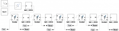
In this work, a whole simulation model for the proposed robot system is presented in Figure 6.
Together with the dynamic model shown in Figure 6, the simulation results demonstrate that the 5-DOF robotic system operates stably, with the joint movements responding well to the control signals, exhibiting smooth and precise motion. The PD-Fuzzy controller proved its effectiveness in maintaining the target trajectory.
The joint performance is illustrated in Figures 7-11.
• The system shows a fast response speed: joints 2, 3, 4 and 5 reach their reference values within the first 1–1.5 seconds. Joint 1 follows a sinusoidal trajectory, exhibiting excellent tracking performance and reaching the desired value in less than 0.5 seconds.
• The steady-state error is very small and approaches zero, as indicated by the close overlap between the blue and orange curves after the transient phase.
Table 8. Particle Swarm Optimization (PSO) parameters for searching PD-Fuzzy coefficients
|
Search Coefficient |
Value |
|
$K_{p_1}$ |
1.033e+02 |
|
$K_{d_1}$ |
1.145 |
|
$K_{u_1}$ |
1.2173e+02 |
|
$K_{p_2}$ |
2.52e+02 |
|
$K_{d_2}$ |
6.005 |
|
$K_{u_2}$ |
2.244e+02 |
|
$K_{p_3}$ |
1.045e+02 |
|
$K_{d_3}$ |
1.034 |
|
$K_{u_3}$ |
64.8099 |
|
$K_{p_4}$ |
30.156 |
|
$K_{d_4}$ |
1.046 |
|
$K_{u_4}$ |
1.155e+02 |
|
$K_{p_5}$ |
3.132 |
|
$K_{d_5}$ |
0.112 |
|
$K_{u_5}$ |
75.032 |
Figure 6. Dynamic model of the 5-DOF robot developed in Simscape – MATLAB/Simulink package

Figure 7. Comparison of Joint 1 between the reference value and the actual value
The positioning accuracy of the robot, represented by the Px and Py trajectories, is shown in Figures 12 and 13.
• It can be observed that the initial error is relatively large due to the difference between the initial position and the starting position of the robot. However, the controller rapidly drives the error to zero within the first second.
• After the transient period, the tracking error becomes extremely small, as evidenced by the close alignment of the blue curve with the orange reference curve.

Figure 8. Comparison of Joint 2 between the reference value and the actual value

Figure 9. Comparison of Joint 3 between the reference value and the actual value

Figure 10. Comparison of Joint 4 between the reference value and the actual value
To highlight the superior quality of the PD-Fuzzy controller compared to the traditional Proportional-Integral-Derivative (PID) controller, Tables 9 and 10 compare the Integral of Time-weighted Absolute Error (ITAE) and overshoot values between the two controllers.
The ITAE performance index shows significant improvement of the PD-fuzzy logic controller over the PID one.
Overshoots have been significantly reduced, demonstrating the effectiveness of the PD–Fuzzy controller smoothing the motion and reducing oscillations during start-up and stopping phases.

Figure 11. Comparison of Joint 5 between the reference value and the actual value
From the analysis results, it can be concluded that the flexible tuning of the $K_p$ and $K_d$ gains significantly contributes to maintain the stability of the robotic system.

Figure 12. Comparison of the Px parameter between the reference value and the value returned from the forward kinematics

Figure 13. Comparison of the Py parameter between the reference value and the value returned from the forward kinematics
Table 9. Comparison of ITAE values for PID and PD–Fuzzy controllers table
|
ITAE of the PD-Fuzzy Controller |
ITAE of the PID Controller |
|
0.2294 |
0.9409 |
|
0.154 |
0.4567 |
|
0.07278 |
0.2814 |
|
0.07629 |
0.7428 |
|
0.05264 |
0.195 |
Table 10. Comparison of overshoot values for PID and PD–Fuzzy controller table
|
Overshoots of the PD-Fuzzy Controller (%) |
Overshoots of the PID Controller (%) |
|
0.5005 |
1.6491 |
|
4.4711 |
17.9877 |
|
3.1025 |
5.1898 |
|
0.2871 |
79.2757 |
|
1.9845e-06 |
1.4358 |
4.1 Model training
In this study, the image processing module was implemented based on the YOLOv11 model, enabling real-time detection of multiple waste categories. It should be noted that, within the scope of this research, each image in the dataset contains only a single object.
Dataset: A large and diverse dataset is essential for developing a robust object detection model with strong generalization capability. In this study, the dataset comprises 4,664 waste images divided into five categories, specifically carton, glass, metal, paper, and plastic. The images were collected from self-captured sources and the Roboflow platform [15] to increase data variability and mitigate overfitting. Each category in the dataset exhibits distinct characteristics in terms of shape, size, color, and texture, as summarized in Tables 11 and 12, and illustrated in Figure 14.
Table 11. Number of training samples for waste classification
|
Waste Category |
Cardboard |
Glass |
Metal |
Paper |
Plastic |
|
Number of Images |
850 |
845 |
1000 |
804 |
1165 |
|
Total |
4664 |
||||
To reflect real-world operating conditions, images were collected under varied lighting conditions (natural light, strong artificial light, and low-light environments), different background types (plain white and complex backgrounds), and various camera viewpoints and distances (frontal and tilted views at multiple distances) [16-18].
During data preparation, all images were resized to 640 × 640 pixels to ensure consistency of the input data for training the YOLOv11 model. This resolution provides a balance between preserving important visual details and maintaining computational efficiency throughout the training process.
Table 12. Features of the object sample
|
Object |
Shape |
Color |
Texture |
|
Cardboard |
Box-shaped or flat sheets, potentially folded or torn. |
Light brown, gray, with printed text/labels. |
Dull surface, pressed fibers, may be wet or broken. |
|
Glass |
Bottles, jars, or fragments; cylindrical or curved shape. |
Transparent or colored (brown, white, etc.). |
Smooth, glossy and light-reflective surface. |
|
Metal |
Cans, containers, bars, or flat pieces. |
Silver, gray, or metallic sheen; may be colored. |
Hard, bright, glossy, or rusted surface. |
|
Paper |
Flat sheets, folded, crumpled or torn. |
White, brown, gray, with printed text or patterns. |
Soft, thin, wrinkled. |
|
Plastic |
Bottles, bags or containers. |
Various colors. |
Smooth or slightly rough surface, flexible/ductile. |

Figure 14. Representative samples of the five waste material categories used in the object detection dataset
To enhance the model’s generalization capability, data augmentation techniques were applied to the training set, including rotation, flipping, brightness adjustment, and contrast adjustment [19, 20]. No augmentation was applied to the validation and test sets to ensure unbiased evaluation. Subsequently, all objects were manually annotated in YOLO bounding box format using the LabelImg tool, and annotations were reviewed to ensure accuracy and consistency across all classes.
Performance metrics: To evaluate the performance of the pre-trained YOLO models, a confusion matrix was constructed at the bounding-box level for the multi-class object detection task. A predicted bounding box is considered correct if the Intersection over Union (IoU) with the corresponding ground-truth annotation is greater than or equal to 0.5. During post-processing, Non-Maximum Suppression (NMS) was applied with an IoU threshold of 0.7 to remove duplicate detections, while predictions with a confidence score below 0.25 were discarded prior to evaluation [21].
Model performance was assessed following the COCO evaluation protocol, using the metrics mAP@0.5 and mAP@0.5:0.95 [22]. Additionally, three common evaluation metrics-precision (AP), recall (AR), and F1 score (F1)-were calculated based on the model’s detection results. Mathematically, these metrics are defined as shown in Table 13.
Table 13. Structure of the confusion matrix with TP, FN, FP and TN values
|
Confusion Matrix |
Evaluation Metrics |
|||
|
|
Prediction |
Precision $=\frac{\mathrm{TP}}{\mathrm{TP}+\mathrm{FP}}$ |
||
|
Positive (P) |
Negative (N) |
Recall $=\frac{\mathrm{TP}}{\mathrm{TP}+\mathrm{FN}}$ |
||
|
Ground truth |
Positive (P) |
True Positive (TP) |
False Negative (FN) |
$\mathrm{F} 1=2 \times \frac{\text { Precision × Recall }}{\text { Precision }+ \text { Recall }}$ |
|
Negative (N) |
False Positive (FP) |
True Negative (N) |
Accuracy $=\frac{\mathrm{TP}+\mathrm{TN}}{\mathrm{TP}+\mathrm{FP}+\mathrm{TN}+\mathrm{FN}}$ |
|
The elements of the confusion matrix are defined as follows [23]:
• True Positive (TP): A correct detection where IoU ≥ 0.5 and the predicted class matches the ground-truth label.
• False Positive (FP): A detection that does not sufficiently overlap with the ground truth (IoU < 0.5) or is assigned to an incorrect class.
• True Negative (TN): Instances that do not belong to the class under consideration and are correctly not predicted as that class, following a one-vs-rest formulation.
• False Negative (FN): Objects present in the ground truth that are not detected by the model.

Figure 15. Workflow of dataset preparation for waste classification and the YOLOv11 architecture
Training: The dataset was divided into training, validation, and test sets with a ratio of 80%, 10%, and 10%, respectively. The dataset split was performed at the physical object level rather than the image level. This ensures that the same physical object does not appear in more than one subset, thereby preventing data leakage and ensuring a fair evaluation process. The dataset construction and splitting strategy ensures transparency, reproducibility, and the avoidance of data leakage, allowing reliable evaluation of the YOLOv11 model for waste detection and classification in real-world conditions.
The training workflow of the customized YOLOv11s model is illustrated in Figure 15. The training set is used to train the model, while the validation set is employed to monitor model performance during training and to support model selection or hyperparameter tuning. It can also be used to apply strategies such as early stopping. The test set is reserved for the final evaluation of the trained model.
In practice, the validation set may be derived from the training data. However, the test set must remain completely independent from both the training and validation sets to ensure that the evaluation accurately reflects the model’s generalization ability on unseen data.
The YOLOv11s model was trained using the Visual Studio Code environment. The training process utilized an NVIDIA GPU with 6 GB of memory to accelerate computation and improve training efficiency.
Table 14 below summarizes the hyperparameter values used during training of the YOLOv11s model to obtain optimal performance.
Table 14. Training hyperparameters of the YOLOv11s model
|
Hyperparameters |
Values |
|
Epochs |
30 |
|
Batch size |
12 |
|
Image size |
640 |
Simulation results: The detection performance achieved by the YOLOv11s model is presented and discussed in Figure 16.
The results shown in Figure 16 indicate that the training process of the proposed model remains stable, effective, and reliable. The YOLOv11s model shows strong learning capability, as evidenced by the continuous and consistent reduction in loss values throughout the training phase. No signs of overfitting or underfitting are observed, and the model reaches a stable and high level of performance after approximately 30 training epochs.

Figure 16. Training results of the YOLOv11s model
The first row of the training curves corresponds to the training loss components, including train/box_loss, train/cls_loss, and train/dfl_loss, all of which exhibit a smooth and monotonic decreasing trend. This trend reflects a gradual enhancement in the model’s capability to precisely localize objects (box_loss), correctly classify object categories (cls_loss), and refine the confidence distribution of bounding boxes (dfl_loss). The consistent decline observed in these loss metrics indicates that the model successfully captures representative features from the training data and steadily converges toward an optimal solution.
The second row of the training curves presents the validation loss computed on the validation dataset, including val/box_loss, val/cls_loss, and val/dfl_loss. While val/cls_loss shows relatively higher variability during the early training epochs, it progressively declines and reaches a stable pattern as the training continues. This initial fluctuation is likely associated with class imbalance in the dataset. The consistent and comparable decreasing trends observed between the training and validation loss curves suggest that the proposed model does not suffer from significant overfitting and maintains good generalization performance when evaluated on previously unseen data.
The curves associated with metrics/precision (B) and metrics/recall (B) reveal that the proposed approach maintains a robust and stable performance throughout training. Specifically, precision values rise to nearly 0.95, while recall values consistently remain around 0.90. The high precision level reflects the model’s capability to effectively suppress false positive predictions, whereas the sustained recall rate confirms its proficiency in correctly detecting target objects and minimizing missed detections.
Furthermore, the curves corresponding to mAP50 (B) and mAP50–95 (B) exhibit stable convergence at relatively high values, reaching approximately 0.96 and 0.82, respectively. The high mAP50 value reflects robust detection performance at an Intersection over Union (IoU) threshold of 0.5. The performance gap observed between mAP50 and mAP50–95 is expected, as higher IoU thresholds impose more stringent requirements on bounding box localization accuracy. Consequently, even minor deviations in predicted bounding boxes or slight inaccuracies in ground-truth annotations can lead to a noticeable reduction in the mAP50–95 metric.
As shown in Figure 17, YOLOv11 accurately identifies the label of each object.

Figure 17. Experimental results after training
Model performance on the test dataset is analyzed through a confusion matrix, which provides an overall evaluation of its capability to detect and distinguish among different waste classes. In addition, this representation facilitates the identification of class-specific misclassifications and systematic error patterns that may require further refinement.

Figure 18. Confusion matrix results of the model
The confusion matrix illustrated in Figure 18 provides an overview of the classification outcomes based on four key elements: True Positives (TP), False Positives (FP), True Negatives (TN), and False Negatives (FN). The formal definitions and detailed explanations of these elements are presented in Table 15.
As shown in Table 16, the model demonstrates strong performance in the Metal and Plastic classes, indicating effective feature extraction and robust class discrimination for these material categories.
Nevertheless, challenges persist when the model processes images containing complex backgrounds, leading to a relatively higher number of misclassifications across certain classes. In particular, a total of 182 misclassified instances is identified, with a noticeable concentration in the Cardboard and Glass categories. This pattern suggests an increased occurrence of false positive predictions in scenarios where background elements exhibit rich visual details or share similar characteristics with the target objects.
Table 15. Results from the confusion matrix
|
Components / Objects |
TP |
FP |
TN |
FN |
|
Cardboard |
680 |
71 |
3824 |
88 |
|
Glass |
847 |
156 |
3583 |
77 |
|
Metal |
976 |
110 |
3508 |
69 |
|
Paper |
610 |
42 |
3989 |
22 |
|
Plastic |
905 |
84 |
3599 |
75 |
Table 16. Evaluation of the five classes
|
Class |
Precision |
Recall |
F1-score |
|
Cardboard |
0.905 |
0.8808 |
0.8930 |
|
Glass |
0.8411 |
0.9167 |
0.8773 |
|
Metal |
0.8987 |
0.9340 |
0.9160 |
|
Paper |
0.9356 |
0.9744 |
0.9546 |
|
Plastic |
0.9207 |
0.9235 |
0.9221 |
Moreover, cross-class confusion is evident among categories with closely related visual characteristics, particularly between Cardboard and Paper, as well as Plastic and Glass. This behavior is anticipated given the similarities in color, texture, and structural appearance shared by these materials. Notably, the Cardboard and Paper classes exhibit a higher tendency toward mutual misclassification, which can be primarily attributed to their comparable material composition and surface features.
To further improve model performance, several enhancements are recommended, including the inclusion of more diverse background samples, improved class balancing within the dataset, and the application of material-specific data augmentation strategies. In addition, further fine-tuning of the model is required to strengthen its capacity to capture subtle discriminative features among visually similar categories.
Overall, the proposed model demonstrates satisfactory performance in the waste classification task, delivering stable recognition across the majority of categories. Nonetheless, further improvements in background separation, robustness to noise in real-world environments, and deeper feature representation are necessary to enhance classification accuracy. In addition, the continuous expansion and diversification of the dataset remain essential to ensure reliable performance under practical deployment conditions.
4.2 Comparative discussion
To justify the selection of YOLOv11 as the optimal model, a comparative evaluation was conducted among three YOLO variants, namely YOLOv5su, YOLOv8s, and YOLOv11. The comparison is specifically presented in Table 17 and Figure 19. They summarize the detection performance of the three YOLO models after 30 training epochs. The results indicate that YOLOv5su and YOLOv8s achieve comparable detection accuracy, whereas YOLOv11s obtains higher precision and recall values. In addition, YOLOv11s achieves the highest mAP@0.5 among the evaluated models, outperforming the two baseline approaches. These findings suggest that YOLOv11s provides improved object detection capability for the waste classification task and is well suited for integration into vision-based robotic system.
Table 18 compares the real-time performance of the evaluated YOLO models. All experiments were conducted on the same hardware platform equipped with an NVIDIA RTX3000 GPU to ensure a consistent evaluation environment. The results show that YOLOv5su achieves the highest processing speed due to its lightweight single-stage detection architecture; however, its larger model size may limit deployment on resource-constrained platforms. YOLOv8s exhibits slightly higher latency, which may be attributed to the decoupled head design that increases computational complexity during inference.
Table 17. Best performance comparison of three models after 30 training epochs
|
Model |
Best Epoch |
Precision |
Recall |
|
YOLOv5su |
28 |
0.953 |
0.786 |
|
YOLOv8s |
29 |
0.954 |
0.786 |
|
YOLOv11s |
30 |
0.957 |
0.904 |

Figure 19. Comparison of detection accuracy (mAP50) between YOLOv5su, YOLOv8su, and YOLOv11s
Table 18. Real-time performance comparison of YOLO-based models
|
Model |
Model Size (MB) |
Inference Time (ms) |
Total Latency (ms) |
FPS |
|
YOLOv5su |
14.5 |
10.5 |
14.9 |
67 |
|
YOLOv8s |
6.2 |
12.1 |
17.7 |
56 |
|
YOLOv11s |
9.4 |
12.1 |
16.0 |
62 |
In comparison, YOLOv11s achieves an inference time similar to YOLOv8s while maintaining lower overall latency and a smaller model size than YOLOv5su. These results indicate that YOLOv11s offers a balanced trade-off between detection performance, processing speed, and deployability in real-time robotic waste-sorting applications. Consequently, YOLOv11s was selected as the primary model for the robotic vision system in this study.
To evaluate the computational performance of the proposed model on embedded hardware, inference latency was measured on a Raspberry Pi 4B (ARM Cortex-A72, 4 GB RAM) using a set of 100 static test images. Each image was processed individually through the full model pipeline, and wall-clock time was recorded using Python's time.perf_counter(), capturing the duration from image input to detection output. Ten warm-up iterations were performed prior to measurement to stabilize memory allocation and remove initialization overhead. To mitigate the impact of operating system interrupts, a 5% trimmed mean was applied by excluding the five lowest and five highest latency values before computing descriptive statistics. All three models-YOLOv5su, YOLOv8s, and YOLOv11s-were evaluated under identical conditions to ensure a fair comparison.

Figure 20. Inference latency distribution of YOLOv5su, YOLOv8s, and YOLOv11s on Raspberry Pi 4B
The results, shown in Figure 20, indicate that YOLOv11s achieved an average latency of 20.3 ± 4.9 ms per frame. YOLOv8s and YOLOv5su reached 19.8 ± 7.8 ms and 19.7 ± 5.0 ms, respectively. Although the mean latency differences among the models were less than 0.6 ms-within the expected measurement noise on ARM-based hardware-a clear distinction was observed in latency stability. YOLOv11s exhibited the lowest standard deviation (4.9 ms), whereas YOLOv8s showed higher variability (7.8 ms), indicating more consistent per-frame processing. This stability is critical in practical applications such as automated waste sorting on conveyor systems, where irregular latency spikes can disrupt downstream control logic. These findings demonstrate that YOLOv11s maintains competitive inference speed on resource-constrained hardware while offering improved temporal stability compared with the baseline models.
4.3 Sending coordinates to MATLAB
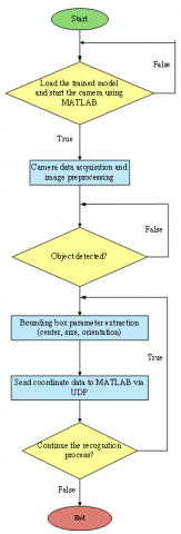
Prior to object detection and recognition by the camera system, an image preprocessing stage is performed, encompassing noise reduction, brightness enhancement and image sharpening. Subsequently, the detected objects are categorized, and their centroid positions, object counts, and orientation angles are calculated, with the results presented on the display, as illustrated in Figure 21.
Subsequently, the extracted object parameters, including positional and orientation information, are transmitted to MATLAB, where inverse kinematics calculations are carried out to determine the joint configurations required for object grasping and manipulation. The overall processing pipeline is summarized in the algorithmic flowchart shown in Figure 22.
To elucidate the operational workflow of the perception–control pipeline, the timing characteristics were quantitatively evaluated within a simulation environment. System integration was implemented using the User Datagram Protocol (UDP) to enable high-speed data exchange between the vision processing platform (Python/VSCode) and the control computation framework (MATLAB/Simulink).
1. Perception Module Timing Characteristics (Tpercept):
The image processing pipeline, based on the YOLO architecture and accelerated by GPU computation, achieves a total processing cycle of 23.3 ms. The contributions of the individual components are as follows:
+ Image Capture Time: 0.3 ms.
+ Inference Time: 22.4 ms.
+ Post-processing Time: 0.6 ms.

Figure 21. Image preprocessing
Figure 22. Flowchart of the image-processing algorithm and the position-coordinate signal transmission to MATLAB
2. Communication and Throughput Parameters (Tcomm):
The transmission of coordinate and classification data between processes is optimized for real-time responsiveness:
+ Communication Period (Comm Period): 25.9 ms.
+ Transmission Command Latency (Comm Latency): 0.1 ms.
+ System Throughput: Achieves 38.6 FPS.
+ Measured Transmission Delay: Empirical data indicates that inter-process communication latency consistently ranges between 1.27 ms and 2.76 ms.
3. Control Execution Timing (Tctrl):
In the MATLAB/Simulink environment, the control system for the 5-DOF robot is configured with the following parameters (Table 19):
+ Solver Type: ode45.
+ Maximum Step Size: Strictly set to 0.001 s (1 ms).
+ Setting the simulation step size to 1 ms provides a temporal resolution for the controller that is 25 times higher than the vision update rate, thereby contributing to the dynamic stability of the robotic manipulator during simulated operations.
Table 19. System integration and timing analysis parameters table
|
Parameter |
Value |
Unit |
|
Inference Time |
22.4 |
ms |
|
Total Software Cycle |
23.3 |
ms |
|
Communication Period |
25.9 |
ms |
|
Inter-process Latency |
1.27 - 2.76 |
ms |
|
Solver Step Size |
1.0 |
ms |
|
System Throughput |
38.6 |
Hz |
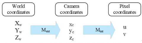
These coordinates are subsequently used as reference inputs for robot motion control. The adopted control strategy [24, 25] is implemented through two sequential stages, as illustrated in Figure 23.
Figure 23. Coordinate system transformation
Under the pinhole camera model, the mapping from three-dimensional (3D) world coordinates to the two-dimensional (2D) image plane is described by perspective projection. Based on the geometric relationship of similar triangles, the coordinates of a projected point on the image sensor, denoted as $\left(x_i, y_i\right)$, can be expressed as follows:
$x_i=f \cdot \frac{x_c}{z_c} ; y_i=f \cdot \frac{y_c}{z_c}$ (23)
where,
$x_c, y_c, z_c$: The 3D coordinates of the object in the camera coordinate system.
f: The focal length of the camera lens.
$x_i, y_i$: The 2D coordinates of the object projected onto the image plane, expressed in millimeters (mm).
To convert coordinates from the image plane (in millimeters) to the pixel coordinate plane, scaling factors $\mathrm{m}_{\mathrm{x}}$ and $\mathrm{m}_{\mathrm{y}}$ are introduced. These parameters represent the number of pixels per millimeter along the horizontal and vertical directions of the image sensor, respectively. Accordingly, the relationship between the physical focal length f and the focal lengths in pixel units, $f_x, f_y$, can be expressed as follows:
$f_x=f . m_x ; f_y=f . m_y$ (24)
The pixel coordinates (u, v) of the object are then obtained by combining the perspective projection with a translation of the coordinate origin from the image center to the top-left corner of the image frame.
$\mathrm{u}=\mathrm{f}_{\mathrm{x}} \frac{\mathrm{x}_{\mathrm{c}}}{\mathrm{z}_{\mathrm{r}}}+\mathrm{o}_{\mathrm{x}} ; \mathrm{v}=\mathrm{f}_{\mathrm{y}} \frac{\mathrm{y}_{\mathrm{c}}}{\mathrm{z}_{\mathrm{r}}}+\mathrm{o}_{\mathrm{y}}$ (25)
where, $\left(c_x, \mathrm{c}_{\mathrm{y}}\right)$ denote the principal point, which represents the offset used to shift the coordinate origin from the image center to the top-left corner of the digital image.
To represent all intrinsic parameters within a unified mathematical framework, homogeneous coordinates are employed. Under this formulation, the projection from the camera space to the pixel plane is derived from the scale equivalence between the coordinates on the virtual image plane $[\tilde{u}, \tilde{v}, \widetilde{w}]^{\mathrm{T}}$ and the corresponding pixel coordinates $[\mathrm{u}, \mathrm{v}, 1]^{\mathrm{T}}$ parameterized by the depth $\mathrm{Z}_{\mathrm{c}}$:
$\begin{aligned} {\left[\begin{array}{c}\mathrm{u} \\ \mathrm{v} \\ \mathrm{l}\end{array}\right] } & \equiv\left[\begin{array}{c}\tilde{\mathrm{u}} \\ \tilde{\mathrm{v}} \\ \widetilde{\mathrm{w}}\end{array}\right]=\left[\begin{array}{c}\mathrm{z}_{\mathrm{c}} \mathrm{u} \\ \mathrm{z}_{\mathrm{c}} \mathrm{v} \\ \mathrm{z}_{\mathrm{c}}\end{array}\right]=\left[\begin{array}{c}\mathrm{f}_{\mathrm{x}} \mathrm{x}_{\mathrm{c}}+\mathrm{z}_{\mathrm{c}} \mathrm{o}_{\mathrm{x}} \\ \mathrm{f}_{\mathrm{y}} \mathrm{y}_{\mathrm{c}}+\mathrm{z}_{\mathrm{c}} \mathrm{o}_{\mathrm{y}} \\ \mathrm{z}_{\mathrm{c}}\end{array}\right] =\left[\begin{array}{cccc}\mathrm{f}_{\mathrm{x}} & 0 & \mathrm{o}_{\mathrm{x}} & 0 \\ 0 & \mathrm{f}_{\mathrm{y}} & \mathrm{o}_{\mathrm{y}} & 0 \\ 0 & 0 & 1 & 0\end{array}\right]\left[\begin{array}{c}\mathrm{x}_{\mathrm{c}} \\ \mathrm{y}_{\mathrm{c}} \\ \mathrm{z}_{\mathrm{c}} \\ 1\end{array}\right]\end{aligned}$
Therefore,
$\tilde{\mathrm{u}}=\mathrm{M}_{\mathrm{int}} \tilde{\mathrm{x}}_{\mathrm{C}}$ (26)
where,
$u=\frac{\tilde{u}}{\widetilde{w}} ; v=\frac{\tilde{v}}{\widetilde{w}} ; M_{\text {int }}=\left[\begin{array}{ccc}f_x & 0 & o_x \\ 0 & f_y & o_y \\ 0 & 0 & 1\end{array}\right]$
The intrinsic matrix describes the internal parameters of the camera. In contrast, the extrinsic matrix Mext specifies the pose of the camera, including its translation vector t and rotation matrix R, with respect to the robot base coordinate frame.
The extrinsic matrix can be expressed as a homogeneous transformation matrix, which combines rotation and translation to transform coordinates from the world (or robot) coordinate system to the camera coordinate system:
$\left[\begin{array}{c}\mathrm{x}_{\mathrm{c}} \\ \mathrm{y}_{\mathrm{c}} \\ \mathrm{z}_{\mathrm{c}} \\ 1\end{array}\right]=\left[\begin{array}{cccc}\mathrm{r}_{11} & \mathrm{r}_{12} & \mathrm{r}_{13} & \mathrm{t}_{\mathrm{x}} \\ \mathrm{r}_{21} & \mathrm{r}_{22} & \mathrm{r}_{23} & \mathrm{t}_{\mathrm{y}} \\ \mathrm{r}_{31} & \mathrm{r}_{32} & \mathrm{r}_{33} & \mathrm{t}_{\mathrm{z}} \\ 0 & 0 & 0 & 1\end{array}\right]\left[\begin{array}{c}\mathrm{x}_{\mathrm{w}} \\ \mathrm{y}_{\mathrm{w}} \\ \mathrm{z}_{\mathrm{w}} \\ 1\end{array}\right]$
Thus,
$\tilde{\mathbf{x}}_{\mathrm{c}}=\mathrm{M}_{\mathrm{ext}} \tilde{\mathbf{x}}_{\mathrm{w}}$ (27)
where,
Rotation matrix: This is a 3 x 3 orthogonal matrix consisting of elements r11 through r33. It represents the orientation of the camera relative to the working plane.
Translation vector $\mathrm{t}\left(\mathrm{t}_{\mathrm{x}}, \mathrm{t}_{\mathrm{y}}, \mathrm{t}_{\mathrm{z}}\right)$: Comprising components tx, ty, and tz, this vector defines the position of the camera's optical center in the world space. Specifically, tz represents the operational height (working distance) from the camera lens to the object surface.
By combining Eq. (26) and Eq. (27), a transformation model from world coordinates to pixel coordinates can be obtained:
$\tilde{\mathrm{u}}=\mathrm{M}_{\text {int }} \mathrm{M}_{\mathrm{ext}} \widetilde{\mathrm{x}}_{\mathrm{W}}=\mathrm{P} \widetilde{\mathrm{x}}_{\mathrm{W}}$ (28)
Since our purpose is to determine the 3D coordinates of the object in the world and not the other way around, we used the inverse of our matrices, and the computation was realized with the following Eq. (29):
$\tilde{\mathrm{x}}_{\mathrm{w}}=\mathrm{M}_{\text {ext }}^{-1} \cdot \mathrm{M}_{\text {int }}^{-1} \cdot \tilde{\mathrm{u}}$ (29)
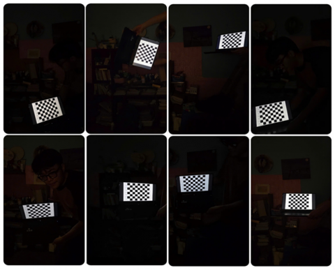
Camera calibration using the checkerboard method
To accurately determine the parameters of the intrinsic matrix $\left(\mathrm{M}_{\mathrm{int}}\right)$ and the extrinsic matrix $\left(M_{\mathrm{ext}}\right)$, the camera calibration procedure in this study follows Zhang’s method [26] based on a checkerboard pattern. This approach is widely adopted in computer vision systems due to its reliability and high calibration accuracy.
Figure 24. Experimental image dataset for camera calibration process

Figure 25. Extrinsic parameters visualization
(1) Calibration procedure
Pattern preparation: A standard checkerboard pattern with a known square size (d = 23 mm) was used as the calibration reference object (see Figure 24).
Data acquisition: The camera captured 19 images of the checkerboard pattern from different viewpoints, distances, and orientations within the robot workspace.
Image processing: The MATLAB Camera Calibrator tool was used to automatically detect the corner points of the checkerboard squares in the captured images (see Figure 25).
(2) Parameter estimation
The calibration parameters were obtained by solving an optimization problem that minimizes the reprojection error between the known corner positions on the checkerboard pattern and their corresponding pixel coordinates in the captured images. Through this process, several sets of camera parameters were extracted.
The intrinsic parameters are used to correct image distortion and ensure accurate object detection, particularly near the image boundaries. The intrinsic camera matrix is denoted as Mint.
$\begin{gathered}\mathrm{M}_{\text {int }}=\left[\begin{array}{cccc}\mathrm{f}_{\mathrm{x}} & 0 & \mathrm{o}_{\mathrm{x}} & 0 \\ 0 & \mathrm{f}_{\mathrm{y}} & \mathrm{o}_{\mathrm{y}} & 0 \\ 0 & 0 & 1 & 0\end{array}\right]= {\left[\begin{array}{cccc}2732.5 & 0 & 1978.3 & 0 \\ 0 & 2735.6 & 1506.9 & 0 \\ 0 & 0 & 1 & 0\end{array}\right]}\end{gathered}$ (30)
Radial distortion coefficients: Despite the use of the pinhole camera model, the parameters $\mathrm{k}_1$ and $\mathrm{k}_2$ are introduced to correct geometric distortions occurring toward the peripheral regions of the image, ensuring greater linearity in the projection computation.
$\mathrm{k}_1=0.0825 \pm 0.0029$
$k_2=-0.0786 \pm 0.0033$
From matrix Eq. (30) it is possible to see the intrinsic parameters as given in Table 20.
Table 20. Intrinsic parameters
|
Intrinsic Parameters |
|
|
$f_x$ |
$2732.5 \pm 7.86 p x$ |
|
$f_y$ |
$2735.6 \pm 7.95 p x$ |
|
$o_x$ |
$1978.3 \pm 2.29 p x$ |
|
$o_y$ |
$1506.9 \pm 2.29 p x$ |
Extrinsic parameters: The extrinsic parameters define the relative pose between the world coordinate system (Xw, Yw, Zw), which is attached to the checkerboard pattern, and the camera coordinate system (Xc, Yc, Zc). The extrinsic transformation matrix is denoted as (Mext).
$\begin{gathered}\mathrm{M}_{\text {ext }}=\left[\begin{array}{ll}\mathrm{R} & \mathrm{t} \\ 0 & 1\end{array}\right]=\mathrm{M}_{\text {ext }}= {\left[\begin{array}{cccc}0.9924 & -0.0249 & 0.1208 & -31.5 \\ 0.0197 & 0.9989 & 0.0435 & -490.5 \\ -0.1218 & -0.0407 & 0.9917 & 1363.4 \\ 0 & 0 & 0 & 1\end{array}\right]}\end{gathered}$ (31)
The reprojection error plot indicates that the mean calibration error is approximately 0.19 pixels. The lowest error of 0.0900054 pixels occurs in Image 5, whereas the highest error of 0.508615 pixels is observed in Figure 26.

Figure 26. Mean reprojection error per image
Using the estimated parameters $+\mathrm{f}_{\mathrm{y}} \approx 2735.6 \pm 7.95 \mathrm{px}$ và $\mathrm{t}_{\mathrm{z}} \approx 1363.4 \mathrm{~mm}$, the corresponding scale factor is calculated as follows:
$\mathrm{s}=\frac{\mathrm{t}_{\mathrm{z}}}{\mathrm{f}_{\mathrm{avg}}}=\frac{1363.4}{\frac{2732.5+2735.6}{2}} \approx 0.498\left(\frac{\mathrm{~mm}}{\mathrm{pixel}}\right)$ (32)
Using the obtained scale factor $\left(s \approx \frac{0.498 \mathrm{~mm}}{\text { pixel }}\right)$, the average 3D localization error in real-world units is computed as follows:
$\mathrm{E}_{\text {real }}=0.19 \times 0.498 \approx 0.094(\mathrm{mm})$
In terms of system implementation, it is essential to define the boundary of the present study. This research focuses on the validation of control algorithms through simulation based on CAD models integrated with a vision system prototype, rather than a full end-to-end physical robotic sorting experiment. Specifically, the robotic arm's CAD model, designed in SolidWorks, was imported into the MATLAB/Simulink environment to test the PD-Fuzzy controller's performance, yielding promising system response results. Additionally, the YOLOv11 model’s detection capability was validated using real-world image datasets and camera calibration via a checkerboard pattern. The integration of these components through the UDP protocol demonstrates the functional feasibility of the proposed system, providing a foundation for future hardware-based experiments.
In this study, a five-degree-of-freedom (5-DOF) robotic system was developed and integrated with a computer vision module to perform automated waste classification. The robotic manipulator is controlled using a PD–Fuzzy controller, which ensures precise and stable motion throughout the manipulation process. Simulation results indicate that joints 2, 3, 4, and 5 reach their reference values within approximately 1–1.5s, while maintaining a steady-state error close to zero and closely tracking the desired trajectories. Overshoot is almost negligible, demonstrating the effectiveness of the PD–Fuzzy controller in smoothing joint motions and suppressing vibrations during start-up and stopping phases. Overall, the flexible tuning of the controller gains $K_p$ and $K_d$ enables the system to maintain a high level of stability.
The perception module employs the YOLOv11 algorithm, which was trained on a dataset comprising 4,664 images across five categories of waste materials: cardboard, glass, metal, paper, and plastic. Experimental results indicate that the proposed model achieves a mean Average Precision (mAP) of 96.1%, with corresponding precision and recall values of 94.6% and 97%, respectively. These results demonstrate the model’s strong detection capability and a minimal rate of missed detections. The observed performance can be largely attributed to architectural enhancements as well as the integration of advanced training strategies.
The close integration of the vision module and the PD–Fuzzy controller enables the system to respond accurately to visual information while ensuring smooth and stable operation of the robotic arm throughout the classification process. Although the vision module still experiences certain performance degradation in complex backgrounds or between material classes with similar visual characteristics, the control simulation results confirm the crucial role of the PD–Fuzzy controller in maintaining system stability and positioning accuracy. These findings demonstrate the practical feasibility of deploying the proposed robotic system in real-world waste classification applications.
Future research will focus on expanding and diversifying the dataset, implementing material-specific data augmentation strategies, and refining feature representations to further improve classification accuracy. Additionally, further system optimization and real-world deployment studies will be conducted to assess scalability and long-term operational performance.
[1] United Nations Environment Programme. (2016). Global waste management outlook. United Nations. https://doi.org/10.18356/765baec0-en
[2] Kaza, S., Yao, L., Bhada-Tata, P., Van Woerden, F. (2018). What a waste 2.0: A global snapshot of solid waste management to 2050. World Bank Publications.
[3] Nguyen, T.D., Nakakubo, T. (2025). Characteristics of solid waste landfills in Vietnam and selection of prioritized measures based on land use-focused assessment. Journal of Material Cycles and Waste Management, 27(6): 4285-4300. https://doi.org/10.1007/s10163-025-02358-6.
[4] Tran, D.T., Nguyen, T.B.T. (2025). An intelligent plastic waste classification system based on deep learning and delta robot. Journal of Technical Education Science, 20(1): 33-42. https://doi.org/10.54644/jte.2025.1555
[5] Iliukhin, V.N., Mitkovskii, K.B., Bizyanova, D.A., Akopyan, A.A. (2017). The modeling of inverse kinematics for 5 DoF manipulator. Procedia Engineering, 176: 498-505. https://doi.org/10.1016/j.proeng.2017.02.349
[6] Chao, C.T., Teng, C.C. (1997). A PD-like self-tuning fuzzy controller without steady-state error. Fuzzy Sets and Systems, 87(2): 141-154. https://doi.org/10.1016/S0165-0114(96)00022-X
[7] Wu, H., Geng, Y., Liu, K., Liu, W. (2019). Research on programmable logic controller security. IOP Conference Series: Materials Science and Engineering, 569(4): 042031. https://doi.org/10.1051/matecconf/202440610003
[8] Pham, Q.H., Nguyen, C.H., Ly, H.N., Bui, Q.C., et al. (2025). An application of a robot arm for garbage classification using image processing and artificial intelligence. Robotica & Management, 30(1).
[9] Nguyen, N.K., Ho, S.V., Nguyen, D.T., Tran, Q.H., Tran, T.N., Nguyen, T.D. (2025). Towards an efficient control strategy for an industrial multi-DoF robotic arm. International Journal of Engineering Trends and Technology, 73(5): 328-338. https://doi.org/10.14445/22315381/IJETT-V73I5P127
[10] El-Nagar, A.M., Abdrabou, A., El-Bardini, M., Elsheikh, E.A. (2025). A class of embedded fuzzy PD controller for robot manipulator: Analytical structures and stability analysis. Soft Computing, 29(9): 4423-4448. https://doi.org/10.1007/s00500-025-10663-3
[11] Sam, V.T., Nguyen, X.H., Nguyen, N.S., Dang, H.V., Nguyen, D.H. (2024). Fuzzy PID-based trajectory control for a 5-DoF robot with disturbance compensation and Simscape integration. Journal of Measurement, Control, and Automation, 28(3): 1-8.
[12] Kennedy, J., Eberhart, R. (1995). Particle swarm optimization. Proceedings of ICNN'95-International Conference on Neural Networks, 4: 1942-1948. https://doi.org/10.1109/ICNN.1995.488968
[13] Azeez, M.I., Abdelhaleem, A.M.M., Elnaggar, S., Moustafa, K.A., Atia, K.R. (2023). Optimization of PID trajectory tracking controller for a 3-DOF robotic manipulator using enhanced Artificial Bee Colony algorithm. Scientific Reports, 13(1): 11164. https://doi.org/110.1038/s41598-023-37895-3
[14] Clerc, M., Kennedy, J. (2002). The particle swarm-explosion, stability, and convergence in a multidimensional complex space. IEEE Transactions on Evolutionary Computation, 6(1): 58-73. https://doi.org/10.1109/4235.985692
[15] Garbage Classification 3 Computer Vision Model. https://universe.roboflow.com/material-identification/garbage-classification-3.
[16] Zou, Z., Chen, K., Shi, Z., Guo, Y., Ye, J. (2023). Object detection in 20 years: A survey. Proceedings of the IEEE, 111(3): 257-276. https://doi.org/10.1109/JPROC.2023.3238524
[17] Alomar, K., Aysel, H.I., Cai, X. (2023). Data augmentation in classification and segmentation: A survey and new strategies. Journal of Imaging, 9(2): 46. https://doi.org/10.3390/jimaging9020046
[18] Hastie, T., Tibshirani, R., Friedman, J.H., Friedman, J.H. (2009). The Elements of Statistical Learning: Data Mining, Inference, and Prediction. New York: Springer.
[19] Marwah, N., Chowanda, A. (2025). A study of YOLOv11s for household waste detection: Baseline evaluation to model optimization. Procedia Computer Science, 269: 1614-1624. https://doi.org/10.1016/j.procs.2025.09.104
[20] Lin, T.Y., Maire, M., Belongie, S., Hays, J., et al. (2014). Microsoft coco: Common objects in context. In European Conference on Computer Vision, Milan, Italy, pp. 740-755. https://doi.org/10.1007/978-3-319-10602-1_48
[21] Fawcett, T. (2006). An introduction to ROC analysis. Pattern Recognition Letters, 27(8): 861-874. https://doi.org/10.1016/j.patrec.2005.10.010
[22] Davis, J., Goadrich, M. (2006). The relationship between Precision-Recall and ROC curves. In Proceedings of the 23rd International Conference on Machine Learning, Pittsburgh, USA, pp. 233-240. https://doi.org/10.1145/1143844.1143874
[23] Richardson, E., Trevizani, R., Greenbaum, J.A., Carter, H., Nielsen, M., Peters, B. (2024). The receiver operating characteristic curve accurately assesses imbalanced datasets. Patterns, 5(6): 100994. https://doi.org/10.1016/j.patter.2024.100994
[24] Hutchinson, S., Hager, G.D., Corke, P.I. (1996). A tutorial on visual servo control. IEEE Transactions on Robotics and Automation, 12(5): 651-670. https://doi.org/10.1109/70.538972
[25] Daniilidis, K. (1999). Hand-eye calibration using dual quaternions. The International Journal of Robotics Research, 18(3): 286-298. https://doi.org/10.1177/02783649922066213
[26] Zhang, Z. (2000). A flexible new technique for camera calibration. IEEE Transactions on Pattern Analysis and Machine Intelligence, 22(11): 1330-1334. https://doi.org/10.1109/34.888718