Mazin N. Ajaweed*![]() | Mazin T. Muhssin
| Mazin T. Muhssin![]() | Abbas H. Issa
| Abbas H. Issa![]() | Liana M. Cipcigan
| Liana M. Cipcigan![]()
© 2026 The authors. This article is published by IIETA and is licensed under the CC BY 4.0 license (http://creativecommons.org/licenses/by/4.0/).
OPEN ACCESS
The performance and stability of the power system significantly deteriorate due to the imbalance between electricity generation and demand. This circumstance in power systems results in frequency control challenges, referred to as frequency deviation. This paper proposes the implementation of a robust nonlinear Hybrid Optimized Sliding Mode Controller (HOSMC) and compares it with the Optimized fractional proportional-Integral-Derivative (OFPID) and Optimized Sliding Mode Controller (OSMC) for a three-area Iraqi interconnected power system to enhance the frequency response. Moreover, the parameters of the developed controllers are optimized using the Ant-Colony Optimization (ACO) technique. The proposed controllers regulate the tie-line power and frequency deviation in the analyzed three-area power system. The system will be analyzed under varying load perturbations according to the following cases: case 1: 15% uniform ramp load disturbance is applied in area 3 only at t = 8 s. Case 2 involved a step load disturbance introduced throughout three areas at different times at t = 5 s, 10 s, and 15 s, respectively. Case 3 examines white noise random with step load disturbances exclusively in area 1 only. In Case 4, the parameter uncertainties are ± 10% in synchronizing coefficients and ± 45% in the governor time constant of the gas unit. Simulation results show an improvement for settling time, peak value, and zero error steady state.
Hybrid Sliding Mode Controller, three areas, optimized fractional, proportional integral derivative, Iraqi power system, Ant-Colony Optimization
The role of electrical power distribution companies is to deliver efficient, reliable, and uninterrupted power to the consumer at an acceptable quality [1, 2]. Power systems are composed of interconnected subsystems or control areas (CAs). It is assumed that each CA consists of a coherent group of generators that are interconnected by the tie-lines. When the frequency incidence occurred at a specific area, the frequency deviates starting from that area and then propagates to other areas [3]. In modern power systems, the load frequency control (LFC) loop plays a pivotal role. It performs two essential functions: first, maintaining a constant balance between electrical generation and changes in load demand, and second, regulating power exchange between interconnected control zones, maintaining it at scheduled values. These two functions are essential for maintaining the stability and reliability of the electrical grid. In addition, the LFC loop is responsible for reducing fluctuations resulting from sudden disturbances and correcting power surpluses or shortages over a period of time that depends on the system capacity and the magnitude of the disturbance [4, 5]. Given the importance of the LFC loop, numerous control strategies have been developed to ensure its efficient performance. One of the most common and widely used approaches is the proportional-integral (PI) controller with fixed parameters. These controllers are widely used in many power systems due to their simplicity and ease of implementation [6-8]. However, this approach is not without drawbacks. PI control systems exhibit significant frequency overshoots during transient conditions and suffer from long stability periods [9]. Because of these limitations, there is a growing need for more advanced control methods. A modern controller must be able to efficiently reject disturbances, maintain consistent performance over a wide operating range, minimize transient response times without overshoots, and be flexible and able to withstand system uncertainty. Recognizing the shortcomings of conventional controllers, recent research has focused on developing new control techniques that overcome these challenges.
Below is a brief overview of the most prominent proposed approaches as presented in the recent literature. A study [10] addressed the load frequency management issue in multi-area interconnected power systems that incorporate photovoltaic and energy storage systems. Initially, a model for the solar and energy storage system is developed based on the conventional LFC framework. Subsequently, upon ascertaining the upper and lower limits of disturbances, a rapid terminal sliding mode controller is devised, which effectively mitigates the impact of disturbances. The study [11] examined LFC in a multi-area interconnected micro-grid power system, proposing a robust sliding mode control strategy utilizing an adaptive event-triggered mechanism to address frequency deviations resulting from power imbalances or time delays. A three-area power system integrated with renewable energy sources and energy storage is examined, and the relevant LFC model is constructed. Another recent study [12] proposed a decentralized LFC method for the frequency regulation of multi-area power systems utilizing an optimized integral sliding mode control (OISMC) scheme. A modified particle swarm optimization (MPSO) approach is employed to optimize the control variables of the proposed control variables of the proposed controller to enhance frequency response performance. The research [13] provides a robust controller capable of addressing oscillations in frequency regulation while maintaining simplicity. This research is presents decentralized observer sliding mode controller with H-infinity as optimization algorithm for three areas interconnected power system. The proposed controller must fulfill two objectives: robust stability and robust performance. The study [14] seeks to optimize the parameters of the LFC controller for a two-area power system comprising a reheat thermal generator and a photovoltaic (PV) power plant. An advanced multi-stage TDn (1+PI) controller is proposed to mitigate oscillations in frequency and fluctuations in tie-line power. This controller integrates a tilt-derivative with an N filter (TDn) and a PI controller, enhancing the system's response by improving both steady-state defects and the rate of change. Another study [15] proposed a fractional-order sliding mode controller for interconnected power systems with variable time delays, and performed a stability analysis using the direct Lyapunov method. Initially, a fractional Integral Sliding Mode Controller (ISMC) approach was used to enhance system stability by leveraging the flexibility of fractional systems, which contributes to widening the acceptable delay margin.
A modern study [16] presents an innovative method that integrates a continuous decentralized higher-order sliding mode controller with the honey badger algorithm (HBA), specifically tailored for LFC in multi-area power systems (MAPSs). The HBA-dHoSMO is presented to mitigate chattering and oscillations, while optimal parameters for SMC design are calculated via HBA. A modern study [17] proposes a Sliding Mode Control (SMC) technique based on a proportional integral derivative (PID) sliding surface for managing the load frequency of a standalone micro-grid power system. The main goal is to fix the frequency deviation caused by load disturbances and random power fluctuations from wind turbine generators (WTGs). The paper [18] presented a new approach to generalized sliding control based on fractional rank theory, where a fractional term is incorporated into the sliding surface to enhance the robustness of the load-frequency control system. This fractional term provides an additional degree of freedom and a wider range of tunable parameters, improving control performance. Furthermore, Markov theory is employed in the modeling process to more accurately describe parameter uncertainty and external disturbances. A modern work [19] introduces an innovative sliding mode control technique for regulating load frequency in an interconnected power system, employing a proportional-derivative sliding mode surface. The stability of the suggested system is confirmed analytically and by comparisons with classic sliding mode control and PID control schemes, demonstrating the superiority of the new approach. The authors [20] incorporate the battery energy storage model into the conventional LFC framework and offer an LFC scheme utilizing adaptive global sliding mode control to stabilize power system frequency in the presence of unanticipated load frequency deviations. An adaptive sliding mode control law is developed to dynamically modify the frequency fluctuations induced by random load disturbances. The comparing results with previous studies have been listed in Section 6.5.
The main contributions of this study are to develop a three-area model of the Iraqi power system using authentic national data, capturing the northern, central, and southern regions with a diverse mix of practical generation units including hydroelectric, gas, diesel, and thermal plants. An enhanced optimized proportional–ISMC, integrated with Ant-Colony Optimization (ACO), is designed for frequency stability analysis. The study not only strengthens Iraq’s power system but also provides a scalable framework relevant to international research on multi-area power system stability and intelligent control. This study aims to develop a Hybrid Sliding Mode Controller (HSMC) with a PI-based reaching law for multi-area LFC. Thus, an integral action is introduced in the reaching law rather than the sliding surface as usual in the ISMC approaches, improving convergence behaviour and steady-state performance. The HSMC has been improved by considering an extra switching function in addition to the traditional switching function. This adjustment seeks to diminish chattering and minimize steady-state error. The combination of these two switching functions presents a new control framework which is hereafter termed the Hybrid Optimized Sliding Mode Controller (HOSMC). This study incorporates generation source models with a dead-band constraint to control governor speed. The speed governor may not immediately react to alterations in the input signal until it reaches a specified threshold. This practical limitation has not been adequately addressed in many previous power system analyses. This work investigates nonlinear dynamics by including a saturation limiter into the governor-turbine system model for each generation source. The specified upper and lower thresholds denote the maximum and minimum power output of each generation unit.
Although the significant advances in LFC methodologies, ensuring stable frequency regulation in interconnected power systems remains challenging due to system nonlinearities, parameter uncertainties, renewable energy variability, and stochastic disturbances. Traditional sliding mode and conventional controllers offer resilience; however, they may experience steady-state errors, chattering, or constrained transient performance under significant disturbances and model uncertainties. Consequently, there is a necessity for enhanced control algorithms that can increase disturbance rejection, transient response, and robustness in multi-area power systems. This study introduces a HSMC including a PI-based reaching rule, with parameters optimally calibrated by the ACO technique. The efficacy of the suggested methodology is confirmed on a realistic three-area linked electricity system in Iraq, subjected to diverse disturbance and uncertainty situations.
This paper precisely derives three regions of the Iraqi power system based on physical data supplied by the Ministry of Electricity in Iraq. The regions of northern, central, and southern Iraq encompass different sources of power generation, including hydroelectric, gas, diesel, and thermal units. An enhanced optimized HOSMC is developed and incorporated into the model for frequency analysis. ACO has been created to enhance the controller's performance. The terms of areas have been summarized in Table 1.
Table 1. Terms used in system dynamics
|
Symbol |
Description |
Unit |
|
$x_i$ |
Area (i) state vector |
- |
|
$u_i$ |
Area (i) control input |
p.u. Mw |
|
$d_i$ |
Area (i) load disturbance |
p.u. |
|
$A_i$ |
Area (i) state matrix |
- |
|
$A_{ij}$ |
Area (i) and (j) coupling matrix |
- |
|
$B_i$ |
Input matrix |
- |
|
$F_i$ |
Disturbance matrix |
- |
|
B |
Frequency bias factor |
p.u. MW/Hz |
|
R |
Governor droop |
Hz/p.u. Mw |
|
$K_ij$ |
Tie-line coefficient |
p.u.MW/Hz |
|
$ACE_i$ |
Area Control Error for area i |
MW |
|
$∆f_i$ |
Area (i) frequency deviation |
Hz |
|
$C_o$ |
Operating capacity |
MW |
|
$C_{North}$ |
Total capacity of north |
MW |
|
$C_{central}$ |
Total capacity of central |
MW |
|
$C_{south}$ |
Total capacity of south |
MW |
|
$\text{H}_i$ |
Area inertia |
- |
|
$\text{H}_{eq}$ |
Inertia of equivalent system |
- |
|
$\text{T}_1$ |
Time constant of hydraulic governor |
Seconds |
|
$\text{T}_r$ |
Speed governor reset time constant |
Seconds |
|
$\text{T}_2$ |
Speed governor transient droop time |
Seconds |
|
$\text{T}_w$ |
Water time constant |
Seconds |
|
$\text{T}_\text{Ggas}$ |
Speed governor time constants valve position |
Seconds |
|
$\text{T}_\text{Tgas}$ |
Turbine time constant of compressor discharge |
Seconds |
|
$\text{T}_\text{Gdiesel}$ |
Diesel governor time constant |
Seconds |
|
$\text{T}_\text{Tdiesel}$ |
Diesel turbine time constant |
Seconds |
|
$\text{T}_\text{Gthermal}$ |
Thermal governor time constant |
Seconds |
|
$\text{T}_\text{Tthermal}$ |
Thermal turbine time constant |
Seconds |
|
$\text{K}_\text{pi}$ |
System model gain for area (i) |
p.u. |
|
$\text{T}_\text{pi}$ |
System model time constant for area (i) |
Seconds |
The Iraqi mathematical model of a power system presented in this research comprises three interconnected CAs, each equipped with its own load frequency controller. The linearized mathematical model for each of the three CAs can be articulated using the following Eq. (1):
$\dot{x}_i(t)=A_i x_i+\sum_{j \neq i} A_{i j} x_j+B_i u_i+F_i d_i+E_i \Delta P_i$ (1)
where, $x_i$ is the area (i) state vector, $x_j$ is a state vector of the neighbor's area, $u_i$ is the control input of area (i), $d_i$ is the disturbance load, $\Delta p_i$ is a vector of uncertainties. Matrices $A_i, A_{i j}, B_i, F_i, E_i$ represents the system matrices. The data for all regions are from the annual report of the Iraqi Ministry of Electricity for the year 2020 [21].
3.1 North area
The northern region of Iraq includes the provinces of Nineveh, Kirkuk, Salah al-Din, and Diyala, and it features a mix of power generation sources. Installed generation facilities in this area consist of hydroelectric, gas, and diesel power plants. Each facility is equipped with its own turbine and governor, whose specifications differ according to the manufacturer. Table 2 presents the operational generation capacity of this region. The equivalent system inertia $\left(\mathrm{H}_{\mathrm{eq}}\right)$ was scaled with respect to the total installed capacity and the inertia $\left(\mathrm{H}_{\mathrm{i}}\right)$ for this region was determined using Eq. (2), and its calculated value is provided in Table 2 [22].
$\mathrm{H}_{\mathrm{eq}}=\sum_{\mathrm{i}}^{\mathrm{N}} \mathrm{H}_{\mathrm{i}} \cdot \frac{\mathrm{C}_{\mathrm{o}}}{\mathrm{C}_{\mathrm{North}}}$ (2)
Table 2. Generator data and system inertia of the north region of Iraq
|
Generator Type |
Operating Capacity (MW) |
$\mathrm{H}_{\mathrm{i}}(\mathrm{s})$ |
$\mathrm{H}_{\mathrm{eq}}(\mathrm{s} \mathrm{pu})$ |
|
Hydro |
187.5 |
4.5 |
0.533688 |
|
Gas |
292 |
6 |
2.878445 |
|
Diesel |
23 |
0.945 |
0.055936 |
|
Total |
502.5 |
- |
3.468 |
3.2 Central area
The central region of Iraq encompasses the cities of Ramadi, Baghdad, Najaf, Karbala, Babil, and Diwaniyah. This region relies on a mix of power generation technologies, including hydroelectric, gas, diesel, and thermal plants. The generation units in both the northern and middle regions share the same operational parameters. The system's equivalent inertia $\left(\mathrm{H}_{\mathrm{eq}}\right)$ was normalized with respect to the total installed generation capacity. The inertia value was computed using Eq. (3) and is listed in Table 3 [22].
$H_{e q}=\sum_i^N H_i \cdot \frac{C_o}{C_{ {central }}}$ (3)
Table 3. Generator data and system inertia of the central region of Iraq
|
Generator Type |
Operating Capacity (MW) |
$\mathrm{H}_{\mathrm{i}}(\mathrm{s})$ |
$\mathrm{H}_{\mathrm{eq}}(\mathrm{s} \mathrm{pu})$ |
|
Hydro |
187.5 |
4.5 |
0.15087 |
|
Gas |
292 |
6 |
2.43004 |
|
Diesel |
23 |
0.945 |
0.04111 |
|
Thermal |
610 |
6 |
1.64709 |
|
Total |
1112.5 |
- |
4. 27 |
3.3 South area
The southern region of Iraq comprises the cities of Basra, Maysan, and Dhi Qar, and is served by a range of power generation units, including thermal, gas, and diesel plants. The same generation parameters used in the northern and middle regions were also adopted for this area. Table 4 outlines the operational generation capacity of this region. The equivalent system inertia $\left(\mathrm{H}_{\mathrm{eq}}\right)$ was normalized with respect to the total installed generation capacity. The inertia value for this region was determined using Eq. (4) and is listed in Table 4 [22].
$H_{e q}=\sum_i^N H_i \cdot \frac{C_o}{C_{ {south }}}$ (4)
Table 4. Generator data and system inertia of the south region of Iraq
|
Generator Type |
Operating Capacity (MW) |
$\mathrm{H}_{\mathrm{i}}(\mathrm{s})$ |
$\mathrm{H}_{\mathrm{eq}}(\mathrm{s} \mathrm{pu})$ |
|
Thermal |
610 |
6 |
1.51075 |
|
Gas |
292 |
6 |
2.34028 |
|
Diesel |
23 |
0.945 |
0.06868 |
|
Total |
925 |
- |
3.919 |
3.4 Iraqi interconnected model
In this research, a simplified model of an interconnected power system was developed to represent the northern, central, and southern regions of Iraq, aiming to analyze the system’s frequency response behavior, as illustrated Figure 1. The relationship between load and frequency in each region was aggregated into a damping coefficient D which was set to 1 per unit. The governor droop characteristic was modeled using the gain (1/R), assigned a value of 20 per unit across all scenarios. The parameters featured in Figure 1 are detailed in Table 5. Additionally, the frequency bias coefficient B was set to 21 per unit, as defined by Eq. (5) [22].
$B=\frac{1}{R}+D$ (5)
A multi-area power system describes regions that are linked by high-voltage transmission lines. Besides maintaining frequency stability in each region, the controller in every control area is responsible for managing power flow across the tie-lines, minimizing deviations between neighboring regions, and reducing the area control errors $\left(A C E_1, A C E_2\right.$, and $\left.A C E_3\right)$, as shown in Figure 1.
Table 5. Generators and system model parameters
|
R |
B |
T1 |
T2 |
Tr |
Tw |
TGgas |
TTgas |
TGdiesel |
TTdiesel |
TGthermal |
TTthermal |
|
0.05 |
21 |
0.2 |
38 |
5 |
1 |
0.2 |
0.3 |
0.05 |
0.2 |
0.08 |
0.3 |

Figure 1. Block diagram of the Iraqi interconnected model
The coefficient $\left(K_{i j}\right)$ equal 0.2 and denote the synchronizing torque constants between interconnected zones. The symbols ($\Delta f_1, \Delta f_2$, and $\Delta f_3$) refer to the frequency deviations in the northern, central, and southern regions, respectively. When an abrupt change in load takes place within any of the zones, the HOSMC reacts by regulating the output of the generators and reorganizing the power flow through the tie-lines allowing certain zones to export power while others import it. To ensure frequency coherence among the zones and along the interconnected paths, the area control error (ACE) must be minimized to zero promptly, while also keeping chattering effects to a minimum. The corresponding ACE formulations are provided in Eqs. (6) and (7).
$A C E_i=B_i . \Delta f_i+\sum_{j \neq i} \Delta P_{t i e, i j}$ (6)
$\Delta P_{t i e, i j}=K_{i j}\left(\Delta f_i-\Delta f_j\right)$ (7)
This section discusses the HOSMC, which is designed using the same methodology as classical sliding mode control. However, it differs by incorporating a PI term directly into the reaching laws ($u_i$), alongside the conventional switching term $\left(\tan ^{-1} \frac{S_i}{\varnothing}\right)$, in contrast to common approaches where researchers add the integral term to the sliding surface to mitigate steady-state error response.
4.1 Design of the classical Sliding Mode Control
SMC is a distinct form of variable structure control. It is recognized for its robustness, as it effectively handles model uncertainties and load-related disturbances [23-25]. The target system behavior is defined by a sliding surface $S_i(t)$, and the controller's objective is to drive the system states toward this surface and keep them there. In this work, the sliding surface $S_i(t)$ has been selected for each area; north, middle, and south, respectively as depicted in Eq. (8) below:
$S_i(t)=\lambda_{1, i} \cdot A C E_i+\lambda_{2, i} \cdot \frac{d}{d t}\left(A C E_i\right)$ (8)
where, ($\lambda_{1, \mathrm{i}} \lambda_{2, \mathrm{i}}>0$) are sliding surface weights. In this context, $A C E_1, A C E_2$, and $A C E_3$ denotes the tracking error, while ($\lambda_{1, i}, \lambda_{2, i}$) are sliding surface weights determined by the designer. The primary objective of the control strategy is to drive $A C E_1, A C E_2$, and $A C E_3$ and its derivatives to zero at all times once the sliding surfaces $S_1, S_2, S_3$ are reached. Consequently, maintaining a constant value of $S_i(t)$ requires that its time derivative be zero, which is mathematically expressed Eq. (9):
$\dot{S}_i(t)=0$ (9)
After defining the sliding surface, the control input $\mathrm{u}_{\mathrm{i}}(\mathrm{t})$ is formulated based on the conditions of the sliding mode. The sliding mode control law $\mathrm{u}_{\mathrm{i}}(\mathrm{t})$ is composed of two components: a nominal component $\mathrm{u}_{\mathrm{eq}, \mathrm{i}}(\mathrm{t})$ and a switching componentu$_{\mathrm{sw}, \mathrm{i}}(\mathrm{t})$, as described below in Eq. (10):
$u_i(t)=u_{e q, i}(t)+u_{s w, i}(t)$ (10)
where, the equivalent control term is Eq. (11):
$u_{e q, i}(t)=f(states \,\,of \,\,system)$ (11)
And for classical SMC switching term is Eq. (12):
$u_{s w, i}(t)=-k_{1 i} \cdot tan ^{-1} \frac{S_i}{\emptyset}$ (12)
And for Hybrid OSMC, the PI term is Eq. (13):
$u_{s w, i}(t)=-k_{1 i} \cdot tan ^{-1} \frac{S_i}{\emptyset}-k_{2 i} \cdot \int {sat}\left(\frac{S_i}{\emptyset}\right) \cdot d t$ (13)
The switching gains $\left(k_{1 i}, k_{2 i}>0\right)$. The model has been considered and can be written in differential form in each area. The equations from Eqs. (14)-(21) represent the north area system as follow:
$\dot{x}_1=\frac{-1}{T_{p 1}} \cdot x_1+\frac{3 K_{p 1}}{T_{p 1}} \cdot x_3+\left(-2+2 \cdot \frac{T_r}{T_2}\right) \cdot\left(\frac{K_{p 1}}{T_{p 1}}\right) \cdot x_4-\left(\frac{2 T_r}{T_2}\right) \cdot\left(\frac{K_{p 1}}{T_{p 1}}\right) \cdot x_5+\frac{K_{p 1}}{T_{p 1}} \cdot x_6+\frac{K_{p 1}}{T_{p 1}} \cdot x_8-\frac{K_{p 1}}{T_{p 1}} \cdot d i+u_i$ (14)
$\dot{x}_3=\frac{-2}{T_w} \cdot x_3+\frac{\left(\frac{2}{T_w}-2 \cdot T_r\right)}{\left(T_2 \cdot T_w\right)} \cdot x_4+\left(\frac{T_r}{T_2}\right) \cdot\left(\frac{2}{T_w}\right) \cdot \mathrm{x}_5$ (15)
$\dot{\mathrm{x}}_4=\frac{-1}{\mathrm{~T}_2} \cdot \mathrm{x}_4+\frac{1}{\mathrm{~T}_2} \cdot \mathrm{x}_5$ (16)
$\dot{\mathrm{x}}_5=\frac{-1}{\mathrm{R} \cdot \mathrm{T}_1} \cdot \mathrm{x}_1-\frac{1}{\mathrm{~T}_1} \cdot \mathrm{x}_5+\frac{1}{\mathrm{~T}_1} \cdot \mathrm{ACE}_1$ (17)
$\dot{\mathrm{x}}_6=\frac{-1}{\mathrm{~T}_{\mathrm{Ggas}}} \cdot \mathrm{x}_6+\frac{1}{\mathrm{~T}_{\mathrm{Ggas}}} \cdot \mathrm{x}_7$ (18)
$\dot{\mathrm{x}}_7=\frac{-1}{\mathrm{R} \cdot \mathrm{T}_{\mathrm{Tgas}}} \cdot \mathrm{x}_1-\frac{1}{\mathrm{~T}_{\mathrm{Tgas}}} \cdot \mathrm{x}_7+\frac{1}{\mathrm{~T}_{\mathrm{Tgas}}} \cdot \mathrm{ACE}_1$ (19)
$\dot{\mathrm{x}}_8=\frac{-1}{\mathrm{~T}_{\text {Gdiesel }}} \cdot \mathrm{x}_8+\frac{1}{\mathrm{~T}_{\text {Gdiesel }}} \cdot \mathrm{x}_9$ (20)
$\dot{\mathrm{x}}_9=\frac{-1}{\mathrm{R} \cdot \mathrm{T}_{\text {Tdiesel }}} \cdot \mathrm{x}_1-\frac{1}{\mathrm{~T}_{\text {Tdiesel }}} \cdot \mathrm{x}_9+\frac{1}{\mathrm{~T}_{\text {Tdiesel }}} \cdot \mathrm{ACE}_1$ (21)
The equations from Eqs. (22)-(31) represents the central area system as shown below:
$\dot{x}_{10}=\frac{-1}{T_{p 2}} \cdot x_{10}+\frac{3 K_{p 2}}{T_{p 2}} \cdot x_{12}+\left(-2+2 \cdot \frac{T_r}{T_2}\right) \cdot\left(\frac{K_{p 2}}{T_{p 2}}\right) \cdot x_{13}+\frac{\left(-2 \cdot T_r \cdot K_{p 2}\right)}{\left(T_2 \cdot T_{p 2}\right)} \cdot x_{14}+\frac{K_{p 2}}{T_{p 2}} \cdot x_{15}+\frac{K_{p 2}}{T_{p 2}} \cdot x_{17}+\frac{K_{p 2}}{T_{p 2}} \cdot x_{19}+u_i$ (22)
$\dot{x}_{12}=\frac{-2}{T_w} \cdot x_{12}+\left(1-\frac{T_r}{T_2}\right) \cdot\left(\frac{2}{T_w}\right) \cdot x_{13}+\left(\frac{\left(2 \cdot T_r\right)}{\left(T_2 \cdot T_w\right)}\right) \cdot x_{14}$ (23)
$\dot{x}_{13}=\frac{-1}{T_2} \cdot x_{13}+\left(\frac{1}{T_2}\right) \cdot x_{14}$ (24)
$\dot{x}_{14}=\frac{-1}{R \cdot T_1} \cdot x_{10}-\left(\frac{1}{T_1}\right) \cdot x_{14}+\left(\frac{1}{T_1}\right) \cdot A C E_2$ (25)
$\dot{x}_{15}=\frac{-1}{T_{ {Gthermal}}} \cdot x_{15}+\left(\frac{1}{T_{ {Gthermal}}}\right) \cdot x_{16}$ (26)
$\dot{x}_{16}=\frac{-1}{R \cdot T_{ {Thermal }}} \cdot x_{10}-\left(\frac{1}{T_{ {Thermal }}}\right) \cdot x_{16}+\left(\frac{1}{T_{ {Thermal }}}\right) \cdot A C E_2$ (27)
$\dot{x}_{17}=\frac{-1}{T_{G g a s}} \cdot x_{17}+\left(\frac{1}{T_{G g a s}}\right) \cdot x_{18}$ (28)
$\dot{x}_{18}=\frac{-1}{R \cdot T_{T g a s}} \cdot x_{10}-\left(\frac{1}{T_{T g a s}}\right) \cdot x_{18}+\left(\frac{1}{T_{T g a s}}\right) \cdot A C E_2$ (29)
$\dot{x}_{19}=\frac{-1}{T_{ {Gdiesel }}} \cdot x_{19}+\left(\frac{1}{T_{{Gdiesel }}}\right) \cdot x_{20}$ (30)
$\dot{x}_{20}=\frac{-1}{R \cdot T_{{Tdiesel }}} \cdot x_{10}-\left(\frac{1}{T_{ {Tdiesel }}}\right) \cdot x_{20}+\frac{1}{T_{ {Tdiesel }}} \cdot A C E_2$ (31)
The equations from Eqs. (32)-(38) represents the south area system as shown below:
$\dot{\mathrm{x}}_{21}=\frac{-1}{\mathrm{~T}_{\mathrm{p} 3}} \cdot \mathrm{x}_{21}+\left(\frac{\mathrm{K}_{\mathrm{p} 3}}{\mathrm{~T}_{\mathrm{p} 3}}\right) \cdot \mathrm{x}_{23}+\frac{\mathrm{K}_{\mathrm{p} 3}}{\mathrm{~T}_{\mathrm{p} 3}} \cdot \mathrm{x}_{25}+\frac{\mathrm{K}_{\mathrm{p} 3}}{\mathrm{~T}_{\mathrm{p} 3}} \cdot \mathrm{x}_{27}+\mathrm{u}_{\mathrm{i}}$ (32)
$\dot{\mathrm{x}}_{23}=\frac{-1}{\mathrm{T}_{\mathrm{Gthermal}}} \cdot \mathrm{x}_{23}+\left(\frac{1}{\mathrm{T}_{\mathrm{Gthermal}}}\right) \cdot \mathrm{x}_{24}$ (33)
$\dot{\mathrm{x}}_{24}=\frac{-1}{\mathrm{R} \cdot \mathrm{T}_{\text {Thermal}}} \cdot \mathrm{x}_{21}-\left(\frac{1}{\mathrm{~T}_{\text {Thermal }}}\right) \cdot \mathrm{x}_{24}+\frac{1}{\mathrm{~T}_{\text {Thermal }}} \cdot A C E_3$ (34)
$\dot{\mathrm{x}}_{25}=\frac{-1}{\mathrm{~T}_{\mathrm{Ggas}}} \cdot \mathrm{x}_{25}+\left(\frac{1}{\mathrm{~T}_{\mathrm{Ggas}}}\right) \cdot \mathrm{x}_{26}$ (35)
$\dot{\mathrm{x}}_{26}=\frac{-1}{\mathrm{R} \cdot \mathrm{T}_{\mathrm{Tgas}}} \cdot \mathrm{x}_{21}-\left(\frac{1}{\mathrm{~T}_{\mathrm{Tgas}}}\right) \cdot \mathrm{x}_{26}+\frac{1}{\mathrm{~T}_{\mathrm{Tgas}}} \cdot A C E_3$ (36)
$\dot{\mathrm{x}}_{27}=\frac{-1}{\mathrm{~T}_{\mathrm{G} \text {diesel}}} \cdot \mathrm{x}_{27}+\left(\frac{1}{\mathrm{~T}_{\mathrm{G} \text {diesel}}}\right) \cdot \mathrm{x}_{28}$ (37)
$\dot{\mathrm{x}}_{28}=\frac{-1}{\mathrm{R} \cdot \mathrm{T}_{\mathrm{Tdiesel}}} \cdot \mathrm{x}_{21}-\left(\frac{1}{\mathrm{~T}_{\mathrm{Tdiesel}}}\right) \cdot \mathrm{x}_{28}+\frac{1}{\mathrm{~T}_{\mathrm{Tdiesel}}} \cdot A C E_3$ (38)
The derivation of the sliding surface $\dot{S}_i(t)$ can be simplified for three areas; north, middle, and south after substituting the area control error $A C E_1, A C E_2$, and $A C E_3$ as follow Eqs. (39)-(41):
$\dot{\mathrm{S}}_1=\lambda_{1,1} \cdot \mathrm{~A} \dot{\mathrm{CE}}_1+\lambda_{2,1} \cdot \mathrm{~A} \ddot{\mathrm{CE}}_1$ (39)
$\dot{\mathrm{S}}_2=\lambda_{1,2} \cdot \mathrm{A} \dot{\mathrm{CE}}_2+\lambda_{2,2} \cdot \mathrm{A} \ddot{\mathrm{CE}}_2$ (40)
$\dot{\mathrm{S}}_3=\lambda_{1,3} \cdot \mathrm{A} \dot{\mathrm{CE}}_3+\lambda_{2,3} \cdot \mathrm{A} \ddot{\mathrm{CE}}_3$ (41)
To achieve Eqs. (39)-(41), the derivative of sliding surfaces $\dot{\mathrm{S}}_1, \dot{\mathrm{~S}}_2$, and $\dot{\mathrm{S}}_3$ must be reaching to zero, we substitute the differential equations of $\dot{\mathrm{x}}_1, \dot{\mathrm{x}}_{10}$, and $\dot{\mathrm{x}}_{21}$ which represent the $\Delta \mathrm{f}_1, \Delta \mathrm{f}_2$, and $\Delta \mathrm{f}_3$ respectively. After, the equations of $\mathrm{u}_{\mathrm{eq}, 1}, \mathrm{u}_{\mathrm{eq}, 2}$ and $\mathrm{u}_{\mathrm{eq}, 3}$ have been derived and presented in Eqs. (42)-(44):
$\mathrm{u}_{\mathrm{eq}, 1}=\frac{\mathrm{T}_{\mathrm{p} 1}}{\mathrm{~K}_{\mathrm{p} 1}}\left[-\lambda_{1,1} \cdot \mathrm{A} \dot{\mathrm{CE}}_1-\lambda_{2,1} \cdot \mathrm{A} \ddot{\mathrm{CE}}_1+\frac{1}{\mathrm{~T}_{\mathrm{p} 1}} \mathrm{x}_1+\frac{\mathrm{K}_{\mathrm{p} 1}}{\mathrm{~T}_{\mathrm{p} 1}} \mathrm{x}_2-\frac{3 \mathrm{~K}_{\mathrm{p} 1}}{\mathrm{~T}_{\mathrm{p} 1}} \mathrm{x}_3+\left(2-2 \frac{\mathrm{~T}_{\mathrm{r}}}{\mathrm{T}_2}\right) \cdot \frac{\mathrm{K}_{\mathrm{p} 1}}{\mathrm{~T}_{\mathrm{p} 1}} \mathrm{x}_4-\frac{2 \mathrm{~T}_{\mathrm{r}}}{\mathrm{T}_2} \cdot \frac{\mathrm{~K}_{\mathrm{p} 1}}{\mathrm{~T}_{\mathrm{p} 1}} \mathrm{x}_5-\frac{\mathrm{K}_{\mathrm{p} 1}}{\mathrm{~T}_{\mathrm{p} 1}} \mathrm{x}_6-\frac{\mathrm{K}_{\mathrm{p} 1}}{\mathrm{~T}_{\mathrm{p} 1}} \mathrm{x}_8+\frac{\mathrm{K}_{\mathrm{p} 1}}{\mathrm{~T}_{\mathrm{p} 1}} \mathrm{di}\right]$ (42)
$\mathrm{u}_{\mathrm{eq}, 2}=\frac{\mathrm{T}_{\mathrm{p} 2}}{\mathrm{~K}_{\mathrm{p} 2}}\left[-\lambda_{1,2} \cdot \mathrm{A} \dot{\mathrm{CE}}_2-\lambda_{2,2} \cdot \mathrm{A} \ddot{\mathrm{CE}}_2+\frac{1}{\mathrm{~T}_{\mathrm{p} 2}} \mathrm{x}_{10}+\frac{\mathrm{K}_{\mathrm{p} 2}}{\mathrm{~T}_{\mathrm{p} 2}} \mathrm{x}_{11}-\frac{3 \mathrm{~K}_{\mathrm{p} 2}}{\mathrm{~T}_{\mathrm{p} 2}} \mathrm{x}_{12}-\left(2-2 \frac{\mathrm{~T}_{\mathrm{r}}}{\mathrm{T}_2}\right) \cdot \frac{\mathrm{K}_{\mathrm{p} 2}}{\mathrm{~T}_{\mathrm{p} 2}} \mathrm{x}_4-\frac{2 \mathrm{~T}_{\mathrm{r}}}{\mathrm{T}_2} \cdot \frac{\mathrm{~K}_{\mathrm{p} 2}}{\mathrm{~T}_{\mathrm{p} 2}} \mathrm{x}_5-\frac{\mathrm{K}_{\mathrm{p} 2}}{\mathrm{~T}_{\mathrm{p} 2}} \mathrm{x}_6-\frac{\mathrm{K}_{\mathrm{p} 2}}{\mathrm{~T}_{\mathrm{p} 2}} \mathrm{x}_8+\frac{\mathrm{K}_{\mathrm{p} 2}}{\mathrm{~T}_{\mathrm{p} 2}} \mathrm{di}\right]$ (43)
$\mathrm{u}_{\mathrm{eq}, 3}=\frac{\mathrm{T}_{\mathrm{p} 3}}{\mathrm{~K}_{\mathrm{p} 3}}\left[-\lambda_{1,3} \cdot \mathrm{A} \dot{\mathrm{CE}}_3-\lambda_{2,3} \cdot \mathrm{A} \ddot{\mathrm{CE}}_3+\frac{1}{\mathrm{~T}_{\mathrm{p} 3}} \mathrm{x}_{21}+\frac{\mathrm{K}_{\mathrm{p} 3}}{\mathrm{~T}_{\mathrm{p} 3}} \mathrm{x}_{22}-\frac{3 \mathrm{~K}_{\mathrm{p} 3}}{\mathrm{~T}_{\mathrm{p} 3}} \mathrm{x}_3+\left(2-2 \frac{\mathrm{~T}_{\mathrm{r}}}{\mathrm{T}_2}\right) \cdot \frac{\mathrm{K}_{\mathrm{p} 3}}{\mathrm{~T}_{\mathrm{p} 3}} \mathrm{x}_4-\frac{2 \mathrm{~T}_{\mathrm{r}}}{\mathrm{T}_2} \cdot \frac{\mathrm{~K}_{\mathrm{p} 3}}{\mathrm{~T}_{\mathrm{p} 3}} \mathrm{x}_5-\frac{\mathrm{K}_{\mathrm{p} 3}}{\mathrm{~T}_{\mathrm{p} 3}} \mathrm{x}_6-\frac{\mathrm{K}_{\mathrm{p} 3}}{\mathrm{~T}_{\mathrm{p} 3}} \mathrm{x}_8+\frac{\mathrm{K}_{\mathrm{p} 3}}{\mathrm{~T}_{\mathrm{p} 3}} \mathrm{di}\right]$ (44)
Thus, the resulting sliding mode controllers ![]() for each area are presented in Eqs. (45)-(47):
for each area are presented in Eqs. (45)-(47):
$\mathrm{u}_1(\mathrm{t})=\mathrm{u}_{\mathrm{eq}, 1}-\mathrm{k}_{11} \cdot \tan ^{-1} \frac{\mathrm{~S}_1}{\emptyset}$ (45)
$\mathrm{u}_2(\mathrm{t})=\mathrm{u}_{\mathrm{eq}, 2}-\mathrm{k}_{12} \cdot \tan ^{-1} \frac{\mathrm{~S}_2}{\emptyset}$ (46)
$\mathrm{u}_3(\mathrm{t})=\mathrm{u}_{\mathrm{eq}, 3}-\mathrm{k}_{13} \cdot \tan ^{-1} \frac{\mathrm{~S}_3}{\emptyset}$ (47)
4.2 Implementation of the Hybrid Sliding Mode Controller
In this study, the HOSMC is modified by including two switching functions; conventional switching and PI switching to mitigate the chatter and the steady state error. The term $u_{s w, i}$ include the conventional switching and the PI switching is presented as Eqs. (48)-(50):
$u_1(t)=u_{e q, 1}-k_{11} \cdot tan ^{-1} \frac{S_1}{\emptyset}-k_{21} \int {sat}\left(\frac{S_1}{\emptyset}\right) \cdot d t$ (48)
$u_2(t)=u_{e q, 2}-k_{12} \cdot tan ^{-1} \frac{S_2}{\emptyset}-k_{22} \int {sat}\left(\frac{S_2}{\emptyset}\right) \cdot d t$ (49)
$u_3(t)=u_{e q, 3}-k_{13} \cdot tan ^{-1} \frac{S_3}{\emptyset}-k_{23} \int {sat}\left(\frac{S_3}{\emptyset}\right) \cdot d t$ (50)
Figure 2. Algorithmic representation of controller
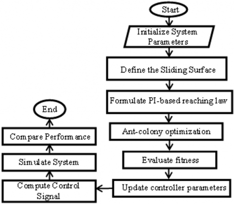
Here, $tan ^{-1} \frac{S_i}{\varnothing}$ is included in the controller to guarantee the smoothing action of the control law. The tuning parameters $\left(k_{11}, k_{21}, k_{12}, k_{22}, k_{13}\right.$, and $\left.k_{23}\right)$ are switching gains, and $(\varnothing)$ is deadband switching obtained with the use of the metaheuristic optimization techniques. The ACO technique used in this research to obtain the optimal controller parameters. The Integral Time Square Error signal (ITSE) is taken as objective function for each area as Eq. (51). The algorithmic representation of controllers are demonstrated in Figure 2.
${ITSE}=\int e(t)^2 \cdot d t$ (51)
4.3 Lyapunov stability proof
The Lyapunov assumption for each area north, central, and south as Eqs. (52)-(53):
$V_{ {area }}(t)=\frac{1}{2}\left(S_{ {area }}\right)^2$ (52)
where, $V_{ {area }}>0 \,for \,\left(S_{ {area }}(t)\right) \neq 0$, then:
$\dot{V}_{ {area }}(t)=\left(S_{ {area }}(t)\right) \cdot\left(\dot{S}_{ {area }}(t)\right)$ (53)
The proposed hybrid sliding mode control law as Eq. (54):
$u_{ {area }}=u_{ {eq,area }}+u_{ {sw,area }}$ (54)
With the hybrid switching term in Eq. (55):
$u_{ {sw,area }}=-k_{1, { area }} \cdot tan ^{-1}\left(\frac{S_{ {area }}}{\emptyset}\right)-k_{2, { area }} \cdot \int_0^t {sat}\left(\frac{S_{ {area }}}{\emptyset}\right) d t$ (55)
where, $k_{1, { area }}, k_{2, { area }}>0$, Using Eq. (8) above for each area. The sliding surface derivative for each area is given in Eq. (56):
$\dot{S}_{ {area }}=\lambda_{1, { area }} \cdot A \dot{C} E_{ {area }}+\lambda_{2, { area }} \cdot A \ddot{CE}_{ {area }}$ (56)
By choosing the equivalent control $u_{ {eq,area }}$, to eliminate the known part of the equation above, the closed loop sliding dynamics after removing known part can be written in the shorten form as Eq. (57):
$\dot{S}_{ {area }}=\varepsilon_{ {area }}(t)-k_{1, { area }} \cdot \tan ^{-1}\left(\frac{S_{ {area }}}{\emptyset}\right)-k_{2, { area }} \cdot \int_0^t {sat}\left(\frac{S_{ {area }}}{\emptyset}\right) d t$ (57)
where, $\varepsilon_{ {area }}(t)$ represents the parameter variations, load perturbations, and unmodeled dynamics that is supposed bounded as follow as Eq. (58):
$\left|\varepsilon_{ {area }}(t)\right| \leq \overline{\varepsilon_{ {area }}(t)}$ (58)
By substituting into Lyapunov derivative $\dot{V}_{ {area }}(t)$ yields as Eq. (59):
$\dot{V}_{ {area }}(t)=\left(S_{{area }}(t)\right) \cdot\left(\varepsilon_{ {area }}(t)\right)-\left(k_{1, { area }}\right) \cdot\left(S_{ {area }}(t)\right) \cdot \tan ^{-1}\left(\frac{S_{ {area }}}{\emptyset}\right)-\left(k_{2, { area }}\right) \cdot\left(S_{{area }}(t)\right) \cdot \int_0^t {sat}\left(\frac{S_{ {area }}}{\emptyset}\right) d t$ (59)
Using the inequality $\left|\left(S_{ {area }}\right) \cdot\left(\varepsilon_{ {area }}\right)\right| \leq\left(\overline{\varepsilon_{ {area }}}\right) \cdot\left|\left(S_{ {area }}\right)\right|$, so:
$\left(S_{ {area }}\right) \cdot \tan ^{-1}\left(\frac{S_{ {area }}}{\varnothing}\right)>0, \forall\left(S_{ {area }}\right) \neq 0$, we get the bound as Eq. (60):
$\dot{V}_{ {area }} \leq \overline{\varepsilon_{ {area }}} \cdot\left|\left(S_{ {area }}\right)\right| -\left(k_{1, { area }}\right) \cdot\left(S_{ {area }}(t)\right) \cdot \tan ^{-1}\left(\frac{S_{ {area }}}{\emptyset}\right)-\left(k_{2, { area}}\right) \cdot\left(S_{ {area }}(t)\right) \cdot \int_0^t {sat}\left(\frac{S_{{area }}}{\emptyset}\right) d t$ (60)
So that, by choosing the gain ($k_{1, { area}}$) to be greater than $\overline{\varepsilon_{ {area }}}$ ensures that the term $tan ^{-1}\left(\frac{S_{ {area }}}{\varnothing}\right)$ dominates the uncertainty and enforces as in Eq. (61):
$\dot{V}_{ {area }}(t)<0 \quad \forall\left(S_{ {area }}(t)\right) \neq 0$ (61)
This shows the reaching condition as Eq. (62):
$\left(S_{ {area }}(t)\right) \cdot\left(\dot{S}_{{area }}(t)\right)<0$ (62)
So, the sliding surface is attractive and the trajectories are driven toward to zero or to very close neighbourhood.
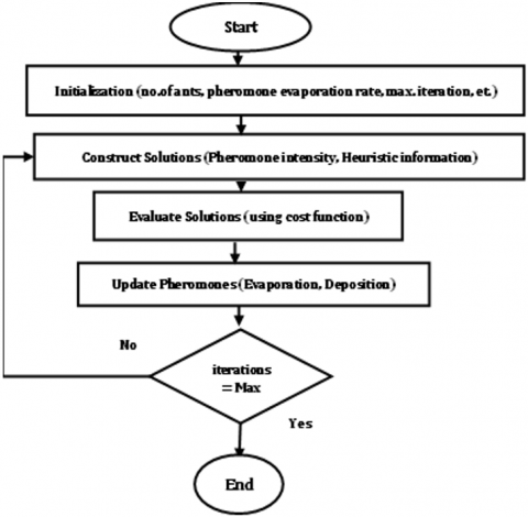
Metaheuristic optimization techniques provide efficient and economical approaches for tuning fractional controllers. These strategies depend on an objective function to evaluate solution performance and identify the optimal parameter values. ACO is a population-based metaheuristic derived on the feeding behavior of ants. Artificial ants navigate the search space and release virtual pheromones that direct subsequent solutions into favorable areas. By employing iterative pheromone update and probabilistic solution construction, ACO proficiently discovers near-optimal solutions for complicated optimization challenges. This research employs the ACO algorithm to optimize ten parameters of the HOSMC controller and fifth ten parameters of the fractional Optimized fractional proportional-Integral-Derivative (OFPID) controller, aiming to enhance system response. The cost function illustrated in Eq. (63) is used to minimize the ACE aiming for a zero error in each area by integrating the summation of the squared area control errors for three Areas ($A C E_1$), ($A C E_2$), and ($A C E_3$) multiplied by time (t).
$\text{Cost value}=\int_0^{\infty}\left(\mathrm{t} \cdot \mathrm{ACE}_1^2 \mathrm{dt}+\mathrm{t} \cdot \mathrm{ACE}_2^2 \mathrm{dt}+\mathrm{t} \cdot \mathrm{ACE}_3^2 \mathrm{dt}\right)$ (63)
In this technique, ant groups are randomly exploring the problem space for their goal. In a single zone, the controller's tuning is solely necessary to regulate the grid frequency. For an interconnected system, the controller must be tuned to fulfill various purposes, namely regulating the zonal frequency and coordinating the net exchanges across the tie-lines. To attain these objectives, a composite performance metric known as the Area Control Error (ACE) is utilized as the feedback variable in the control loop, integrating two essential components: the zonal frequency deviation (adjusted by the area's frequency bias factor) and the deviation of actual tie-line flows from their scheduled values. Consequently, lowering the ACE via the cost function can guarantee the fulfillment of both objectives as in Figure 3.
Figure 3. Ant-Colony Optimization (ACO) flowchart
This section examines a three-area interconnected power system for simulation purposes. The outcome derived from the proposed method is compared with the newly documented methods in the literature. The performance has been assessed based on peak value, settling time, and steady state error values. The simulation parameters for all cases are demonstrated in Table 6.
Table 6. Simulation parameters for all cases
|
Case Study |
Time Applied (s) |
Disturbance |
Uncertainties |
Area |
|
Case Study 1 |
8 s |
Ramp disturbance Period = 5 s |
- |
3 |
|
Case Study 2 |
5 s |
Load disturbance 15% |
- |
1 |
|
Case Study 2 |
10 s |
Load disturbance 10% |
- |
2 |
|
Case Study 2 |
15 s |
Load disturbance 15% |
- |
3 |
|
Case Study 3 |
15 s |
White noise power |
- |
1 |
|
Case Study 4 |
5 s |
Load disturbance 10% |
10% in $\left(\mathrm{K}_{12} \& \mathrm{~K}_{31}\right)$ |
1 |
|
Case Study 4 |
5 s |
Load disturbance 10% |
45% in($T_{ {Ggas }}$) |
3 |
6.1 Case study 1
This section outlines the system's testing during which it experienced a uniform ramp-type slope disturbance for a period of five seconds at t = 8seconds across area 3, as illustrated in Figures 4-6. The performance of the HOSMC is compared to that of the OSMC and the OFPID controllers in Table 7. The responses of the HOSMC demonstrate that the proposed controller exhibits lower steady-state and peak error values compared to the other controllers specifically in area3 where the disturbance has been applied. The HOSMC also achieves a smooth response with minimal chatter.

Figure 4. Frequency regulation in area 1 for case study 1

Figure 5. Frequency regulation in area 2 for case study 1

Figure 6. Frequency regulation in area 3 for case study 1
Table 7. Controllers’ response comparison for case study 1
|
Method |
Peak Value (p.u.Hz) |
Settling time (s) |
Absolute es.s |
Area |
|
OFPID |
-0.0038 |
23.38 |
0.0037 |
1 |
|
OSMC |
-0.000056 |
37.15 |
0.000043 |
1 |
|
HOSMC |
-0.00005 |
19.15 |
0.00000012 |
1 |
|
OFPID |
-0.0033 |
35.35 |
0.0037 |
2 |
|
OSMC |
-0.000062 |
50.69 |
0.000044 |
2 |
|
HOSMC |
-0.000051 |
40.32 |
0.00000014 |
2 |
|
OFPID |
-0.005 |
30.17 |
0.0038 |
3 |
|
OSMC |
-0.0015 |
20.18 |
0.0014 |
3 |
|
HOSMC |
-0.001 |
18.32 |
0.000005 |
3 |
6.2 Case study 2
This case study illustrates a severe event in which a sudden load disturbance of 15% was introduced to area 1 at t = 5 seconds, area 2 at t = 10 seconds, and area 3 at t = 15 seconds, to assess the efficacy of the proposed method via simulation in a three-area power system. Figures 7-9 display the resultant frequency deviations in areas 1, 2, and 3, as well as the power flow across the tie-line connecting the three zones during this case study. The performance of the proposed HOSMC demonstrates superior responsiveness across all three areas experiencing load disturbances at different times. Table 8 reveals lower peak and steady-state error values, accompanied by a rapid response∆.

Figure 7. Frequency regulation in area 1 for case study 2

Figure 8. Frequency regulation in area 2 for case study 2

Figure 9. Frequency regulation in area 3 for case study 2
Table 8. Controller's response comparison for case study 2
|
Method |
Peak Value (p.u.Hz) |
Settling time (s) |
Absolute es.s |
Area |
|
OFPID |
-0.005 |
33.89 |
0.004 |
1 |
|
OSMC |
-0.002 |
40.0 |
0.0005 |
1 |
|
HOSMC |
-0.001 |
19.87 |
0.0000023 |
1 |
|
OFPID |
-0.004 |
30.33 |
0.004 |
2 |
|
OSMC |
-0.001 |
21.97 |
0.0002 |
2 |
|
HOSMC |
-0.0008 |
20.85 |
0.00000013 |
2 |
|
OFPID |
-0.01 |
35.11 |
0.004 |
3 |
|
OSMC |
-0.0048 |
38.21 |
0.001 |
3 |
|
HOSMC |
-0.004 |
22.51 |
0.00000002 |
3 |
6.3 Case study 3
Following the evaluation of controller performance in response to step-load and ramp disturbances case study 3 examines the implementation of white noise power within the system. Responses of the three controllers are depicted in Figures 10-12. The data in Table 9 indicates that the proposed HOSMC outperforms competing controllers in terms of peak and steady-state error values. The settling time of HOSMC is minimized, especially in region 1, where white noise is provided.

Figure 10. Frequency regulation in area1 for case study 3

Figure 11. Frequency regulation in area 2 for case study 3

Figure 12. Frequency regulation in area 3 for case study 3
Table 9. Controller's response comparison for case study 3
|
Method |
Peak Value (p.u.Hz) |
Settling time (s) |
Absolute es.s |
Area |
|
OFPID |
-0.004 |
40.00 |
0.002 |
1 |
|
OSMC |
-0.0013 |
30.86 |
0.00032 |
1 |
|
HOSMC |
-0.0011 |
15.81 |
0.0000034 |
1 |
|
OFPID |
-0.0031 |
50.95 |
0.0026 |
2 |
|
OSMC |
-0.000065 |
40.94 |
0.000018 |
2 |
|
HOSMC |
-0.000034 |
25.87 |
0.0000014 |
2 |
|
OFPID |
-0.003 |
35.27 |
0.002 |
3 |
|
OSMC |
-0.000057 |
25.89 |
0.000013 |
3 |
|
HOSMC |
-0.00003 |
22.51 |
0.00000001 |
3 |
6.4 Case study 4
After assessing the controller, which proved effective under various abrupt load conditions, it is now being tested for scenarios involving uncertainties in the system's parameter values due to wear, damage to mechanical components, or network failures. The initial test is ±10% in $\mathrm{K}_{12}$ and $\mathrm{K}_{31}$. The second test is ±45% in $T_{ {Ggas }}$ for the area 3 governor. Figures 13-21 illustrate the controller's response. The selected uncertainty value for each parameter derives from a combination of industry practices and IEEE/IEC standard test cases. The data indicates that the proposed HOSMC demonstrates superior robustness against the uncertainties associated with $\mathrm{K}_{12}, \mathrm{~K}_{31}$, and $T_{G g a s}$, as evidenced by its minimal peak and steady-state error levels, along with the controller's smoothing behavior.

Figure 13. Frequency regulation in area1 using Hybrid Optimized Sliding Mode Controller (HOSMC) controller (K12 = ±10%)

Figure 14. Frequency regulation in area1 using Optimized Sliding Mode Controller (OSMC) controller (K12 = ± 10%)

Figure 15. Frequency regulation in area1 using Optimized fractional proportional-Integral-Derivative (OFPID) controller (K12 = ±10%)

Figure 16. Frequency regulation in area3 using Hybrid Optimized Sliding Mode Controller (HOSMC) controller (K31 = ±10%)

Figure 17. Frequency regulation in area3 using Optimized Sliding Mode Controller (OSMC) controller (K31 = ±10%)

Figure 18. Frequency regulation in area3 using Optimized fractional proportional-Integral-Derivative (OFPID)controller (K31 = ±10%)

Figure 19. Frequency regulation in area3 using Hybrid Optimized Sliding Mode Controller (HOSMC) controller (TGgas = ± 45%)

Figure 20. Frequency regulation in area3 using Optimized Sliding Mode Controller (OSMC) controller (TGgas = ± 45%)

Figure 21. Frequency regulation in area3 using Optimized fractional proportional-Integral-Derivative (OFPID) controller (TGgas = ±45%)
The results obtained from the fourth case, after exposing the system to varying percentages of uncertainty, showed that the HSMC achieved the best stability and robustness performance compared to the other traditional controllers FPID and SMC.
6.5 Comparative study with other relevant works for three areas interconnected power system
This section is carried out to provide a comprehensive comparison of our study with the literature. Table 10 includes the compared specifications. The results given in the comparative table are based on Eq. (64).
$\operatorname{improvement}(\%)=\left|\frac{\text { response (new) }- \text { response (old) }}{\text { response (new) }}\right| * 100 \%$ (64)
The comparative table illustrates the superiority of the HOSMC controller for realistic performance and robustness in managing abrupt load variations across numerous zones simultaneously. This advantage may result from constraints that introduce nonlinear characteristics to the model and controller by incorporating dead-band and saturation limitations into the generation system, which are often neglected in several research projects and consequently impact overall system performance. This performance evaluation of this study relies on comprehensive simulation models that integrate realistic system parameters, nonlinearities, and disturbance scenarios. This simulation-based analysis is commonly utilized in LFC research as an initial validation phase prior to real-time execution. However, the current study is restricted to simulation-based validation, and the real-time application of the proposed controller on hardware platforms like SCADA/PLC systems or hardware-in-the-loop testing environments represents a significant path for future investigation.
Table 10. Comparative table of numerous studies on the load frequency control (LFC)
|
Ref. |
Controller |
Saturation |
Dead Band |
Optimization |
Settling Time Improvement |
Peak Value Improvement |
Area of Load Disturbance |
|
Current study |
Hybrid Optimized Sliding Mode Controller (HOSMC) |
Included |
Included |
Ant-colony |
+76.9% |
+64.7% |
Area1 only |
|
Current study |
HOSMC |
Included |
Included |
Ant-colony |
+4.3% |
+100% |
Area2 only |
|
Current study |
HOSMC |
Included |
Included |
Ant-colony |
+65.7% |
+98.3% |
Area3 only |
|
Current study |
HOSMC |
Included |
Included |
Ant-colony |
+78.5% |
+99.5% |
All Areas |
|
[10] |
Sliding Mode Control (SMC) |
Not included |
Not included |
LMI based Lyapunov |
+50% |
+93.3% |
Area1 only |
|
[11] |
Integral Sliding Mode Controller (ISMC) |
Not included |
Not included |
Modified particle swarm optimization (MPSO) |
+16.6% |
+76% |
Area1 only |
|
[12] |
Observer SMC |
Not included |
Not included |
H-infinity |
+23% |
+78.3% |
Area1 only |
|
[12] |
Observer SMC |
Not included |
Not included |
H-infinity |
+14.3% |
+78.3% |
Area2 only |
|
[12] |
Observer SMC |
Not included |
Not included |
H-infinity |
+30% |
+78.3% |
Area3 only |
This study introduced the design of a HOSMC, Optimized Sliding Mode controller (OSMC), and Optimized Fractional (OFPID) controller for three-areas interconnected Iraqi power system. The optimal parameters for both controllers were established utilizing the ACO technique. The results from the four case studies demonstrated that the suggested HOSMC controller consistently outperformed the optimized OSMC and OFPID controller regarding settling time, peak value reduction, and steady-state error. In case study 1, the HOSMC minimized the settling time in area 1 from 23.38 seconds using OFPID and from 37.15 seconds using OSMC to 19.15 seconds and at the same time lowering the peak value from -0.0038 p.u. to -0.00005 p.u.
In case study 2, the HOSMC decreased the settling time in area 1 from 33.89 seconds to 19.87 seconds. In case study 3, the HOSMC attained the quickest stabilization, i.c., the settling time was around 15.81 seconds in area 1, in contrast to 30.86 seconds when using OSMC, while ensuring low frequency deviation across all cases.
Our forthcoming endeavors will concentrate on the development of a hybrid fractional order sliding mode controller for three-areas interconnected power system with the presence of high penetration of renewable energies such as PV, and wind turbine. Future research will examine the real-time use of the proposed controller utilizing hardware-in-the-loop platforms or SCADA/PLC settings to evaluate computational practicality.
[1] Ojha, S.K., Maddela, C.O. (2024). Load frequency control of a two-area power system with renewable energy sources using brown bear optimization technique. Electrical Engineering, 106(3): 3589-3613. https://10.1007/s00202-023-02143-4
[2] Shahzad, M.I., Gulzar, M.M., Shahzad, A., Arishi, A., Murtaza, A.F. (2026). From classical to AI-driven load frequency control: Addressing smart grid challenges with renewable energy sources and EVs integration. Renewable and Sustainable Energy Reviews, 226: 116207. https://doi.org/10.1016/j.rser.2025.116207
[3] Can, O., Ayas, M.S. (2024). Gorilla troops optimization-based load frequency control in PV-thermal power system. Neural Computing and Applications, 36(8): 4179-4193. https://doi.org/10.1007/s00521-023-09273-7
[4] Nayak, P.C., Prusty, R.C., Panda, S. (2024). Adaptive fuzzy approach for load frequency control using hybrid moth flame pattern search optimization with real time validation. Evolutionary Intelligence, 17(2): 1111-1126. https://doi.org/10.1007/s12065-022-00793-0
[5] Dhasagounder, M., Kaliannan, J., Shah, P., Sekhar, R. (2024). An Application of Artificial Bee Colony and Cohort Intelligence in the Automatic Generation Control of Thermal Power Systems. In Intelligent Methods in Electrical Power Systems, pp. 23-41.
[6] Ye, Y., Daraz, A., Basit, A., Khan, I.A., AlQahtani, S.A. (2024). Cascaded fractional-order controller-based load frequency regulation for diverse multigeneration sources incorporated with nuclear power plant. Journal of Electrical and Computer Engineering, 2024: 7939416. https://doi.org/10.1155/2024/7939416
[7] Wang, P., Chen, X., Zhang, Y., Zhang, L., Huang, Y. (2024). Fractional-order load frequency control of an interconnected power system with a hydrogen energy-storage unit. Fractal and Fractional, 8(3): 126. https://doi.org/10.3390/fractalfract8030126
[8] Dev, A., Bhatt, K., Mondal, B., Kumar, V., Kumar, V., Bajaj, M., Tuka, M.B. (2024). Enhancing load frequency control and automatic voltage regulation in Interconnected power systems using the Walrus optimization algorithm. Scientific Reports, 14(1): 27839. https://doi.org/10.1038/s41598-024-77113-2
[9] Sekyere, Y.O.M., Effah, F.B., Okyere, P.Y. (2024). Optimally tuned cascaded FOPI-FOPIDN with improved PSO for load frequency control in interconnected power systems with RES. Journal of Electrical Systems and Information Technology, 11(1): 25. https://doi.org/10.1186/s43067-024-00149-x
[10] Wang, Z., Liu, Y. (2021). Adaptive terminal sliding mode based load frequency control for multi-area interconnected power systems with PV and energy storage. IEEE Access, 9: 120185-120192. https://doi.org/10.1109/ACCESS.2021.3109141
[11] Li, H., Wang, X., Xiao, J. (2019). Adaptive event-triggered load frequency control for interconnected microgrids by observer-based sliding mode control. IEEE Access, 7: 68271-68280. https://doi.org/10.1109/ACCESS.2019.2915954
[12] Alhelou, H.H., Nagpal, N., Kassarwani, N., Siano, P. (2023). Decentralized optimized integral sliding mode-based load frequency control for interconnected multi-area power systems. IEEE Access, 11: 32296-32307. https://doi.org/10.1109/ACCESS.2023.3262790
[13] Farivar, F., Bass, O., Habibi, D. (2022). Decentralized disturbance observer-based sliding mode load frequency control in multiarea interconnected power systems. IEEE Access, 10: 92307-92320. https://doi.org/10.1109/ACCESS.2022.3201873
[14] Banu, J.B., Muthuramalingam, M., Nammalvar, P. (2022). ANFIS based double integral sliding mode control for a grid-integrated hybrid power system. Optik, 270: 170013. https://doi.org/10.1016/j.ijleo.2022.170013
[15] Yang, F., Shen, Y., Li, D., Lin, S., Muyeen, S.M., Zhai, H., Zhao, J. (2023). Fractional-order sliding mode load frequency control and stability analysis for interconnected power systems with time-varying delay. IEEE Transactions on Power Systems, 39(1): 1006-1018.https://doi.org/10.1109/TPWRS.2023.3242938
[16] Yang, F., Shao, X., Muyeen, S.M., Li, D., Lin, S., Fang, C. (2021). Disturbance observer based fractional-order integral sliding mode frequency control strategy for interconnected power system. IEEE Transactions on Power Systems, 36(6): 5922-5932. https://doi.org/10.1109/TPWRS.2021.3081737
[17] Patel, V., Guha, D., Purwar, S. (2021). Neural network aided fractional-order sliding mode controller for frequency regulation of nonlinear power systems. Computers & Electrical Engineering, 96: 107534. https://doi.org/10.1016/j.compeleceng.2021.107534
[18] Lv, X., Sun, Y., Hu, W., Dinavahi, V. (2021). Robust load frequency control for networked power system with renewable energy via fractional-order global sliding mode control. IET Renewable Power Generation, 15(5): 1046-1057. https://doi.org/10.1049/rpg2.12088
[19] Guha, D., Roy, P.K., Banerjee, S. (2023). Improved fractional-order sliding mode controller for frequency regulation of a hybrid power system with nonlinear disturbance observer. IEEE Transactions on Industry Applications, 59(4): 4964-4979. https://doi.org/10.1109/TIA.2023.3268150
[20] Huang, S., Wang, J., Xiong, L., Liu, J., Li, P., Wang, Z., Yao, G. (2021). Fixed-time backstepping fractional-order sliding mode excitation control for performance improvement of power system. IEEE Transactions on Circuits and Systems I: Regular Papers, 69(2): 956-969. https://doi.org/10.1109/TCSI.2021.3117072
[21] M. o. Electricity. (2020). Annual report of Iraqi Electricity. https://moelc.gov.iq/?page=2879.
[22] Muhssin, M T., Cipcigan, L.M., Obaid, Z.A., Al-Ansari, W.F. (2017). A novel adaptive deadbeat-based control for load frequency control of low inertia system in interconnected zones north and south of Scotland. International Journal of Electrical Power & Energy Systems, 89: 52-61. https://doi.org/10.1016/j.ijepes.2016.12.005
[23] Tawfeeq, Q.S., Al-awad, N.A., Karam, E.H. (2011). Smith predictor with simple control scheme for higher order systems. Engineering and Technology Journal, 29(3): 579-594. https://doi.org/10.30684/etj.29.3.14
[24] Hashim, S.A. (2019). Design a second order sliding mode controller for electrical servo drive systems. Engineering and Technology Journal, 37(12 Part A): 542-552. https://doi.org/10.30684/etj.37.12A.8
[25] Gorial, I. (2018). Sliding mode controller design for flexible joint robot. Engineering and Technology Journal 36(7A): 733-741. https://doi.org/10.30684/etj.36.7A.5