Van-Huy Hoang![]() | Van-Nam Pham*
| Van-Nam Pham*![]() | Thanh-Trung Nguyen
| Thanh-Trung Nguyen![]() | Thi-Hang Tran
| Thi-Hang Tran![]()
© 2026 The authors. This article is published by IIETA and is licensed under the CC BY 4.0 license (http://creativecommons.org/licenses/by/4.0/).
OPEN ACCESS
Accurate delineation of brain tumor subregions from multimodal magnetic resonance imaging (MRI) is crucial for clinical diagnosis and treatment planning; however, U-Net-based models still face difficulties in capturing long-range spatial dependencies and complex contextual variations, especially around ambiguous boundaries and irregular tumor structures. To address these challenges, we propose Residual Squeeze-and-Excitation Large Kernel Attention U-Net (ResSE-LKA-UNet), an enhanced 2D segmentation framework built upon the U-Net backbone, which integrates Residual Squeeze-and-Excitation (ResSE) blocks for channel-wise feature recalibration, Large Kernel Attention (LKA) modules to expand the receptive field and model global spatial relationships, and a Context Enhancement (CE) module to aggregate multi-scale contextual information. The proposed model is evaluated on a subset of the brain tumor segmentation (BraTS) 2021 dataset using a hybrid weighted Cross-Entropy and adaptive Tversky Dice loss under deep supervision to mitigate severe class imbalance. Qualitative analyses further confirm enhanced robustness in delineating tumors of varying sizes and morphologies, particularly in challenging edematous regions and non-enhancing tumor cores, compared with the baseline U-Net.
boundary refinement, brain tumor segmentation, U-Net, deep learning, multimodal magnetic resonance imaging
Brain tumors, particularly gliomas, remain among the most life-threatening neurological diseases due to their highly infiltrative nature, pronounced structural heterogeneity, and high recurrence rates. In parallel, the global incidence of cancer has continued to rise in recent years, posing significant challenges to healthcare systems worldwide. Accurate identification and delineation of brain tumor subregions from magnetic resonance imaging (MRI) play a pivotal role in numerous clinical applications, including surgical planning, image-guided therapeutic interventions, longitudinal tumor monitoring, and radiotherapy planning [1]. Moreover, precise tumor subregion segmentation is increasingly recognized as a fundamental prerequisite for quantitative imaging analysis, which can further contribute to prognostic assessment and overall survival prediction in patients [2].
Multimodal MRI is widely employed for brain tumor diagnosis and evaluation due to its ability to provide rich anatomical and tissue-specific information, with each imaging modality emphasizing distinct tumor characteristics such as enhancing tumor regions, necrotic cores, and peritumoral edema [3]. However, manual delineation of tumor subregions on multimodal MRI is a time-consuming and labor-intensive process that requires substantial expertise and is highly dependent on the individual experience of radiologists. In routine clinical practice, this task is predominantly performed through qualitative visual assessment, which often leads to inter-observer variability and limits its feasibility in large-scale clinical settings [4]. These limitations highlight the urgent need for automated, accurate, and reliable brain tumor segmentation (BraTS) methods that can assist clinicians, reduce workload, and improve consistency in medical image analysis. This demand for automation mirrors similar trends observed across other diagnostic domains, where deep learning-based frameworks have demonstrated strong potential in automated fault detection and predictive diagnosis from sensor signal data [5].
Early brain lesion segmentation methods mainly relied on traditional image processing techniques such as thresholding, edge detection, and clustering. For example, Sulaiman et al. [6] investigated the use of clustering-based algorithms for segmenting brain MRI images, proposing a method where an adaptive fuzzy K-means (AFKM) algorithm is used to partition the MRI intensity space and group similar tissue types, enabling automatic separation of tumor regions from healthy brain tissues. However, the performance of clustering-based methods can be sensitive to noise, the choice of initial cluster centers, and image intensity inhomogeneity, which affect the accuracy and consistency of segmentation results. While these methods could achieve reasonable performance under controlled conditions, they depended heavily on hand-crafted features and manually selected parameters, leading to a noticeable degradation in accuracy when tumor shapes became complex or MRI images were affected by noise.
With the emergence of deep learning, segmentation models began to learn feature representations automatically in an end-to-end manner. Fully Convolutional Networks (FCNs) introduced a pixel-wise segmentation framework by eliminating fully connected layers [7]; however, repeated downsampling operations often caused the loss of spatial details, resulting in blurred boundaries and limited ability to detect small tumor regions. Convolutional neural networks have since become central to medical image segmentation, among which the U-Net [8] is one of the most widely adopted architectures. Its encoder–decoder structure with skip connections effectively combines semantic context with fine-grained spatial information, making it suitable for medical tasks with limited annotated data. Building on this framework, numerous U-Net-based variants have been proposed and evaluated on the BraTS benchmark [9, 10], which has become a standard dataset for the comparative evaluation of BraTS methods.
Despite these advances, BraTS from MRI remains difficult due to several inherent factors. First, tumor subregions show large variations in appearance across different MRI modalities and across patients, leading to highly heterogeneous intensity and texture patterns. Second, tumor boundaries are often irregular and unclear, particularly in edematous regions where the transition between tumor tissue and healthy brain is gradual rather than sharp. Third, the strong imbalance between tumor and background voxels can cause models to favor the dominant background class, reducing sensitivity to small tumor regions. Finally, variations in scanners and imaging protocols across institutions introduce intensity inconsistencies that can significantly affect model robustness and generalization.
To address these challenges, recent research has focused on enhancing the representational capacity of segmentation networks. A key direction involves strengthening feature representation and recalibration. The Squeeze-and-Excitation (SE) block [11] introduced a channel-wise attention mechanism that adaptively recalibrates feature responses, showing promise in medical tasks. ResUNet incorporates residual learning into the U-Net architecture, enabling deeper feature extraction while maintaining stable gradient propagation. The use of residual blocks allows the network to effectively aggregate multi-level contextual information and enhance semantic representation, thereby improving its ability to model complex tumor structures and capture both local details and broader contextual cues [12]. The recent Large Kernel Attention (LKA) module offers an efficient decomposition of large convolutional kernels into depthwise and pointwise components, effectively modeling global context with manageable computational cost [13]. Furthermore, explicitly modeling multi-scale contextual information at the network bottleneck, where features are most abstract, can enhance semantic understanding before upsampling [14].
In this paper, we propose a novel network architecture, ResSE-LKA-UNet, designed to tackle the aforementioned limitations of existing BraTS methods. Our contributions are threefold:
2.1 Overall framework
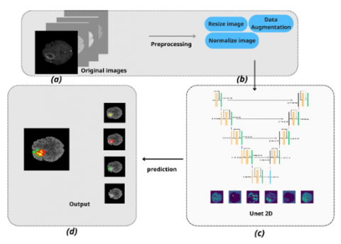
In this study, we propose an end-to-end BraTS framework based on a 2D U-Net architecture, as shown in Figure 1. The overall pipeline starts from raw 3D multi-modal MRI volumes and transforms them into 2D slices for efficient learning and inference. The framework consists of three main stages: (i) data preprocessing, (ii) tumor segmentation using an improved U-Net 2D model, and (iii) post-processing and visualization of the predicted results.
During the preprocessing stage, each 2D slice is resized to a fixed resolution, followed by intensity normalization and contrast enhancement using CLAHE. These steps help mitigate intensity inhomogeneity across different MRI scanners and improve the visibility of tumor boundaries.
The preprocessed and augmented slices are then fed into a 2D U-Net network, which adopts an encoder–decoder structure with skip connections to effectively capture both low-level spatial details and high-level semantic information. The model outputs pixel-wise segmentation masks corresponding to different tumor sub-regions.
Figure 1. Overall training framework showing: (a) Input: 4-channel magnetic resonance imaging (MRI) (T1, T1ce, T2, FLAIR), (b) Preprocessing: intensity normalization and data augmentation, (c) Proposed method, (d) Output
2.2 Proposed architecture
2.2.1 Overall architecture
In this study, we propose a BraTS model based on a 2D U-Net architecture, as shown in Figure 2, which is improved to better learn semantic features and capture spatial context in multi-modal MRI images. The proposed network keeps the symmetric encoder–decoder structure of U-Net, while incorporating Residual Squeeze-and-Excitation (ResSE), LKA, and CE modules at key stages. These improvements enhance channel-wise feature selection, enlarge the receptive field, and integrate global contextual information, thereby improving the segmentation of tumor regions with complex shapes and unclear boundaries on the BraTS 2021 dataset.
The input to the model consists of multi-modal MRI images with four channels (FLAIR, T1, T1ce, and T2), each resized to a resolution of 128 × 128. The encoder is composed of multiple resolution levels, where each level employs a Residual SE block combined with an LKA module to extract local features while enlarging the spatial receptive field. Through residual connections and channel-wise recalibration, these blocks help the network focus on tumor-related features and suppress irrelevant background noise.

Figure 2. Detailed architecture of the proposed model
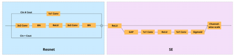
Figure 3. Residual Squeeze-and-Excitation (SE) block
At the bottleneck stage, a Context Extraction (CE) module is introduced to aggregate contextual information from multiple branches, including local features, dilated features, and global features. This design enables the model to capture long-range spatial relationships and complex tumor morphology, which is particularly beneficial for regions with diffuse edema or unclear boundaries.
The decoder progressively restores the spatial resolution through upsampling and integrates encoder features via skip connections. By leveraging the semantically enriched and selectively enhanced features from the encoder, the decoder can reconstruct more accurate segmentation maps. Finally, the output classification layer generates a multi-class segmentation map corresponding to different tumor regions in the BraTS task.
2.2.2 Residual Squeeze-and-Excitation (ResSE) block
The ResSE block is employed as a basic feature extraction unit to enhance channel-wise feature learning while maintaining the stability of deep networks. The ResSE block combines the residual architecture of ResNet with the SE mechanism [15], allowing the model to effectively capture local spatial information and automatically adjust the importance of each feature channel, as shown in Figure 3.
Given an input feature map $\mathrm{X} \in \mathbb{R}^{C \times H \times W}$, the output of the residual branch is computed as:
$\mathrm{F}=\mathrm{X}+\mathcal{R}(\mathrm{X})$ (1)
where, $\mathcal{R}(\cdot)$ denotes a sequence of $3 \times 3$, convolutional layers followed by Batch Normalization and ReLU activation.
The squeeze operation is performed using global average pooling (GAP) to obtain a channel-wise descriptor:
$z_c=\frac{1}{H \times W} \sum_{i=1}^H \sum_{j=1}^W F_c(i, j)$ (2)
Subsequently, the excitation operation generates channel attention weights through two fully connected layers and nonlinear activations, which are used to recalibrate the feature maps:
$\mathrm{s}=\sigma\left(\mathrm{W}_2 \delta\left(\mathrm{~W}_1 \mathrm{z}\right)\right), \mathrm{Y}_c=s_c \cdot F_c$ (3)
where, $\delta(\cdot)$ and $\sigma(\cdot)$ denote the ReLU and sigmoid activation functions, respectively.
The residual branch consists of two consecutive 3 × 3 convolutional layers, each followed by Batch Normalization and a ReLU activation function to extract local spatial features.
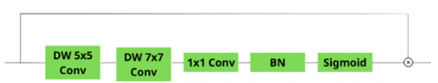
2.2.3 Large Kernel Attention module
To enhance the ability of the network to capture long-range spatial dependencies, we integrate an LKA module into the proposed segmentation framework [16]. Conventional convolutional layers with small kernel sizes are limited in modeling global contextual information [17], which is particularly important for accurately delineating complex tumor boundaries in MRI images.
The LKA module enlarges the effective receptive field by decomposing a large kernel convolution into a sequence of depthwise convolutions, allowing global spatial interactions to be modeled efficiently with a limited computational overhead. The structure of the integrated LKA module is illustrated in Figure 4.
Figure 4. Large Kernel Attention (LKA) module
As shown in Figure 4, the LKA module consists of two successive depthwise convolutions with kernel sizes of 5 × 5 and 7 × 7, followed by a 1 × 1 pointwise convolution. The depthwise convolutions are used to capture spatial information over an enlarged receptive field, while the pointwise convolution aggregates channel-wise features and refines the attention response.
Let the input feature map be denoted as:
$\mathrm{X} \in \mathbb{R}^{C \times H \times W}$ (4)
Depthwise convolutions:
$\begin{aligned} & \mathrm{F}_1=\mathrm{DWConv}_{5 \times 5}(\mathrm{X}) \\ & \mathrm{F}_2=\mathrm{DWConv}_{7 \times 7}\left(\mathrm{F}_1\right)\end{aligned}$ (5)
Pointwise convolution:
$\mathrm{F}_3=\operatorname{Conv}_{1 \times 1}\left(\mathrm{F}_2\right)$ (6)
Attention map generation:
$\mathrm{A}=\sigma\left(\mathrm{BN}\left(\mathrm{F}_3\right)\right)$ (7)
Feature recalibration:
$\mathrm{Y}=\mathrm{X} \odot \mathrm{A}$ (8)
where, $\sigma(\cdot)$ denotes the sigmoid function and $\odot$ represents element-wise multiplication.
Subsequently, batch normalization and a sigmoid activation function are applied to generate a spatial attention map. This attention map is multiplied element-wise with the input feature map, enabling the network to emphasize informative regions and suppress irrelevant background responses. Through this mechanism, the integrated LKA module improves spatial feature representation and contributes to more accurate tumor segmentation.
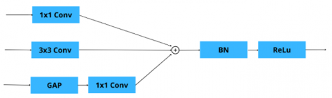
2.2.4 Context Extraction module
To enhance the representation capability of high-level semantic features, we integrate a CE module at the bottleneck of the U-Net architecture. The bottleneck layer plays a critical role in aggregating abstract semantic information after successive down-sampling operations. However, due to reduced spatial resolution, important contextual cues may be insufficiently captured when using standard convolutional operations alone.
By introducing the CE module at this stage, the network is able to jointly model local spatial details and global contextual information before feature up-sampling in the decoder. The structure of the CE module is illustrated in Figure 5.
Figure 5. Context Extraction (CE) module
As shown in Figure 5, the CE module processes the bottleneck feature map through three parallel branches. The first branch applies a 1 × 1 convolution to perform channel-wise feature transformation while preserving spatial resolution. The second branch employs a 3 × 3 convolution to capture local spatial structures and contextual patterns.
The third branch introduces global contextual awareness by applying GAP to the bottleneck feature map, followed by a 1 × 1 convolution to project the global descriptor back to the original feature space. The outputs of the three branches are fused via element-wise summation, followed by batch normalization and a ReLU activation function.
Integrating the CE module at the bottleneck allows the network to enhance high-level semantic features with complementary local and global context before they are propagated through the decoder, contributing to improved segmentation accuracy.
3.1 Datasets
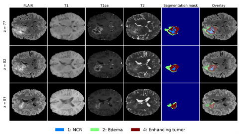
Experiments were conducted on the BraTS 2021 (2040 cases) dataset across four MRI modalities (T1, T1ce, T2, and FLAIR) [3], as illustrated in Figure 6. All experiments follow a limited-data setting. Specifically, 10% of the available cases were randomly selected using a fixed random seed of 42. These cases were first divided into training and validation sets without overlap to avoid data leakage. The selected 204 cases were split into 163 cases for training and 41 cases for validation. Preprocessing, 2D axial slice extraction, and data augmentation were then performed on the resulting splits. After training, the model was further applied to several unseen cases from the remaining data for qualitative prediction analysis. We then adopted a 5-fold cross-validation protocol.
Figure 6. Multimodal magnetic resonance imaging (MRI) visualization and tumor segmentation from (BraTS) 2021. Modalities: FLAIR, T1, T1ce, T2, ground-truth mask, and overlay. Tumor sub-regions: NCR, edema, enhancing tumor
3.2 Preprocessing
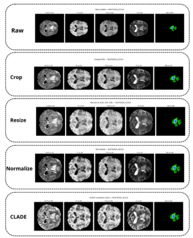
The BraTS input data are 3D multimodal MRI volumes comprising FLAIR, T1, T1ce, and T2 sequences. To reduce computational cost and memory usage, a 2D slice strategy is adopted, where axial slices are extracted from each 3D volume for segmentation. For each subject, every modality is processed independently. The images are first cropped to remove redundant background, then resized to 128 × 128. Intensity normalization is subsequently performed on the non-zero voxels of each modality volume: intensities are clipped to the [0.5th, 99.5th] percentile range and then standardized using z-score normalization. The segmentation masks are not modified, as shown in Figure 7.
Figure 7. Visualization of the preprocessing steps
For experiments using contrast enhancement, CLAHE is additionally applied to all image modalities in a slice-wise manner with a clip limit of 2.0 and a tile grid size of 8 × 8. This step is intended to improve local contrast and facilitate the delineation of subtle tumor regions and unclear boundaries.
To improve generalization under the limited-data setting, the following online augmentation transforms are applied to each training slice during loading. The augmentation transforms and corresponding parameters are summarized in Table 1.
Table 1. Data augmentation parameters used in model training
|
Augmentation |
Parameters |
|
Gaussian noise |
σ = 0.1 |
|
Additive brightness |
σ = 0.3, per-channel |
|
Gamma correction |
γ ∈ [0.7, 1.5], per-channel, retain stats |
|
Random scaling |
± 15% |
|
Random rotation |
± 15° |
|
Random cropping reflects padding |
128 × 128 (padded to 160 × 160) |
3.3 Implementation details
All experiments were conducted on a Windows 11 system equipped with an Intel Core i7-13620H processor and an NVIDIA RTX 4060 GPU with 8 GB VRAM. The proposed model was developed based on the nnUNet baseline [18], and all comparative experiments were performed under matched settings to ensure a fair comparison.
Table 2. Hardware and software configuration used in the experiments
|
Category |
Item |
Setting |
|
Optimizer |
Type |
AdamW |
|
Learning rate |
1 × 10⁻4 |
|
|
Betas |
(0.9, 0.999) |
|
|
Weight decay |
0.01 |
|
|
Epsilon |
1 × 10⁻⁵ |
|
|
Learning rate schedule |
Warmup |
Linear warmup for the first 5 epochs |
|
Decay |
Exponential decay after warmup |
|
|
Training setup |
Epochs |
50 |
|
Batch size |
8 |
|
|
Validation frequency |
Every 5 epochs |
|
|
Best model selection |
Based on the mean Dice score |
|
|
Early stopping |
Not used |
|
|
Mixed precision |
Not used |
The model was implemented in Python using the PyTorch framework and trained for 50 epochs with a batch size of 8. CUDA 12.7 and cuDNN were used to accelerate GPU computation (as detailed in Table 2).
3.4 Loss function
The proposed model is optimized using a hybrid loss function that combines weighted CE loss and an adaptive Tversky-based Dice loss, further enhanced by deep supervision at multiple decoder stages. This design aims to jointly address pixel-wise classification accuracy, region-level overlap, and training stability under severe class imbalance.
$\mathcal{L}_{\text {total }}=\sum_{i=0}^K \lambda_i \mathcal{L}_i$, (9)
where, $K=3$ denotes the number of auxiliary deep supervision outputs, $\lambda_i$ represents the weighting factor of the $i$-th output, and $\mathcal{L}_i$ is the loss computed at that output.
The deep supervision weights are empirically set as:
$\left[\lambda_0, \lambda_1, \lambda_2, \lambda_3\right]=[1.0,0.4,0.3,0.2]$ (10)
1. Weighted Cross-Entropy Loss
To perform pixel-wise multi-class classification, the weighted Cross-Entropy loss is defined as [8]:
$\mathcal{L}_{C E}=-\sum_{c=0}^{C-1} w_c y_c \log \left(\hat{p}_c\right)$ (11)
where, $C=4$ corresponds to the segmentation classes: background, ET, ED, and NCR. Here, $y_c$ denotes the one-hot encoded ground truth, and $\hat{p}_c=\operatorname{softmax}(z)_c$ represents the predicted probability for class $c$.
To mitigate the impact of class imbalance inherent in BraTS, class weights are assigned as:
$w=[0.1,1.0,1.0,1.0]$ (12)
The reduced weight for the background class prevents it from dominating the optimization process and encourages the network to focus on tumor-related regions.
2. Adaptive Tversky Dice Loss
While Cross-Entropy loss ensures discriminative pixel-wise learning, it does not explicitly optimize region overlap. Therefore, we incorporate a Dice loss based on an adaptive Tversky formulation, defined as [19]:
$\mathcal{L}_{\mathrm{T}}=1-\frac{1}{C} \sum_{c=0}^{C-1} \frac{T P_c}{T P_c+\alpha_c F P_c+\beta_c F N_c+\epsilon}$ (13)
where, $T P_c, F P_c$, and $F N_c$ denote the true positive, false positive, and false negative counts for class $c$, respectively, and $\epsilon=10^{-5}$ is a smoothing constant.
The weighting coefficients $\alpha_c$ and $\beta_c$ are adaptively determined according to the prediction error distribution:
$\alpha_c=\operatorname{clamp}\left(\frac{F P_c}{F P_c+F N_c}, 0.2,0.8\right), \beta_c=1-\alpha_c$ (14)
This adaptive mechanism dynamically balances precision and recall, which is particularly important in medical image segmentation, where false negatives are often more clinically critical than false positives.
3. Final Loss
To improve gradient propagation and accelerate convergence, deep supervision (ds) is applied at multiple decoder levels [20]. The total loss is thus expressed as:
$\mathcal{L}_{\text {total }}=\sum_{i=0}^3 \lambda_i\left(\mathcal{L}_{C E}^{(i)}+\mathcal{L}_{\mathrm{T}}^{(i)}\right)$ (15)
To be more specific:
$\mathcal{L}_{\text {total }}=1.0 \mathcal{L}_{\text {main }}+0.4 \mathcal{L}_{\mathrm{ds} 4}+0.3 \mathcal{L}_{\mathrm{ds} 3}+0.2 \mathcal{L}_{\mathrm{ds} 2}$ (16)
All auxiliary outputs are upsampled to the original resolution before loss computation. The decreasing weights reflect the progressively coarser semantic information at deeper decoder stages.
3.5 Evaluation metrics
The Dice coefficient, a statistic used to assess the similarity between the segmentation results produced by our algorithm and the ground truth labels, is calculated as:
Dice $=\frac{2 \cdot \mathrm{TP}}{\mathrm{FP}+2 \cdot \mathrm{TP}+\mathrm{FN}}$ (17)
where, TP denotes true positives, FP false positives, and FN false negatives.
The 95th percentile Hausdorff distance (HD95) quantifies the spatial discrepancy between the segmented tumor and the ground truth. It is defined as:
HD95 $=H_D(X, Y)=\max \left(d_{x y}, d_{y x}\right)$ (18)
where, $d_{x y}$ and $d_{y x}$ represent the 95th percentile of the distances from points in set X to their nearest neighbors in set Y , and vice versa. A lower HD95 value signifies a closer spatial agreement between the predicted and actual tumor boundaries.
4.1 Quantitative results
The proposed model was evaluated on the BraTS dataset using 5-fold cross-validation. Segmentation performance was assessed using two widely adopted metrics: DSC and HD95. These metrics were computed for three clinically relevant tumor subregions, namely the enhancing tumor (ET), edema (ED), and necrotic and non-enhancing tumor core (NCR). The mean and standard deviation of each metric are reported in Table 3.
Table 3. Quantitative segmentation performance on the dataset
|
Fold |
DSC (%) |
HD95 (mm) |
||||
|
NCR |
ET |
ED |
NCR |
ET |
ED |
|
|
1 |
82.10 |
79.40 |
74.20 |
2.40 |
4.20 |
5.10 |
|
2 |
90.30 |
86.50 |
84.60 |
5.80 |
7.10 |
9.20 |
|
3 |
85.60 |
83.10 |
78.30 |
3.90 |
5.90 |
6.80 |
|
4 |
81.70 |
78.60 |
73.90 |
5.20 |
6.40 |
8.50 |
|
5 |
88.90 |
85.20 |
82.10 |
4.60 |
6.80 |
7.90 |
|
Mean |
85.72 |
82.56 |
78.62 |
4.38 |
6.08 |
7.50 |
|
Std Dev |
3.81 |
3.53 |
4.58 |
1.34 |
1.11 |
1.62 |
The proposed model achieves average Dice scores of 85.72%, 82.56%, and 78.62% for the NCR, ET, and ED subregions, respectively, indicating accurate region-wise segmentation across different tumor components. In terms of boundary accuracy, the corresponding mean HD95 values are 4.38 mm (NCR), 6.08 mm (ET), and 7.50 mm (ED). The relatively low standard deviations across all folds demonstrate the robustness and stability of the proposed method under different data splits, while the slightly lower performance on ED reflects the inherent difficulty of segmenting diffuse tumor regions.
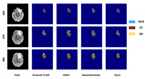
Qualitative comparisons were conducted on representative BraTS cases with small and large tumor sizes. These examples were selected to visually illustrate the model’s behavior across varying lesion extents and structural complexities. Visualization results are provided in Figures 8 and 9.
Figure 8. Segmentation results on the brain tumor segmentation (BraTS) dataset for tumors of large sizes
Table 4. Dice score comparison (%) for large tumors corresponding to Figure 8
|
Sample |
Method |
NCR/NET |
Edema (ED) |
Enhancing Tumor (ET) |
|
060 |
U-Net |
0.9211 |
0.3000 |
0.9221 |
|
Attention U-Net |
0.8717 |
0.3229 |
0.9053 |
|
|
Ours |
0.9443 |
0.3265 |
0.9527 |
|
|
070 |
U-Net |
0.9704 |
0.6258 |
0.9471 |
|
Attention U-Net |
0.9442 |
0.6313 |
0.9384 |
|
|
Ours |
0.9671 |
0.7707 |
0.9466 |
|
|
080 |
U-Net |
0.9635 |
0.7539 |
0.9656 |
|
Attention U-Net |
0.9140 |
0.7386 |
0.9391 |
|
|
Ours |
0.9515 |
0.7812 |
0.9516 |
Table 4 demonstrates that the proposed model achieves stable performance on large tumor cases, particularly in the segmentation of the NCR/NET and enhancing tumor (ET) regions. Notably, the accuracy in delineating the edema (ED) region shows a clear improvement compared to the other two models. This subregion often exhibits blurred boundaries and a diffuse appearance, making it challenging for baseline architectures such as U-Net and Attention U-Net to segment accurately. Owing to its multi-scale feature extraction capability and enhanced spatial representation, our method enables more precise identification of ED areas with unclear margins, while maintaining consistent separation of tumor substructures. The higher Dice scores across most samples confirm the effectiveness and reliability of the proposed model in handling large and complex lesions.
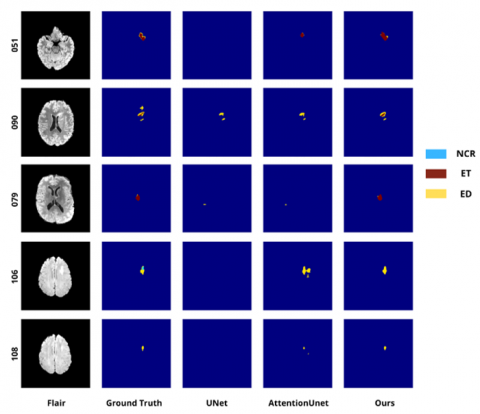
Table 5 shows that small-tumor segmentation remains a major challenge for baseline models, as these lesions occupy only a very limited area and often present ambiguous boundaries. In many cases, U-Net fails to generate meaningful predictions, as evidenced by Dice scores of 0 for the edema (ED) and enhancing tumor (ET) regions. Although Attention U-Net provides a slight improvement, its performance remains unstable and it still tends to miss tumor regions that are very small or weakly visible. In this table, “–” indicates that the corresponding class is not present in the ground-truth (GT) annotation; therefore, the metric is not applicable for that case.
Figure 9. Segmentation results on the brain tumor segmentation (BraTS) dataset for tumors of small sizes
Table 5. Dice score comparison (%) for small tumors corresponding to Figure 9
|
Sample |
Model |
NCR/NET |
Edema |
Enhancing |
|
051 |
UNet |
- |
0.0000 |
0.0000 |
|
AttUNet |
- |
0.1714 |
0.5831 |
|
|
Ours |
- |
0.1575 |
0.8012 |
|
|
090 |
UNet |
- |
0.4920 |
0.0000 |
|
AttUNet |
- |
0.5055 |
0.1159 |
|
|
Ours |
- |
0.5900 |
0.7591 |
|
|
079 |
UNet |
- |
0.0000 |
0.0000 |
|
AttUNet |
- |
0.0000 |
0.0000 |
|
|
Ours |
- |
0.0000 |
0.9017 |
|
|
106 |
UNet |
0.0000 |
0.0000 |
- |
|
AttUNet |
0.0000 |
0.5135 |
- |
|
|
Ours |
0.0000 |
0.7808 |
- |
|
|
108 |
UNet |
- |
0.0000 |
- |
|
AttUNet |
- |
0.5271 |
- |
|
|
Ours |
- |
0.8606 |
- |
In contrast, the proposed model achieves better performance and shows higher sensitivity in detecting small lesions, especially in the ET region, which is important for assessing tumor malignancy. In addition, the clear improvement in the ED region suggests that our method can better capture diffuse tumor patterns even when the lesion appears at a very small scale. These results confirm the effectiveness and reliability of the proposed model in difficult cases, where traditional approaches often fail or provide incomplete predictions.
In this study, we proposed a novel segmentation framework for brain tumor subregion delineation on the BraTS 2021 dataset. The proposed model was designed to improve the representation of tumor structures by combining multi-scale feature extraction and enhanced spatial learning. Experimental results demonstrate that our approach achieves more stable and accurate performance compared to baseline methods such as U-Net and Attention U-Net.
In particular, the proposed model shows clear improvements in challenging tumor regions, especially edema (ED), which often presents blurred boundaries and diffuse patterns. Moreover, the model is able to better detect small lesions, where traditional architectures frequently fail to produce valid predictions. Both quantitative results and qualitative comparisons confirm the reliability and robustness of our method across different tumor sizes and complex cases.
Although the proposed method achieves promising results, several directions can be explored in future research. First, we plan to evaluate the model on larger datasets and additional multi-center MRI benchmarks to further validate its generalization ability. Second, incorporating transformer-based attention mechanisms or more advanced feature fusion strategies may further enhance segmentation accuracy, especially in extremely small or heterogeneous tumor regions.
In addition, future work could investigate semi-supervised or weakly supervised learning approaches to reduce the dependence on fully annotated data, which is often limited in medical imaging. Finally, optimizing the computational efficiency of the model will also be an important step toward real-time clinical deployment.
This work was supported by the Project Granted number [49-2024-RD/HĐ – ĐHCN], Hanoi University of Industry.
[1] Martens, C., Rovai, A., Bonatto, D., Metens, T., Debeir, O., Decaestecker, C., Goldman, S., Van Simaeys, G. (2022). Deep learning for reaction-diffusion glioma growth modeling: Towards a fully personalized model?. Cancers, 14(10): 2530. https://doi.org/10.3390/cancers14102530
[2] Rastogi, D., Johri, P., Donelli, M., Kadry, S., Khan, A.A., Espa, G., Feraco, P., Kim, J. (2025). Deep learning-integrated MRI brain tumor analysis: Feature extraction, segmentation, and Survival Prediction using Replicator and volumetric networks. Scientific Reports, 15(1): 1437. https://doi.org/10.1038/s41598-024-84386-0
[3] Baid, U., Ghodasara, S., Mohan, S., Bilello, M., et al. (2021). The RSNA-ASNR-MICCAI BraTS 2021 benchmark on brain tumor segmentation and radiogenomic classification. arXiv preprint arXiv:2107.02314. https://doi.org/10.48550/arXiv.2107.02314
[4] Wang, H. (2025). Multimodal MRI radiomics based on habitat subregions of the tumor microenvironment for predicting risk stratification in glioblastoma. PLOS One, 20(6): e0326361. https://doi.org/10.1371/journal.pone.0326361
[5] Trinh, T.C., Pham, V.N., Nguyen, N.K. (2025). A novel deep learning framework for predictive fault diagnosis in dry-type transformers using vibration signal data analysis technique. Journal Européen des Systèmes Automatisés, 58(10): 2133-2142. https://doi.org/10.18280/jesa.581013
[6] Sulaiman, S.N., Non, N.A., Isa, I.S., Hamzah, N. (2014). Segmentation of brain MRI image based on clustering algorithm. In 2014 IEEE Symposium on Industrial Electronics & Applications (ISIEA), Kota Kinabalu, Malaysia, pp. 60-65. https://doi.org/10.1109/ISIEA.2014.8049872
[7] Long, J., Shelhamer, E., Darrell, T. (2015). Fully convolutional networks for semantic segmentation. In Proceedings of the IEEE Conference on Computer Vision and Pattern Recognition (CVPR), Boston, MA, USA, pp. 3431-3440. https://doi.org/10.1109/CVPR.2015.7298965
[8] Ronneberger, O., Fischer, P., Brox, T. (2015). U-net: Convolutional networks for biomedical image segmentation. In International Conference on Medical Image Computing and Computer-Assisted Intervention, pp. 234-241. https://doi.org/10.1007/978-3-319-24574-4_28
[9] AbdElwareth, M., Abdou, M., Adel, M., Hatem, A., Mamdouh, R., Selim, S. (2023). A Comparative analysis of deep learning models for brain tumor segmentation. In 2023 Intelligent Methods, Systems, and Applications (IMSA), Giza, Egypt, pp. 339-344. https://doi.org/10.1109/IMSA58542.2023.10217767
[10] Bonato, B., Nanni, L., Bertoldo, A. (2025). Advancing precision: A comprehensive review of MRI segmentation datasets from BraTS challenges (2012–2025). Sensors, 25(6): 1838. https://doi.org/10.3390/s25061838
[11] Hu, J., Shen, L., Sun, G. (2018). Squeeze-and-excitation networks. In 2018 IEEE/CVF Conference on Computer Vision and Pattern Recognition, Salt Lake City, UT, USA, pp. 7132-7141. https://doi.org/10.1109/CVPR.2018.00745
[12] Diakogiannis, F.I., Waldner, F., Caccetta, P., Wu, C. (2020). ResUNet-a: A deep learning framework for semantic segmentation of remotely sensed data. ISPRS Journal of Photogrammetry and Remote Sensing, 162: 94-114. https://doi.org/10.1016/j.isprsjprs.2020.01.013
[13] Lau, K.W., Po, L.M., Rehman, Y.A.U. (2024). Large separable kernel attention: Rethinking the large kernel attention design in CNN. Expert Systems with Applications, 236: 121352. https://doi.org/10.1016/j.eswa.2023.121352
[14] Liu, Q., Dong, Y., Jiang, Z., Pei, Y., Zheng, B., Zheng, L., Fu, Z. (2023). Multi-pooling context network for image semantic segmentation. Remote Sensing, 15(11): 2800. https://doi.org/10.3390/rs15112800
[15] He, K., Zhang, X., Ren, S., Sun, J. (2016). Deep residual learning for image recognition. In 2016 IEEE Conference on Computer Vision and Pattern Recognition (CVPR), Las Vegas, NV, USA, pp. 770-778. https://doi.org/10.1109/CVPR.2016.90
[16] Guo, M.H., Lu, C.Z., Liu, Z.N., Cheng, M.M., Hu, S.M. (2023). Visual attention network. Computational Visual Media, 9(4): 733-752. https://doi.org/10.1007/s41095-023-0364-2
[17] Liu, J., Du, Y., Wang, J., Tang, X. (2025). A large kernel convolutional neural network with a noise transfer mechanism for real-time semantic segmentation. Sensors, 25(17): 5357. https://doi.org/10.3390/s25175357
[18] Isensee, F., Jaeger, P.F., Kohl, S.A., Petersen, J., Maier-Hein, K.H. (2021). nnU-Net: A self-configuring method for deep learning-based biomedical image segmentation. Nature Methods, 18(2): 203-211. https://doi.org/10.1038/s41592-020-01008-z
[19] Abraham, N., Khan, N.M. (2019). A novel focal tversky loss function with improved attention U-Net for lesion segmentation. In 2019 IEEE 16th international symposium on biomedical imaging (ISBI 2019), Venice, Italy, pp. 683-687. https://doi.org/10.1109/ISBI.2019.8759329
[20] Lee, C.Y., Xie, S., Gallagher, P., Zhang, Z., Tu, Z. (2015). Deeply-supervised nets. arXiv preprint arXiv.1409.5185. https://doi.org/10.48550/arXiv.1409.5185