Dalal B. Azhar![]() | Omar Muwafaq Al-Yousif*
| Omar Muwafaq Al-Yousif*![]()
© 2025 The authors. This article is published by IIETA and is licensed under the CC BY 4.0 license (http://creativecommons.org/licenses/by/4.0/).
OPEN ACCESS
The rapid integration of electric vehicles (EVs) poses a significant challenge to the stability of existing power grids, particularly for those already experiencing supply and demand fluctuations. This study investigates the impact of EV charging stations on voltage stability using an IEEE 30-bus test system designed in the ETAP program. Voltage stability was assessed through V-Q sensitivity analysis to identify the most vulnerable buses and P-V analysis to determine the maximum load ability limits. Under normal conditions, the system was stable, with the 33 kV buses identified as the most vulnerable and the 11 kV buses as the most robust. Level 3 DC fast charging stations (up to 240 kW) were then integrated at two strategic points: the weakest 33 kV buses and the strongest 11 kV buses. The results demonstrate a clear negative impact on voltage stability when the chargers are connected to the weak 33 kV buses, with voltage levels dropping significantly (by up to ~10%) under full-load conditions. In contrast, the results showed a negligible impact on system stability when connected to the strong 11 kV buses. This research concludes that strategically distributing electric vehicle charging infrastructure across robust parts of the grid is critical to mitigating negative impacts. Furthermore, vulnerable buses, while severely affected, offer an opportunity for targeted infrastructure enhancement, transforming the challenge into a means of system improvement.
power system analysis, voltage stability, V-Q sensitivity, electric vehicle (EV), EV charging station, ETAP, IEEE 30-bus system
Electric vehicle charging stations are small, multi-component facilities that come in various shapes, types, and classifications. They use both types of (AC and DC) sources and varying voltages to supply the vehicle with the electrical energy needed to charge it. This can be represented mathematically by:
${{\text{p}}_{\text{ch}}}={{\text{V}}_{\text{ev}}}\text{*}{{\text{I}}_{\text{ch}}}$ (1)
The energy during a specific time is converted into:
${{\text{E}}_{\text{ch}}}=\mathop{\int }_{0}^{\text{tch}}{{\text{P}}_{\text{ch}}}\text{dt}$ (2)
Several capacities in the unit of kW/h [1].
Charging stations generally depend on several factors, including the charge level, charging type, charging duration, power rating (kW), voltage (volts), maximum current rating (amps), and whether the vehicle is charging on or off-board, among others.
There are three basic classifications for electric vehicle charging: wired, wireless, and battery swapping. As shown in Figure 1, the first type involves a direct physical connection between the vehicle battery and the charger (power source). The second type involves no direct physical connection between the charger and the battery. The third type involves battery replacement.
The second and third types are currently under development and study. The three types will be discussed and classified as shown below [2-4]:
Conductive (Wired) charging technology: This is the most common and widespread type of charging method and is considered one of the simplest at present. The availability of charging stations is crucial for the adoption and social acceptance of electric vehicles and includes several different topologies classified according to: power flow (Unidirectional chargers, Bidirectional chargers), charger installation (On-Board charger, Off-Board charger), power source (AC chargers, DC chargers), connector type, and, most importantly, charge level, as shown in Figure 1 (levels 1, 2, 3) [5].
Level 1: 120 V or 230 V On-board Home 2 kW 4-11 h.
Level 2: 240 V or 400 V On-board Public 20 kW 1-4 h.
Level 3: 208-600 V DC Fast Arrive at 350 kW < 30 min.
Wireless charging technologies: Charging in this technology is accomplished without the use of a cable or connectors between the battery and the power source. It is clear that this type will develop and become more common in the future, often used for electric buses with an efficiency of up to 90%. Theoretically, it is accomplished according to Faraday's law of electromagnetic induction, where energy is transferred through electromagnetic induction. It is characterized by being fast and safer because it has no connectors, is not subject to maintenance, and is protected from atmospheric influences such as humidity and dust. However, it is somewhat complicated to install. It is divided into three technologies as shown in Figure 1: inductive, resonant inductive, and capacitive WC. This method is used by Chevrolet, Audi, Toyota, Nissan, and Mitsubishi with different technologies and methods, and in cooperation with specific companies [6].
Figure 1. Classification of EVs charging technologies
Battery swapping charging technologies: It is a very fast technique that takes place within about a minute, in which the empty battery of the car is replaced with a fully charged battery. In turn, this type of station contains a high stock of batteries, replacement tools, equipment, distribution transformers, DC and AC chargers, sufficient space, and is characterized by the feature of charging in both directions, V2G, which is used in forklifts.
Electric vehicle charging stations can be described as structures that transmit alternating current (AC) and direct current (DC). Their primary purpose is to provide reliable, safe, and efficient charging and discharging of electric vehicles.
Charging stations rely on one or both energy sources (grid + renewable energy sources) [3].
Figure 2. Conventional EV CS types: (a) AC bus system, (b) DC bus system
As shown in Figures 2 and 3, they can be divided into two types:
Conventional charging stations: These stations can be classified into two categories based on the type of carrier (AC and DC), and they often differ in their effectiveness, efficiency, cost, and impact on the grid In a way, the DC bus is better and more capable of providing renewable energy sources, and Figures 2(a) and (b) illustrate these stations:
Hybrid charging stations: These stations rely primarily on the grid and renewable energy sources through two transmissions (AC and DC). Figure 3 below illustrates these stations in detail [7].
It is also possible to build charging stations that rely solely on renewable energy sources, but this is outside the scope of our study and cannot be applied in Iraq, as it currently relies on traditional energy sources rather than renewable ones.
Figure 3. Hybrid charging stations with an AC and DC bus
Integrating chargers with the distribution network, which is divided into three areas: commercial, residential, and public. First, chargers are assumed to be dynamic loads distributed randomly (difficulty in predicting energy demand, charging time and duration, and charging location), which affects the quality of energy, voltage imbalance, and network losses. It has been found that THD increases as the battery approaches 100% charge [7]. So even the amount of charging will affect the network. Therefore, it is necessary to highlight what is called the hosting capacity [3], which determines the amount of load or the amount of new generation that must be added to deal with the addition of these chargers to the electrical network without affecting the quality of energy and reliability of the network, or in general, exposing the system to danger.
Electric vehicle charging stations have various impacts on the electricity grid, which can be broadly categorized into two types: positive and negative [3, 8, 9].
3.1 Positive impacts of EVs on the grid
Most of the time, the electric vehicle is either stopped or connected to the charger, so researchers have found ways to exploit this time in several ways that achieve specific and general benefits such as supplying the grid with energy, improving efficiency, reducing damage and loss to the grid, controlling charging times, reducing congestion during peak times, and balancing supply and demand. The most important positive impacts are the following:
Frequency regulation: Maintaining a fixed frequency for the system is essential, as it demonstrates the system's stability in achieving a balance between supply and demand. Several factors contribute to instability in frequency, including changes in the generation of renewable energy stations due to weather conditions, sudden changes in generating stations or loads, or fluctuations in transmission lines. The presence of EVs as loads with a rapid response, controlled by charging and discharging, represents an excellent and effective solution to stabilize and balance supply and demand, thereby regulating the frequency.
Improving power quality: Dual feed charging control methods during charging and discharging can enhance power quality, reduce instability, balance the system, and maintain voltage stability. In hybrid networks, the presence of renewable energy can, in turn, reduce power quality due to its impact on weather conditions. Dual-feed control methods can reduce their impact on power quality [10].
Reactive power (Q MVAR) compensation & voltage regulation: Maintaining the voltage within acceptable limits is crucial for system stability [6], it is parallel to the load condition in the network, as it decreases with an increase in load and increases with a decrease in load (we need to store energy). Excessive distribution may also cause an increase in voltage. The resulting deterioration in the voltage may lead to a collapse in the voltage, thus causing instability in the network [8], controlling reactive and active power through generators, transformers, storage technologies, inverters, and capacitors leads to voltage control. A method for charging vehicles has been developed that has improved the voltage profile and reduced its drop by independently (decentralized) controlling the vehicle charging through the voltage state (cancelling the charging process if there is voltage instability and charging strongly at its normal state [11-14].
Momentum management: Energy demand varies during the day. In the evening, demand increases and peaks, and this variation differs between summer and winter. The presence of charging stations with controlled charging and discharging can help balance demand and supply in the grid, thereby reducing congestion through the use of charging, V2G, V2B, V2L, and V2H technologies [8].
It is worth noting that most of the positive impacts are the result of controlled and studied charging, which has been made possible by full awareness among the responsible authorities and vehicle adopters.
3.2 Negative impacts of EVs on the grid
The entry of charging stations, which are non-linear loads due to the equipment and installations they contain, creates many negative effects on the network, especially when using uncontrolled charging. These effects include generating harmonics that increase pressure on the Grid, instability in voltage and frequency, phase imbalance, increased power losses, and an imbalance between supply and demand. These effects will be explained in more detail below [8, 15].
Impact of increasing peak demand: What affects the network in terms of increased demand when adding electric vehicle charging stations is the penetration rate and the amount of added load. For example, in studies, a penetration rate of 30% resulted in a 53% increase in peak demand, which can cause significant damage unless controlled or delayed charging is employed [16].
Overloading of distribution grid components: The inclusion of EV charging stations in the Grid is considered a load addition, requiring an increase in the generation stations to be transferred to the distribution system. This adds an additional burden and stress to the distribution network, leading to rapid aging of the network.
Increase in power losses: Increased power losses. The distribution system consists of many Components (generators, loads of all kinds, cables of all kinds, underground and overhead, etc.). The increased demand resulting from the presence of charging stations leads to additional losses due to the significant increase in current flow. The use of uncontrolled charging further exacerbates these losses, especially during peak times. As for the controlled charging process with its various techniques, it reduces these losses [17].
Phase unbalance & voltage instability: The increase in demand resulting from the addition of charging stations (loads with different characteristics than conventional loads) leads to a voltage drop outside the acceptable limits and may cause voltage collapse or faults, which in turn leads to voltage instability and phase imbalance.
Harmonics distortion: Integrating charging stations with the grid and using Randomness in uncontrolled charging leads to poor power quality, as these loads are essentially non-linear and contain numerous integrated electronic circuits and transformers, resulting in the emergence of harmonics and distortion in the grid waves, as well as additional losses.
Load modeling for EVs is influenced by factors that lead to dynamic characteristics and challenges specific to this type of load [18, 19]. Several random physical and temporal variables affect the modeling of electric vehicles. These variables are divided into two groups: direct influences related to the electric vehicle technology itself: the electric vehicle model and the battery capacity, charging quality, power, charging duration, and charging patterns, vehicle arrival and departure times, on-chip system status, range (distance), mobility, etc., all of which directly affect charging demand users and their behavior; and charging infrastructure, as shown in the following Figure 4.
Figure 4. Interaction of EVs charging with the power grid
Indirect influences include government policy, weather factors, and temperatures (high or low temperatures require heating and cooling inside the vehicle).
4.1 Electric vehicle (EV) model
Many leading companies in the electric vehicle industry strive to prove themselves, develop their capabilities, and overcome the obstacles and challenges they face. These include Tesla, Renault, Nissan, BYD, and others. It is worth noting that the electric vehicle will be represented in two modes:
First mode (discharged state): Represents the electric vehicle with all its components and characteristics in its normal operating state with the battery present. The battery represents the power source for all vehicle components.
Nissan's electric vehicle will be chosen for this study, as it is one of the most innovative electric vehicles due to its impressive specifications and affordable price.
When modeling an electric vehicle, to achieve the best results, a lithium-ion battery was chosen, specifically the GS YUASA and LIM25H Model, as shown in Figure 5 and Table 1. It consists of 8 cells connected in series with two cells connected in parallel to 2 cells (2 pack), and Voc is 400 V, with a capacity of 50 (ampere-hours), and a nominal voltage of approximately 3.6 V, producing a total energy output (Battery Capacity) of 57.6 kWh.
Table 1. EV battery characteristics for the study model
|
Manufacturer |
GS YUASA |
|
Model |
LIM25H |
|
Battery Type |
Li-Ion |
|
No. of Cells |
8 |
|
No. of Packs |
1 |
|
No. of String |
2 |
|
Nominal Voltage Battery Packs |
3.6 V |
|
Battery Capacity |
57.6 kWh |
|
Capacity (Ampere-Hour) |
50 Ah |
Figure 5. EV battery models in ETAP
The vehicle's core component is its battery, and other important components are shown in Figure 6. The charger cable connects to the vehicle's 48-volt main power supply, which powers both the battery and DC motor. It also connects to a 48/12-volt converter to power low-voltage loads such as lighting, alarms, and other devices. This design is simple yet clearly conveys the essence of the vehicle.
Figure 6. Electric vehicle modeling
In the case of the model used, the vehicle was modeled based on two voltages: 48 volts and 12 volts. From this, we chose the battery to be composed of 8 cells in series and two cells in parallel in two packs. We found that the Vo.c = 57.6 = (3.6 × 8 × 2) V (ampere-hour) capacity of 50AH. From these details, we find that the total energy of the vehicle battery = 2 × 3.6 × 50 × 8 × 2 = 5.760 kWh.
To do load flow analysis, we should choose DC Load Flow Analysis as shown in Figure 7.
Figure 7. Electric vehicle DC load flow analysis
Second mode (state of charge): Considering the battery characteristics in the ETAP program, an electric vehicle was designed, as shown in Figure 6, where the battery serves as a power source to charge the vehicle and supply it with electrical power. However, when this vehicle is connected to chargers, according to the ETAP program usage specifications, the battery is considered a power source. Therefore, this battery will supply the vehicle's accessories and the electrical grid while connected to the chargers. Therefore, we decided to use a DC load that closely mimics the battery characteristics during the charging process only, allowing us to treat these vehicles as loads on the electrical grid. With a capacity of 5.14 kW and a voltage of 48 V, it was set up as shown in Figure 8.
Figure 8. The equivalent load of the vehicle battery when connected to a charger
The following Figure 9 shows the load flow analysis of the vehicle when it is connected to chargers (Vehicle in state of charge).
Figure 9. DC load flow with the equivalent load of the vehicle battery when connected to the charger
When studying the charging condition, the DC load alone will be considered as the vehicle in the charging state, and it will be connected to all the system chargers as described below.
4.2 Electric vehicle charging station (EVCS) model
Vehicle chargers are subject to international standards from the International Electrotechnical Commission (IEC). The main standard that determines the type and design of plugs, charging levels, and charging modes is IEC 62196 [20-22]. The electrical system operates on AC, and the electric vehicle's battery is DC, while chargers operate on both AC and DC with many types and levels. When charging a vehicle using AC chargers, the charger inside the vehicle converts the current to DC, thus charging the battery. This process affects the charging speed and the time required to charge the vehicle. The power of the internal charger is the main factor in determining this time. For example, when charging a vehicle with an internal charger with a capacity of 3.6 kW from a 24 kW AC charging station, the battery will charge at a DC capacity of 3.6 kW, i.e., a utilization rate of only about 15% of the station's capacity. To calculate the time required to charge the battery, the following is done: (Total capacity of the station) / (Internal charger capacity). When calculated from the above values, we find that the time required to charge a Nissan Leaf battery is 6.66 hours. However, the actual time will be relatively longer due to losses resulting from non-linear charging processes. The internal charger is not used when using DC charging stations, resulting in significantly shorter charging times. This will be used in this research with a capacity of up to 240 kw, this amount of power enables us to use this charger from the lowest value of the standard charging level available 1.4 kw, which is the lowest value of the power output from the charger for the first charging level, to the maximum value (DC Fast Charger), which is 240 or 350 kW. According to the level of power output from the charger, we determine the charging levels.
To design charging stations, we need a power system (IEEE 30 Bus Standard, where specific buses are identified according to a specific methodology that will be explained later. These buses are connected to a two-winding transformer, which we refer to as the auxiliary transformers found in 33 kV stations, that feed the station itself (as used in Iraq). This transformer converts the voltage from 33 kV to 220 (1-phase) or 380 (3-phase) with a capacity of 250 kVA. The transformer is then connected to the 380V bus and then to the charger, as shown in Figure 10. Then, it is connected to a small protection circuit that connects the electric vehicle.
Figure 10. EVs charging station modeling
Figure 11. Charger setting
This type of charger is classified as a Level 3 charger, also known as a DC charger. It offers several advantages, including fast charging, which saves time and is highly efficient, among others. The charger settings are configured as shown in Figure 11. Settings can also be adjusted to make this charger's characteristics similar to those of Level 1 and Level 2 chargers by controlling the power level and type. However, we decided to use Level 3 chargers, also known as DC chargers, as they have the greatest impact on the power grid.
The methodology used in this research is analytical. Voltage stability analysis is conducted using the ETAP software. The ETAP program was used because it contains standard examples that can be easily utilized, allowing for smooth voltage stability analysis. However, the results obtained are very lengthy, so summary samples were taken, as shown in the attached tables. IEEE 30 Bus standards. The analysis is divided into two types: sensitivity analysis, which determines the sensitivity of the buses from most to least sensitive, and P-V and Q-V analysis, which determines the voltage and active and reactive power in the system. The above-mentioned analyses are conducted under normal conditions, and the process is repeated after adding electric vehicles and their chargers to monitor the impact of adding chargers to the system. The study focused on the weakest buses because they achieve the desired goal through their clear impact on the standard system.
6.1 Voltage stability analysis at normal conditions (without EV charging station)
The process of analyzing voltage stability is crucial due to the heavy load imposed on the network, as it enables the evaluation of voltage stability and the prevention of voltage collapses. It represents the network's ability to maintain voltage stability at acceptable values in all operating conditions (both stable and transient) across all carriers. It helps in determining the limits of voltage stability and determining the methods that must be followed to maintain voltage stability in the network when exposed to a specific disturbance (line outage, faults, continuous increase in demand, increased loads) and implementing and proposing techniques to analyze and detect the instability resulting from these disturbances and finding ways to address it before they occurs such as reducing the load, or adding FACT capacitors or capacitors (reactive power compensation), or renewable energy sources. Figure 12 shows a miniature representation of the IEEE 30-bus system in ETAP.
Figure 12. General structure of the IEEE 30 Bus in ETAP
There are also two analysis methods used in the ETAP Software.
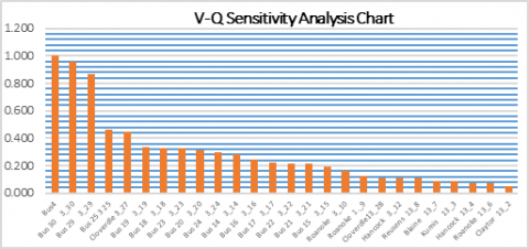
Sensitivity analysis method: This analysis identifies the weakest regions, which represent the highest sensitivity (#1), to (#30), which represent the most stable regions according to the model used. These regions are then arranged from 1 to 30 in order, from weakest to strongest, as shown in Figure 13, in the IEEE 30 Bus standards. This is detailed in the Table 2 [22].
(a) For all buses
(b) For seven buses only
Figure 13. Flow charts of sensitivity analysis
Table 2. V-Q sensitivity analysis report
|
Bus ID |
kV |
Rank # |
V-Q Sensitivity |
|
Bus4 |
33 |
1 |
1.000 |
|
Bus 30 3_30 |
33 |
2 |
0.959 |
|
Bus 29 3_29 |
33 |
3 |
0.867 |
|
Bus 25 3 25 |
33 |
4 |
0.463 |
|
Cloverdle 3_27 |
33 |
5 |
0.446 |
|
Bus 19 3_19 |
33 |
6 |
0.334 |
|
Bus 18 3_18 |
33 |
7 |
0.327 |
|
Bus 23 3_23 |
33 |
8 |
0.323 |
|
Bus 20 3_20 |
33 |
9 |
0.313 |
|
Bus 24 3_24 |
33 |
10 |
0.293 |
|
Bus 14 3_14 |
33 |
11 |
0.281 |
|
Bus 16 3_16 |
33 |
12 |
0.242 |
|
Bus 17 3_17 |
33 |
13 |
0.219 |
|
Bus 22 3_22 |
33 |
14 |
0.214 |
|
Bus 21 3 21 |
33 |
15 |
0.212 |
|
Bus 15 3_15 |
33 |
16 |
0.192 |
|
Roanoke 3_10 |
33 |
17 |
0.159 |
|
Roanoke 1.9 |
33 |
18 |
0.121 |
|
Cloverdle13_28 |
132 |
19 |
0.112 |
|
Hancock 3_12 |
33 |
20 |
0.107 |
|
Reusens 13_8 |
132 |
21 |
0.106 |
|
Blaine 13_7 |
132 |
22 |
0.090 |
|
Kumis 13_3 |
132 |
23 |
0.088 |
|
Hancock 13_4 |
132 |
24 |
0.070 |
|
Roanoke 13_6 |
132 |
25 |
0.068 |
|
Roanoke 1_9 |
33 |
26 |
0.053 |
|
Roanoke 3_10 |
33 |
27 |
0.049 |
|
Claytor 13_2 |
132 |
28 |
0.045 |
|
Hancock 1_13 |
11 |
29 |
0.012 |
|
Bus68 |
11 |
30 |
0.0036 |
PV-QV analysis method: The traditional method through which the load flow analysis is carried out, with the possibility of adding or removing loads, where the active power, reactive power, power factor, and other Factors are calculated. As shown in Figure 14.
Figure 14. P-V and Q-V voltage stability analysis
Table 3 presents the P-V analysis with summary results, as the detailed results of this analysis are extensive. A summary of the analysis is provided in the following table.
Table 3. P-V voltage stability analysis summary report
|
Load Variation Pattern |
Constant PF |
Load Variation Location |
Study Bus Only |
|||
|
Bus |
kV |
Load Variation |
Operating Load |
Maximum Load |
||
|
ID |
%V |
P (MW) |
%V |
P (MW) |
||
|
Blaine 13_7 |
132 |
Yes |
100.2 |
22.800 |
62.1 |
157.941 |
|
Bus 14 3_14 |
33 |
Yes |
104.2 |
6.200 |
63.3 |
79.888 |
|
Bus 15 3_15 |
33 |
Yes |
103.8 |
8.200 |
66.3 |
95.655 |
|
Bus 16 3_16 |
33 |
Yes |
104.4 |
3.500 |
62.6 |
78.277 |
|
Bus 17 3_17 |
33 |
Yes |
104.0 |
9.000 |
63.4 |
81.389 |
|
Bus 18 3_18 |
33 |
Yes |
102.8 |
3.200 |
64.1 |
72.589 |
|
Bus 19 3_19 |
33 |
Yes |
102.6 |
9.500 |
64.0 |
74.508 |
|
Bus 20 3_20 |
33 |
Yes |
103.0 |
2.200 |
63.5 |
73.539 |
|
Bus 21 3_21 |
33 |
Yes |
103.3 |
17.500 |
63.1 |
88.588 |
|
Bus 22 3_22 |
33 |
Yes |
103.3 |
0.000 |
65.1 |
86.350 |
|
Bus 23 3_23 |
33 |
Yes |
102.7 |
3.200 |
60.9 |
63.894 |
|
Bus 24 3_24 |
33 |
Yes |
102.1 |
8.700 |
63.5 |
83.610 |
|
Bus 25 3 25 |
33 |
Yes |
101.7 |
0.000 |
60.7 |
58.163 |
|
Bus 29 3_29 |
33 |
Yes |
100.4 |
2.400 |
59.9 |
36.526 |
|
Bus 30 3_30 |
33 |
Yes |
99.2 |
10.600 |
61.6 |
43.812 |
|
Bus4 |
33 |
Yes |
100.0 |
3.500 |
55.2 |
26.836 |
|
Bus68 |
11 |
Yes |
108.2 |
0.000 |
67.5 |
86.066 |
|
Claytor 13_2 |
132 |
Yes |
104.3 |
21.700 |
67.3 |
429.534 |
|
Cloverdle 3_27 |
33 |
Yes |
102.3 |
0.000 |
65.3 |
65.409 |
|
Cloverdle13_28 |
132 |
Yes |
100.7 |
0.000 |
65.0 |
160.358 |
|
Fieldale 13_5 |
132 |
Yes |
101.0 |
94.200 |
65.7 |
236.387 |
|
Hancock 1_13 |
11 |
Yes |
107.1 |
0.000 |
68.9 |
87.418 |
|
Hancock 3_12 |
33 |
Yes |
105.7 |
11.200 |
65.9 |
96.923 |
|
Hancock 13_4 |
132 |
Yes |
101.2 |
7.600 |
67.5 |
271.246 |
|
Kumis 13_3 |
132 |
Yes |
102.1 |
2.400 |
63.8 |
245.204 |
|
Reusens 13_8 |
132 |
Yes |
100.9 |
30.000 |
62.1 |
140.958 |
|
Roanoke 3_10 |
33 |
Yes |
104.5 |
5.802 |
133.3 |
101.117 |
|
Roanoke 1_9 |
33 |
Yes |
105.1 |
0.000 |
68.1 |
116.665 |
|
Roanoke 13_6 |
132 |
Yes |
101.0 |
0.000 |
67.8 |
196.093 |
6.2 Voltage stability analysis (with EV charging station)
After completing the modeling of the vehicle and charger loads in the IEEE 30-bus system, we will proceed to integrate them into this system. We will work on two paths:
First: Connect the chargers to 33 kV (the weakest buses of the system according to the Sensitivity analysis, as shown highlighted in green in Table 2) using auxiliary transformers, and observe their impact on the system.
Second: Add the chargers to 11 kV (the strongest buses of the system, according to the Sensitivity analysis, as shown highlighted in green in Table 2) using conventional transformers, and observe their impact on the system.
6.2.1 Voltage stability analysis in weak regions
After modeling the electric vehicle and charging stations using ETAP, five charging stations were added to the system (according to the IEEE 30 Bus standard). Vehicles were then added in different numbers and with different load ratios to these stations. Let's assume that we randomly selected the first charger for five electric vehicles, the second for two cars, the third for one truck, the fourth for four vehicles, and the last for three vehicles, with different charging methods and levels, as shown in Figure 15. The selection of these buses to add chargers came after an in-depth analysis to determine the extent of the impact of increased load on the most sensitive Regions. Table 4 and Figure 16 illustrate the results of this impact.
Figure 15. EVs and EVCSs modeling in ETAP
Table 4. V-Q sensitivity analysis report
|
V-Q Sensitivity Analysis Report |
|||
|
Bus ID |
kV |
Rank # |
V-Q Sensitivity |
|
Bus23 |
0.38 |
1 |
1.000 |
|
Bus24 |
0.38 |
2 |
0.983 |
|
Bus18 |
0.38 |
3 |
0.974 |
|
Bus91 |
0.38 |
4 |
0.925 |
|
Bus90 |
0.38 |
5 |
0.914 |
|
Bus4 |
33 |
150 |
0.012 |
|
Bus 30 3_30 |
33 |
151 |
0.011 |
|
Bus 29 3_29 |
33 |
152 |
0.010 |
|
Bus 25 3 25 |
33 |
153 |
0.005 |
|
Cloverdle 3_27 |
33 |
154 |
0.005 |
|
Bus 19 3_19 |
33 |
155 |
0.004 |
|
Bus 18 3_18 |
33 |
156 |
0.004 |
|
Bus 23 3_23 |
33 |
157 |
0.004 |
|
Bus 20 3_20 |
33 |
158 |
0.004 |
|
Bus 24 3_24 |
33 |
159 |
0.003 |
|
Bus 14 3_14 |
33 |
160 |
0.003 |
|
Bus 16 3_16 |
33 |
161 |
0.003 |
|
Bus 17 3_17 |
33 |
162 |
0.003 |
|
Bus 22 3_22 |
33 |
163 |
0.002 |
|
Bus 21 3_21 |
33 |
164 |
0.002 |
|
Bus 15 3_15 |
33 |
165 |
0.002 |
|
Roanoke 1_9 |
33 |
167 |
0.001 |
|
Cloverdle13_28 |
132 |
168 |
0.001 |
|
Hancock 3_12 |
33 |
169 |
0.001 |
|
Reusens 13_8 |
132 |
170 |
0.001 |
|
Blaine 13_7 |
132 |
171 |
0.001 |
|
Kumis 13_3 |
132 |
172 |
0.001 |
|
Hancock 13_4 |
132 |
173 |
0.001 |
|
Roanoke 13_6 |
132 |
174 |
0.001 |
|
Claytor 13_2 |
132 |
175 |
0.001 |
Figure 16. The weakest buses in the system after the addition of EVCS
Sensitivity analysis was performed, and it was noted that the additional five buses (created by connecting the chargers to the system) were identified as the weakest buses, as indicated in gray below in Table 4 (this analysis was performed with the charger loaded at 100%).
And Figure 16 will display the chart for the analysis in Table 4.
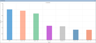
After identifying the new weak Regions that have been added to the system, which are the five charger areas in grey color as shown in Table 4, perform a P-V voltage stability analysis by changing the load ratios for the chargers from 0% to 100%. To clearly observe the impact of adding chargers, as shown in Table 5. The results in this table were obtained by reducing a large table with huge values by varying the load percentage from 0%, which represents the system without any additional effects (as if the chargers were canceled), to 100% in 20% steps. Convert it to a smaller table with values that can be displayed throughout the paper (0%, 40%, 80%, and 100%). To match the paper format.
Table 5. An increase in load chargers with the voltage stability index (Ranks from #1 to #10)
|
Loading |
0% |
40% |
80% |
100% |
|
#1 |
99.04 |
95.65 |
91.93 |
89.92 |
|
#2 |
99.83 |
96.48 |
92.82 |
90.84 |
|
#3 |
100.2 |
96.85 |
93.19 |
91.22 |
|
#4 |
101.6 |
98.41 |
94.92 |
93.04 |
|
#5 |
102.2 |
98.97 |
95.48 |
93.61 |
|
#6 |
99.83 |
99.6 |
99.34 |
99.2 |
|
#7 |
99.04 |
98.79 |
98.52 |
98.36 |
|
#8 |
100.2 |
99.95 |
99.69 |
99.54 |
|
#9 |
101.6 |
101.4 |
101.2 |
101.1 |
|
#10 |
102.2 |
102 |
101.8 |
101.7 |
And below the P-V analysis Table 6, at 100% charging loads, with exact values shown for each bus.
Table 6. P-V analysis summary after adding EV charging station
|
P-V Analysis Summary |
||||||
|
Load Variation Pattern |
Constant PF |
Load Variation Location |
Study Bus Only |
|||
|
Bus |
kV |
Load Variation |
Operating Load |
Maximum Load |
||
|
ID |
%V |
P (MW) |
%V |
P (MW) |
||
|
Blaine 13_7 |
132 |
Yes |
100.1 |
22.800 |
62.3 |
155.228 |
|
Bus 14 3_14 |
33 |
Yes |
104.1 |
6.200 |
63.4 |
78.647 |
|
Bus 15 3_15 |
33 |
Yes |
103.6 |
8.200 |
66.2 |
93.825 |
|
Bus 16 3_16 |
33 |
Yes |
104.3 |
3.500 |
62.5 |
76.854 |
|
Bus 17 3_17 |
33 |
Yes |
103.8 |
9.000 |
62.9 |
79.824 |
|
Bus 18 3_18 |
33 |
Yes |
102.6 |
3.200 |
63.4 |
71.319 |
|
Bus 19 3_19 |
33 |
Yes |
102.4 |
9.500 |
62.6 |
73.343 |
|
Bus 20 3_20 |
33 |
Yes |
102.8 |
2.200 |
62.8 |
72.166 |
|
Bus 21 3_21 |
33 |
Yes |
103.0 |
17.500 |
62.9 |
86.869 |
|
Bus 22 3_22 |
33 |
Yes |
103.1 |
0.000 |
65.2 |
84.143 |
|
Bus 23 3_23 |
33 |
Yes |
102.5 |
3.200 |
59.9 |
62.629 |
|
Bus 24 3_24 |
33 |
Yes |
101.8 |
8.700 |
63.5 |
81.571 |
|
Bus 25 3 25 |
33 |
Yes |
101.1 |
0.000 |
61.3 |
55.615 |
|
Bus 29 3_29 |
33 |
Yes |
99.5 |
2.400 |
59.7 |
35.008 |
|
Bus 30 3_30 |
33 |
Yes |
98.4 |
10.600 |
62.4 |
42.337 |
|
Bus18-1 |
0.38 |
Yes |
91.2 |
0.253 |
53.9 |
0.752 |
|
Bus23-1 |
0.38 |
Yes |
89.9 |
0.253 |
52.6 |
0.734 |
|
Bus24-1 |
0.38 |
Yes |
90.8 |
0.253 |
50.6 |
0.745 |
|
Bus4 |
33 |
Yes |
99.2 |
3.500 |
56.9 |
25.805 |
|
Bus68 |
11 |
Yes |
108.2 |
0.000 |
67.4 |
84.584 |
|
Bus90-1 |
0.38 |
Yes |
93.0 |
0.253 |
54.2 |
0.775 |
|
Bus91-1 |
0.38 |
Yes |
93.6 |
0.253 |
52.6 |
0.795 |
|
Claytor 13_2 |
132 |
Yes |
104.2 |
21.700 |
69.5 |
420.196 |
|
Cloverdle 3_27 |
33 |
Yes |
101.7 |
0.000 |
65.6 |
62.378 |
|
Cloverdle13_28 |
132 |
Yes |
100.4 |
0.000 |
65.6 |
155.142 |
|
Fieldale 13_5 |
132 |
Yes |
101.0 |
94.200 |
65.5 |
234.308 |
|
Glen Lyn 13_1 |
132 |
Yes |
106.0 |
0.000 |
106.0 |
17001.757 |
|
Hancock 1_13 |
11 |
Yes |
107.1 |
0.000 |
68.5 |
85.871 |
|
Hancock 3_12 |
33 |
Yes |
105.6 |
11.200 |
66.0 |
95.109 |
|
Hancock 13_4 |
132 |
Yes |
101.0 |
7.600 |
68.7 |
264.936 |
|
Kumis 13_3 |
132 |
Yes |
101.9 |
2.400 |
64.0 |
240.510 |
|
Reusens 13_8 |
132 |
Yes |
100.6 |
30.000 |
62.7 |
137.148 |
|
Roanoke 1_9 |
33 |
Yes |
104.9 |
0.000 |
68.7 |
113.756 |
|
Roanoke 13_6 |
132 |
Yes |
100.8 |
0.000 |
68.1 |
190.134 |
6.2.2 Voltage stability analysis for 11 kV buses
It is worth noting that there are two 11 kV buses with the highest Ranks (Hancock 1-13 and Bus68), as shown in the sensitivity analysis Table 2. These two buses have the highest stability index, and adding heavy loads to them (chargers and their components), increasing and doubling them as shown in Figure 17. will not lead to a clear effect on them, as shown in Table 7. As for the working mechanism, five chargers with the maximum possible capacity (Loading 100%) were placed on each bus (Hancock 1-13 and Bus 68) and connected to the system through a 5 MVA, 2-winding transformer, as shown in Figure 17.
Figure 17. The chargers and EVs are connected to 11 kV buses
We note from the voltage stability analysis that the effect of the chargers is very slight, and the buses remained highly stable even after doubling the loads two and three times. Table 7 illustrates the voltage stability analysis in the scenario with five chargers on the two buses depicted in Figure 17.
Table 7. P-V analysis summary when charger connected to 11 kV
|
P-V Analysis Summary |
||||||
|
Load Variation Pattern |
Constant PF |
Load Variation Location |
Study Bus Only |
|||
|
Bus |
kV |
Load Variation |
Operating Load |
Maximum Load |
||
|
ID |
%V |
P (MW) |
%V |
P (MW) |
||
|
Blaine 13_7 |
132 |
Yes |
100.1 |
22.800 |
62.0 |
154.998 |
|
Bus 14 3_14 |
33 |
Yes |
104.1 |
6.200 |
63.3 |
78.027 |
|
Bus 15 3_15 |
33 |
Yes |
103.6 |
8.200 |
65.7 |
93.146 |
|
Bus 16 3_16 |
33 |
Yes |
104.3 |
3.500 |
62.8 |
76.266 |
|
Bus 17 3_17 |
33 |
Yes |
103.8 |
9.000 |
62.6 |
79.367 |
|
Bus 18 3_18 |
33 |
Yes |
102.7 |
3.200 |
63.0 |
70.859 |
|
Bus 19 3_19 |
33 |
Yes |
102.4 |
9.500 |
62.9 |
72.892 |
|
Bus 20 3_20 |
33 |
Yes |
102.8 |
2.200 |
63.8 |
71.660 |
|
Bus 21 3_21 |
33 |
Yes |
103.1 |
17.500 |
62.8 |
86.540 |
|
Bus 22 3_22 |
33 |
Yes |
103.2 |
0.000 |
65.3 |
83.650 |
|
Bus 23 3_23 |
33 |
Yes |
102.6 |
3.200 |
60.4 |
62.374 |
|
Bus 24 3_24 |
33 |
Yes |
102.0 |
8.700 |
63.2 |
81.638 |
|
Bus 25 3 25 |
33 |
Yes |
101.6 |
0.000 |
60.5 |
56.752 |
|
Bus 29 3_29 |
33 |
Yes |
100.1 |
2.400 |
58.9 |
35.885 |
|
Bus 30 3_30 |
33 |
Yes |
99.0 |
10.600 |
61.2 |
43.149 |
|
Bus4 |
33 |
Yes |
99.8 |
3.500 |
61.4 |
26.018 |
|
Bus68 |
11 |
Yes |
108.2 |
0.000 |
68.5 |
83.052 |
|
Bus91-3 |
0.38 |
Yes |
106.9 |
1.263 |
63.1 |
17.178 |
|
Bus91-5 |
0.38 |
Yes |
105.8 |
1.263 |
60.6 |
17.391 |
|
Claytor 13_2 |
132 |
Yes |
104.2 |
21.700 |
67.8 |
421.927 |
|
Cloverdle 3_27 |
33 |
Yes |
102.1 |
0.000 |
63.3 |
63.926 |
|
Cloverdle13_28 |
132 |
Yes |
100.5 |
0.000 |
64.7 |
155.727 |
|
Fieldale 13_5 |
132 |
Yes |
101.0 |
94.200 |
65.6 |
233.946 |
|
Glen Lyn 13_1 |
132 |
Yes |
106.0 |
0.000 |
106.0 |
16992.781 |
|
Hancock 1_13 |
11 |
Yes |
107.1 |
0.000 |
68.4 |
84.421 |
|
Hancock 3_12 |
33 |
Yes |
105.6 |
11.200 |
65.4 |
94.241 |
|
Hancock 13_4 |
132 |
Yes |
101.0 |
7.600 |
68.3 |
264.620 |
|
Kumis 13_3 |
132 |
Yes |
101.9 |
2.400 |
64.2 |
240.176 |
|
Reusens 13_8 |
132 |
Yes |
100.6 |
30.000 |
61.0 |
137.754 |
|
Roanoke 1_9 |
33 |
Yes |
105.0 |
0.000 |
67.8 |
112.769 |
|
Roanoke 13_6 |
132 |
Yes |
100.8 |
0.000 |
67.4 |
190.203 |
This study provides a quantitative assessment of how electric vehicle charging stations impact voltage stability, utilizing the IEEE 30-bus system as a realistic model. Our results lead to an indisputable conclusion: charger placement is as important as charger size.
Our preliminary analysis provides clear information for ranking the system's buses from weakest to strongest. The V-Q sensitivity analysis clearly identified bus 4 (33 kV) as the most vulnerable node with a sensitivity value of 1.000, while bus 68 (11 kV) was the most stable with a value of just 0.0036.
The results provided a crucial assessment when we connected five high-power (240 kW) DC fast-charging stations to the weakest 33 kV buses. The impact was severe and immediate, while the voltage stability of these new charging buses declined sharply, becoming the most vulnerable point in the entire system. For example, in some areas of the grid, when these chargers were operating at full capacity (100%), the voltage on these buses dropped to extremely low levels. Bus 23-1 reached only 89.9% of its rated voltage, and its maximum load capacity dropped to just 0.734 MW. This represents a severe performance degradation, pushing the system toward the limits of instability. Adding the same large charging load to the two most powerful 11 kV buses (Hankook 1_13 and Bus 68) had no significant effect. Even under full load, Bus 68's voltage remained at a healthy 108.2%, and its load-carrying capacity remained virtually unchanged, reaching a maximum load capacity of 83.052 MW. This demonstrates that the stronger parts of the grid can easily accommodate this new demand.
However, the vulnerability of weaker buses should not be viewed as merely an obstacle; rather, it identifies critical areas that require attention. These sensitive nodes represent prime candidates for targeted infrastructure upgrades, such as installing capacitor banks to support reactive power or reinforcing the grid, to increase their capacity. In this way, the challenge of EV integration can be transformed into an opportunity to strengthen the entire power system proactively.
While the unplanned addition of EV chargers poses a threat to grid stability, a smart, data-driven approach that combines the strategic deployment of robust buses with targeted reinforcement of weak buses not only mitigates risks but also enhances overall system resilience.
[1] Eltoumi, F. (2020). Charging station for electric vehicle using hybrid sources. https://theses.hal.science/tel-03145375v1.
[2] Çelik, S., Ok, Ş. (2024). Electric vehicle charging stations: Model, algorithm, simulation, location, and capacity planning. Heliyon, 10(7): e29153. https://doi.org/10.1016/j.heliyon.2024.e29153
[3] Mastoi, M.S., Zhuang, S.X., Munir, H.M., Haris, M., Hassan, M., Usman, M., Bukhari, S.S.H., Ro, J.S. (2022). An in-depth analysis of electric vehicle charging station infrastructure, policy implications, and future trends. Energy Reports, 8: 11504-11529. https://doi.org/10.1016/j.egyr.2022.09.011
[4] Acharige, S.S.G., Haque, M.E., Arif, M.T., Hosseinzadeh, N., Hasan, K.N., Oo, A.M.T. (2023). Review of electric vehicle charging technologies, standards, architectures, and converter configurations. IEEE Access, 11: 41218-41255. https://doi.org/10.1109/ACCESS.2023.3267164
[5] Saraswathi, V.N., Ramachandran, V.P. (2024). A comprehensive review on charger technologies, types, and charging stations models for electric vehicles. Heliyon, 10(20): e38945. https://doi.org/10.1016/j.heliyon.2024.e38945
[6] Kumar, M., Panda, K.P., Naayagi, R.T., Thakur, R., Panda, G. (2023). Comprehensive review of electric vehicle technology and its impacts: Detailed investigation of charging infrastructure, power management, and control techniques. Applied Sciences, 13(15): 8919. https://doi.org/10.3390/app13158919
[7] Huaman-Rivera, A., Calloquispe-Huallpa, R., Luna Hernandez, A.C., Irizarry-Rivera, A. (2024). An overview of electric vehicle load modeling strategies for grid integration studies. Electronics, 13(12): 2259. https://doi.org/10.3390/electronics13122259
[8] Nour, M., Chaves-Ávila, J.P., Magdy, G., Sánchez-Miralles, Á. (2020). Review of positive and negative impacts of electric vehicles charging on electric power systems. Energies, 13(18): 4675. https://doi.org/10.3390/en13184675
[9] Panatarani, C., Murtaddo, D., Maulana, D.W., Irawan, S., Joni, I.M. (2016). Design and development of electric vehicle charging station equipped with RFID. AIP Conference Proceedings, 1712(1): 030007. https://doi.org/10.1063/1.4941872
[10] Tavakoli, A., Saha, S., Arif, M.T., Haque, M.E., Mendis, N., Oo, A.M.T. (2020). Impacts of grid integration of solar PV and electric vehicle on grid stability, power quality and energy economics: A review. IET Energy Systems Integration, 2(3): 215-225. https://doi.org/10.1049/iet-esi.2019.0047
[11] Shivakumar, P., Barik, S.K. (2022). Implementation of SVM based multi-level inverter for grid connected PV system. Journal Européen des Systèmes Automatisés, 55(3): 413-418. https://doi.org/10.18280/jesa.550314
[12] Srivastava, A., Manas, M., Dubey, R.K. (2023). Electric vehicle integration’s impacts on power quality in distribution network and associated mitigation measures: A review. Journal of Engineering and Applied Science, 70: 32. https://doi.org/10.1186/s44147-023-00193-w
[13] Dharmakeerthi, C.H., Mithulananthan, N., Saha, T.K. (2014). Impact of electric vehicle fast charging on power system voltage stability. International Journal of Electrical Power & Energy Systems, 57: 241-249. https://doi.org/10.1016/j.ijepes.2013.12.005
[14] Dhayanandh, S., Ramakrishnan, K.C., Reddy, V.S.N., Bhaskar, S.U. (2021). Impact of the power grid on charging stations of various power rating and sizes. Revista Gestão Inovação e Tecnologias, 11(3): 1589-1605. https://revistageintec.net/old/wp-content/uploads/2022/02/2033.pdf.
[15] K, N.K., S, J.N., Jadoun, V.K. (2023). Optimization of distribution network operating parameters in grid tied microgrid with electric vehicle charging station placement and sizing in the presence of uncertainties. International Journal of Green Energy, 22(8): 1552-1569. https://doi.org/10.1080/15435075.2023.2281334
[16] Gómez-Ramírez, G.A., Solis-Ortega, R., Ross-Lépiz, L.A. (2023). Impact of electric vehicles on power transmission grids. Heliyon, 9(11): e22253. https://doi.org/10.1016/j.heliyon.2023.e22253
[17] Apata, O., Bokoro, P.N., Sharma, G. (2023). The risks and challenges of electric vehicle integration into smart cities. Energies, 16(14): 5274. https://doi.org/10.3390/en16145274
[18] Tounsi Fokui, W.S., Saulo, M., Ngoo, L. (2022). Controlled electric vehicle charging for reverse power flow correction in the distribution network with high photovoltaic penetration: Case of an expanded IEEE 13 node test network. Heliyon, 8(3): e09058. https://doi.org/10.1016/j.heliyon.2022.e09058
[19] Intel Corporation. (2022). Electric Vehicle (EV) Charging: The Missing Link for Smart, Sustainable Cities. https://builders.intel.com/docs/networkbuilders/electric-vehicle-ev-charging-the-missing-link-for-smart-sustainable-cities-1723023278.pdf.
[20] Kumar, S., Usman, A., Rajpurohit, B.S. (2021). Battery charging topology, infrastructure, and standards for electric vehicle applications: A comprehensive review. IET Energy Systems Integration, 3(4): 381-396. https://doi.org/10.1049/esi2.12038
[21] Wilkenfeld, G. (2021). Evaluating international standards for electric vehicle chargers for SA Department for Energy and Mining. George Wilkenfeld and Associates. https://www.energymining.sa.gov.au/__data/assets/pdf_file/0003/813522/Evaluating-international-standards-for-electric-vehicle-chargers-George-Wilkenfeld-and-Associates-with-Auseng-Pty-Ltd-December-2021.pdf.
[22] Begovic, M., Bright, J., Domin, T., Ibrahim, M., et al. (1996). Voltage collapse mitigation report to IEEE Power System Relaying Committee. IEEE PSRC. https://www.pes-psrc.org/kb/report/012.pdf.