Antonio Rosato![]() | Achille Perrotta*
| Achille Perrotta*![]() | Tania Bracchi
| Tania Bracchi![]() | Luigi Maffei
| Luigi Maffei![]()
© 2025 The authors. This article is published by IIETA and is licensed under the CC BY 4.0 license (http://creativecommons.org/licenses/by/4.0/).
OPEN ACCESS
The performance of three commercial small-scale wind turbines (SWTs) serving a typical house have been analyzed via the software TRNSYS upon varying the climatic conditions of 5 Italian and 3 Norwegian cities. A Savonius vertical axis SWT (power output of 2100 W at 12 m/s and rotor swept area equal to 1.60 m2) has been compared with two horizontal axis SWTs, the first one characterized by the same power output at 12 m/s (but 3.8 times larger rotor swept area) and the second one with almost equal rotor swept area (but 6.8 times lower power output at 12 m/s). The selected SWTs have been compared with a baseline scenario where the same building is served by the central electric grid only from energy, environmental and economic points of view. The simulations highlighted that the vertical axis SWT produces 1.05÷11.54 times larger annual electric energy than the horizontal axis SWTs. The data also underlined that, with respect to the baseline scenario, the selected SWTs reduce annual electric energy imported from grid (up to 37.5%), the equivalent global CO2 emissions (up to 37.8%) and the operating costs (up to 112%), with a minimum simple payback period of 2.8 years.
small-scale vertical wind turbines, small-scale horizontal wind turbines, TRNSYS, renewable energy sources, energy efficiency in buildings
Fossil fuel usage and greenhouse gas emissions are increasing, and the International Energy Agency has highlighted that residential applications account for the bulk of global energy consumption [1]. EU members must guarantee that average energy demand of residential sector decreases by at least 16% by 2030 (based on the new Energy Performance of Buildings Directive). With reference to this prospective, it is well known that promoting the utilization of renewable sources is one of the most promising approaches to reduce primary energy demand and mitigate climate change [1, 2]. Many nations enhanced the adoption of technologies based on renewable sources in order to produce clean energy to meet their increasing demands. Wind energy is among the most widely used renewable sources [2]. One of the renewable energy source-based solutions that is rapidly gaining a lot of attention from the scientific community in recent decades is the use of wind turbines (WTs) to convert wind energy into power [2-4]. Rated power output of WTs is generally used for their categorization as follows [5]: (i) small-scale WTs, (ii) medium-scale, (iii) large-scale WTs. Small-scale wind turbines (SWTs) are those having an electric output up to 50 kW together with a rotor swept area (i.e., the area within which a wind turbine's blades rotate) lower than 200 m2, according to the study [6]. SWTs are situated near or on the "customer" side of the area where the power they generate is utilized. SWTs are often used in small-scale commercial, industrial, and agricultural contexts; however, because they can be installed even in certain urban areas, they are also a good choice for homeowners [3, 5]. They can be utilized to meet the on-site load or directly connected to the central grid. Additionally, they may be used in hybrid energy systems that integrate other technologies (like different energy conversion units, batteries, etc.). Compared to large- and medium-scale WTs, SWTs can offer a number of potential advantages, such as reduced maintenance costs, improved reliability, a greater range of wind speeds at which they can operate, a smaller installation space requirement, less dependence on grid-connected power and long transmission lines, lower capital costs, etc; SWTs might therefore be used and incorporated into urban residential settings. Even with these possible advantages, building-integrated SWTs can be difficult to design and efficiently run. First and foremost, it should be considered that the potential of SWTs is dependent on various factors, such as wind speed and installation site. From this perspective, the presence of various physical obstacles, such as buildings and trees, can make it challenging to create a consistent energy source in urban settings [3, 5, 7]. Additionally, a real SWT is exposed to wind that abruptly changes speed and/or direction; manufacturers’ power curves typically do not take into account such transient operation and related efficiency losses. The performance of SWT may be significantly impacted by these factors [3, 5, 7, 8]. SWTs may be broadly categorized into two main categories [9]: (i) vertical axis small-scale wind turbines (VASWTs); and (ii) horizontal axis small-scale turbines (HASWTs). VASWTs are distinguished by an axis of rotation that is perpendicular to the wind flow, whereas HASWTs have an axis of rotation that is parallel to the wind flow. HASWTs rely on the direction of the wind to function, but VASWTs are omnidirectional in their operation taking into account that they can use wind from any direction [9, 10]. Based on the rotor type, VASWTs may be categorized into two sub-categories [11]: the drag-based Savonius models and the lift-based Darrieus models. A hybrid Savonius-Darrieus design can be also recognized. It can be highlighted that there are very few scientific studies in the literature that have compared vertical and horizontal SWTs with the same rotor swept area or rated electrical power. For example, Fadil and Ashari [12] compared a VASWT with a HASWT (not commercial models) characterized by the same rotor swept area (3.14 m2) and blades (3); they found a maximum power output of 1363.6 W and 505.69 W, respectively, for the HASWT and the VASWT.
In this work, the performance of the following 3 commercial SWTs have been analyzed:
The above-mentioned VASWT has been selected taking into account that its performance has been already analyzed by the authors in previously published scientific papers [16-18], where its energy, environmental and economic suitability have been demonstrated. The other two SWTs have been considered in this study with the aim of compare the performance of the selected VASWT with a HASWT characterized by the same power output at 12 m/s (but 3.8 times larger rotor swept area) as well as with a HASWT characterized by a very similar (differing by about 10%) rotor swept area (but 6.8 times lower power output at 12 m/s). The performance of the above-mentioned SWTs have been assessed via the dynamic TRaNsient SYStems simulation tool (TRNSYS) [19] (version 18) while serving the same typical single-family house (assumed as reference) upon varying the locations; in particular, 5 different cities in Italy (Alghero, Milan, Naples, Palermo, Rome) and 3 Norwegian cities (Bergen, Karasjok, Tromsø) have been considered. The annual power demand profile associated to the operation of lighting systems and domestic appliances of the house has been defined via a stochastic tool [20]; in addition, wind velocity profiles corresponding to urban settings have been considered by means of a specific TRNSYS mathematical model. The energy, environmental and economic performance of the building-integrated SWTs have been contrasted with that one of a baseline scenario (where the electric demand of the same house is totally covered by the central grid only) with the aim of assessing the potential benefits in terms of imported electric energy, equivalent global CO2 emissions as well as operating costs. The simple payback period has been also evaluated. The main goals of the paper can be summarized as reported below:
Section 2 details the electric load profile of the building, the selected SWTs’ models, as well as the simulation model and the corresponding climatic data used for running the simulations; Section 3 reports the simulations results, while Section 4 compares the energy, environmental and economic performance of the selected SWTs with respect to a baseline scenario without SWTs.
This section of the paper describes the electric demand of the residential building assumed as reference (Section 2.1), the characteristics of the selected horizontal and vertical SWTs (Section 2.2), as well as the mathematical models adopted for simulating the SWTs as well as the climatic conditions (Section 2.3).
2.1 Building electric demand
It is commonly recognized that a wide range of factors influence how much electricity homeowners use. In order to predict the corresponding daily electric energy demand profiles linked to the operation of lighting systems and household appliances, an original tool created by Loughborough University based on a stochastic method [20] has been applied in this work. The maximum number of occupants, the day of the week or weekend, the month of the year, and the quantity and kind of household appliances can all be used to generate these daily profiles. The electric demand for cooking appliances, water heating, and air conditioning systems is not taken into consideration by this tool. The associated daily electric profile is then computed based on the actual number of people and the random activations of the lighting and household appliances. Profiles that may be regarded as representative of common homes can be obtained using this method [21]. In this study, in particular, a maximum of 4 people is assumed and the most commonly used domestic appliances have been considered. The annual electric demand of the house considered assumed as reference in this study has been defined by combining 365 different daily electric demand profiles obtained via the above-mentioned tool [20] with a time-step equal to 1 minute. Figure 1 reports both the annual electric demand profile as a function of the time (black curve) as well as the corresponding electric load-duration diagram with the values sorted in descending order (red curve). The annual electric energy required by the building assumed as reference is 2408.96 kWh.
Figure 1. Annual electric demand profile and load-duration profile of the residential building
2.2 Wind turbines
Three commercial SWTs (a Savonius SWT with vertical axis [13], and two SWTs with horizontal axis [14, 15]) have been investigated in this work. Table 1 reports the axis type (horizontal or vertical), manufacturer, model, power output at 12 m/s, rotor swept area, rotor diameter, blades height (for the VASWT only), number of blades, cut-in wind speed (i.e., the minimum wind speed at which the SWTs begin providing an usable electric power), cut-out wind speed (i.e., the highest wind speed at which the SWTs are intended to produce useable electric energy), and capital cost of the selected SWTs. The rotor swept area of the HASWTs is given as pR2 (where R is the rotor radius), while for the Savonius VASWT it is calculated as DH (where D is the rotor diameter (equal to 0.80 m) and H is the blades height (equal to 2.0 m)) [12]. This table indicates that the rotor swept area of the HASWT FK-2000 is 3.8 and 4.3 times larger than that one of the VASWT FS-2000 and the HASWT ATO-WT-NE-300S5, respectively. Figure 2 reports the power curves of the selected SWTs according to the data provided by the manufacturers; these curves show the operating ranges of both wind speed (from the cut-in up to the cut-out) and power output of the SWTs. This figure shows that:
Table 1. Selected SWTs
|
|
VASWT [13] |
HASWT [14] |
HASWT [15] |
|
Axis type |
Vertical |
Horizontal |
Horizontal |
|
Manufacturer |
FLTXNY |
FLTXNY |
ATO |
|
Model |
FS-2000 |
FK-2000 |
ATO-WT-NE-300S5 |
|
Power output at 12 m/s (kW) |
2.100 |
2.100 |
0.307 |
|
Rotor swept area (m2) |
1.60 |
6.15 |
1.43 |
|
Rotor diameter (m) |
0.80 |
2.80 |
1.35 |
|
Blades height (m) |
2.0 |
- |
- |
|
Blades number |
2 |
3 |
3 |
|
Cut-in wind speed (m/s) |
2 |
3 |
3 |
|
Cut-out wind speed (m/s) |
14 |
12 |
15 |
|
Capital cost (€) |
684.39 |
535.72 |
334.52 |
Figure 2. Power curves of the selected SWTs [13-15]
2.3 Simulation model and climatic data
The TRaNsient SYStems simulation tool (TRNSYS) [19] (version 18) has been adopted in this paper in order to model and simulate the SWTs performance and related climatic conditions. Taking into account that it considers the part-load operation of the energy conversion systems as well as the interactions between electric demand and generation, the platform TRNSYS is usually utilized by the scientific community [22-24]. The TRNSYS library includes a number of mathematical models (called “Types”). In this work, the TRNSYS Type 90 has been considered to model and simulate the performance of the SWTs. This model needs the definition of some parameters (site elevation, data collection height, hub height, turbine power loss) and inputs (wind velocity, ambient temperature, site shear exponent, barometric pressure, control mode, rotor height, rotor diameter, sensor height, turbulence intensity, air density, power rated, speed rated, power curve).
According to the above-mentioned parameters/inputs, the model allows to calculate 3 outputs (power output, power coefficient and time of continuous wind turbine operation). Table 2 summarizes the values assumed in this study for the parameters and inputs of the TRNSYS Type 90 for the SWTs. The SWTs power loss has been considered equal to 0, while a site shear exponent of 0.26 has been adopted with the aim of modelling the scenario corresponding to obstructed airflows (according to the study [25]). The option “P” (i.e., pitched-control) has been selected as control mode for both the HASWTs FK-2000 and ATO-WT-NE-300S5 taking into account that the initial outward pitching manoeuvre serves to reduce the blade’s effective angle of attack, delay the moment when the critical static stall angle is exceeded, and reduce the maximum effective angle of attack [26]. The turbulence intensity is a dimensionless number defined as the standard deviation of wind speeds within a simulation time step divided by the average wind speed over that simulation time step; in this study a value of 10% [27] has been assumed as turbulence intensity, whatever the SWT model is. The weather conditions (site elevation, wind velocity, ambient temperature as well as barometric pressure) required by the TRNSYS Type 90 have been set based on the Typical Meteorological Year version 2 weather database (TMY2) [28] via the TRNSYS Type 15-6. This Type is a weather data processor reading an external weather data file and providing climate conditions representative of the selected cities. In this paper, 5 cities in Italy (Alghero, Milan, Naples, Palermo, Rome) and 3 cities in Norway (Bergen, Karasjok, Tromsø) have been considered as installation sites for the SWTs to take into account the influence of different climatic scenarios on SWTs performance. These cities are characterized by the following coordinates: Alghero (latitude 40° 33' 55.48" North, longitude 8° 19' 15.31" East); Milan (latitude 45° 27' 51.1596'' North, longitude 9° 11' 28.9788'' East); Naples (latitude 40° 51' 11.8584'' North, longitude 14° 18' 20.0628' East); Palermo (latitude 38° 7' 0.0084'' North, longitude 13° 22' 0.0012'' East); Rome (latitude 41° 54' 10.0152'' North, longitude 12° 29' 46.9176'' East); Bergen (latitude 60° 23' 34.4736" North, longitude 5° 19' 27.7788'' East); Karasjok (latitude 69°28' 18" North, longitude 25° 30' 40'' East); Tromsø (latitude 69° 39' 0.9108'' North, longitude 18° 59' 42.4140'' East).
Table 2. Parameters and inputs of the TRNSYS type 90
|
|
FS-2000 |
FK-2000 |
ATO-WT-NE-300S5 |
|
Site elevation (m) |
72 (Naples), 3 (Rome), 211 (Milan), 34 (Palermo), 40 (Alghero), 12 (Bergen), 129 (Karasjok), 102 (Tromsø) |
||
|
Data collection height above ground (m) |
10 |
9 |
9 |
|
Hub height above ground (m) |
9 |
9 |
9 |
|
Turbine power loss (%) |
0 |
0 |
0 |
|
Site shear exponent |
0.26 |
0.26 |
0.26 |
|
Rotor height above ground (m) |
9 |
9 |
9 |
|
Rotor diameter (m) |
0.80 |
2.80 |
1.35 |
|
Sensor height (m) |
10 |
9 |
9 |
|
Turbulence intensity (%) |
10 |
||
|
Air density (kg/m3) |
1.225 |
||
|
Power rated (W) |
2100 |
2100 |
307 |
|
Speed rated (m/s) |
12 |
12 |
12 |
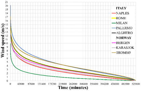
Figure 3 reports the annual wind velocity-duration diagrams upon varying the city (according to study [28]), with the data in descending order. This plot indicates that Palermo is characterized by the largest average annual wind speed (4.24 m/s), while the minimum average annual wind velocity (1.14 m/s) corresponds to the city of Milan.
Figure 3. Annual wind velocity-duration diagrams
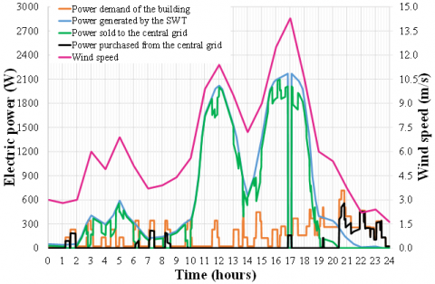
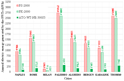
The simulations have been carried out with a simulation time-step of 1 minute over an entire year. The outputs are described in this section. Figure 4 shows an example of daily operation of one of the selected SWTs (VASWT FS-2000) operating in one of the selected cities (Naples) during a specific day (April 15th); in particular, it reports the values of wind speed, power produced by the SWT, building power demand, power produced by the SWT and sold to the grid (in excess with respect to the power demand), power imported from the grid to cover the electric load not covered by the SWT production as a function of the time. Figure 5 indicates the annual electric energy produced by the selected SWTs upon varying both the SWT model and the city. This figure shows that the annual electric generation varies between a minimum of 12.0 kWh (corresponding to the HASWT ATO-WT-NE-300S5 installed in Milan) up to a maximum of 2743.0 kWh (corresponding to the VASWT FS-2000 installed in Palermo). Moreover, it can be underlined that, for a given SWT model, the annual generated electric energy is maximum in the case of the city of Palermo (city characterized by the largest average wind speeds), while it is minimum for the city of Milan (corresponding to the lowest average wind speeds), with values in Palermo between 19.8 and 33.7 times larger than those associated to Milan. The comparison between the VASWT FS-2000 and the HASWT FK-2000 (characterised by the same power output at 12 m/s) shows that, whatever the city is, the VASWT FS-2000 produces larger annual electricity than the HASWT FK-2000 (thanks to the fact that, as indicated in Figure 2, the SWT FS-2000 is characterized by larger power outputs for wind velocities up to 6.5 m/s) by a minimum of 1.05 times (in the case of Tromsø) up to a maximum of 1.80 times (in the case of Milan). In addition, the comparison between the VASWT FS-2000 and the HASWT ATO-WT-NE-300S5 (characterised by almost the same rotor swept area) shows that the VASWT FS-2000 generates greater electric output with respect to the HASWT ATO-WT-NE-300S5 (thanks to the fact that, as reported in Figure 2, the SWT FS-2000 is characterized by a much larger power output, whatever the wind velocity is) by a minimum of 8.47 times (in the case of Palermo) up to a maximum of 11.54 times (in the case of Milan). Finally, it should be underlined that the VASWT FS-2000 is also characterized by a reduced size in comparison to the selected HASWT FK-2000.
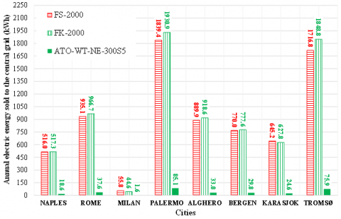
Depending on the simultaneity and levels of electricity production and demand, the output of SWTs could exceed the power demand with the eventual surplus sold to the grid. Figure 6 indicates the annual electric energy sold to the grid upon varying both the SWT model and the city.
Figure 4. Daily operation of the VASWT FS-2000 in Naples on April 15th
Figure 5. Annual generated electric energy
Figure 6. Annual electric energy sold to the central grid
This plot indicates that the values range from a minimum of 1.6 kWh in the case of the HASWT ATO-WT-NE-300S5 operating in Milan up to a maximum of 1930.9 kWh in the case of the HASWT FK-2000 installed in Palermo. For a given city and SWT model, the values reported in Figure 6 represent a significant percentage of the corresponding values of generated electricity (reported in Figure 5); this percentage ranges between 40.3% (in Milan) and 67.1% (in Palermo) for the VASWT FS-2000, between 57.8% (in Milan) and 74.3% (in Palermo) for the HASWT FK-2000, and between 13.4% (in Milan) and 26.3% (in both Tromsø and Palermo) for the HASWT ATO-WT-NE-300S5. These values indicate that coupling the selected SWTs with electric batteries could significantly enhance the related performance.
When power generated by the SWTs is lower than the building electric load, the difference has to be imported from the grid. The values of annual electric energy imported from the grid as upon varying both the SWT model and the city are reported in Figure 7.
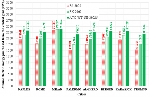
This graph shows that, for a given SWT model, the annual electric energy imported from the grid assumes the minimum value in the case of Palermo, while the maximum value is achieved for the city of Milan. For a given city, the annual electric energy purchased from the grid is minimum (1505.4 kWh) for the VASWT FS-2000, while it is maximum (2398.6 kWh) in the case of the HASWT ATO-WT-NE-300S5. For a given city and SWT model, the values reported in Figure 7 correspond to a relevant percentage of the annual building electricity demand (equal to 2408.96 kWh); this percentage varies between 62.5% (in Palermo) and 96.6% (in Milan) for the VASWT FS-2000, between 72.2% (in Palermo) and 98.7% (in Milan) for the HASWT FK-2000, and between 90.1% (in Palermo) and 99.6% (in Milan) for the HASWT ATO-WT-NE-300S5. These values indicate that the selected SWTs cover only a limited portion of the overall building electric consumption.
Figure 7. Annual electric energy purchased from the grid
In this paper the performance of the proposed scenarios where the building is served by both the SWTs and the central grid (as back-up) have been compared with those corresponding to a baseline scenario corresponding to the case where the electric demand of the same building is totally covered by the central grid only (without the SWTs). This comparison has been performed with the aim of determining the potential benefits in terms of electric energy imported from the grid (Section 4.1), equivalent global CO2 emissions (Section 4.2) and operating costs (Section 4.3); the simple payback period has been also calculated (Section 4.3).
4.1 Energy comparison
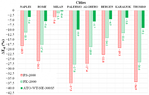
The percentage difference $\Delta \mathrm{E}_{\mathrm{el}}$ between the values of annual electric energy imported from the grid $E_{{el,imp }}^{P S}$ in the cases of the proposed scenarios (including the SWTs) with respect to the case of the reference scenario (without the SWTs) $E_{e l, i m p}^{R S}$ has been calculated according to the following formula:
$\Delta \mathrm{E}_{\mathrm{el}}=\frac{\mathrm{E}_{\mathrm{el}, \mathrm{imp}}^{\mathrm{PS}}-\mathrm{E}_{\mathrm{el}, \mathrm{imp}}^{\mathrm{RS}}}{\mathrm{E}_{\mathrm{el}, \mathrm{imp}}^{\mathrm{RS}}}$ (1)
Figure 8 reports the values of ΔEel as a function of both the wind turbine model and the city. All the values reported in this figure are negative; according to Eq. (1), this means that the proposed scenarios with the SWTs allow to reduce the electricity imported from the grid with respect to the reference scenario, whatever the wind turbine model and the city are. In greater detail, this figure indicates that, for a given city, the adoption of the SWTs allows to reduce the electric energy imported from the grid from a minimum of –0.4% in the case of the HASWT ATO-WT-NE-300S5 operating in Milan up to a maximum of –37.5% in the case of the VASWT FS-2000 operating in Palermo.
4.2 Environmental comparison
This work evaluated the environmental impacts by means of the energy output-based emission factor method proposed by Chicco and Mancarella [29]; it allows to estimate the global equivalent mass mx of a given pollutant x emitted while producing the energy output E according to the following formula:
$\mathrm{m}_{\mathrm{x}}=\mathrm{u}_{\mathrm{x}}^{\mathrm{E}} \cdot \mathrm{E}$ (2)
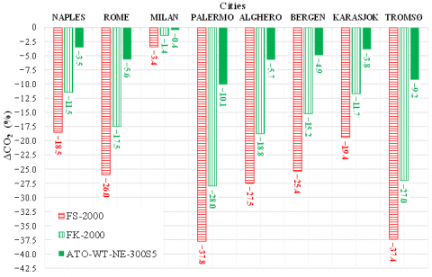
where, $u_x^E$ is the energy output-based emission factor of x per unit of E. CO2 emissions generally show to be quantitatively more significant than emissions of other pollutants. The CO2 emission factor associated to the electricity generation in Italy $u_{\mathrm{CO}_2}^{E_{\mathrm{el}}}$ depends on the location, the day of the year as well as the time of the day. According to the values suggested in the studies [30, 31], this factor ranges between 41.3 gCO2/kWhel and 827.3 gCO2/kWhel for the Italian cities and between 0 and 56.1 gCO2/kWhel for the Norwegian cities. The percentage difference $\Delta \mathrm{CO}_2$ between the values of global equivalent CO2 emissions in the case of the proposed scenarios (including the SWTs) with respect to the values of the reference scenario (without the SWTs) has been derived as follows:
$\Delta \mathrm{CO}_2=\frac{\mathrm{CO}_2^{\mathrm{PS}}-\mathrm{CO}_2^{\mathrm{RS}}}{\mathrm{CO}_2^{\mathrm{RS}}}=\frac{\sum_{\mathrm{i}} \mathrm{u}_{\mathrm{CO}_{2, \mathrm{i}}}^{\mathrm{E}_{\mathrm{el}}} \cdot \mathrm{P}_{\mathrm{el}, \mathrm{imp}, \mathrm{i}}^{\mathrm{PS}} \cdot \mathrm{STS}-\sum_{\mathrm{i}} \mathrm{u}_{\mathrm{CO}_{2, \mathrm{i}}}^{\mathrm{E}_{\mathrm{el}}} \cdot \mathrm{P}_{\mathrm{el}, \mathrm{imp}, \mathrm{i}}^{\mathrm{RS}} \cdot \mathrm{STS}}{\sum_{\mathrm{i}} \mathrm{u}_{\mathrm{CO}_{2, \mathrm{i}}}^{\mathrm{E}_{\mathrm{el}}} \cdot \mathrm{P}_{\mathrm{el}, \mathrm{imp}, \mathrm{i}}^{\mathrm{RS}} \cdot \mathrm{STS}}$ (3)
where, STS is the simulation time step (equal to 1 minute), and $u_{C O_{2, i}}^{E_{e l}}$ is the i-th CO2 emission factor associated to the i-th electric power imported from the grid in the case of the proposed scenario ($P_{e l, i m p, i}^{P S}$) or in the case of the reference scenario ($P_{e l, i m p, i}^{R S}$) at the same simulation time. Figure 9 underlines the results in terms of ΔCO2 upon varying both the city as well as the SWT model. The data are always negative and, therefore, the proposed scenarios including the SWTs allow to decrease the global equivalent CO2 emissions with respect to the reference scenario, whatever the city of the SWT model is. In more detail, this figure demonstrates that, for a given city, the utilization of the SWTs reduces the global equivalent CO2 emissions in comparison to the reference scenario from a minimum of –0.4% in the case of the HASWT ATO-WT-NE-300S5 in Milan up to a maximum of –37.8% associated to the VASWT FS-2000 in Palermo.
Figure 8. ΔEel upon varying the SWT model and city
Figure 9. ΔCO2 upon varying the SWT model and city
4.3 Economic comparison
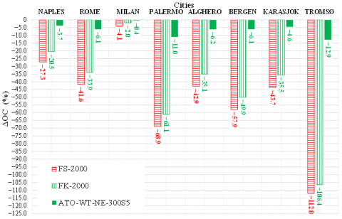
The percentage difference ΔOC between the values of operating costs (associated to the electricity imported from the grid) in the cases of the proposed scenarios (including the SWTs) with respect to the values of operating costs OCRS of the reference scenario (without the SWTs) has been calculated via this formula:
$\Delta \mathrm{OC}=\frac{\left(\mathrm{OC}^{\mathrm{PS}}-\mathrm{REV}_{\mathrm{el}, \text { sold }}\right)-\mathrm{OC}^{\mathrm{RS}}}{\mathrm{OC}^{\mathrm{RS}}}=\frac{\sum_{\mathrm{i}}\left(\mathrm{UC}_{\mathrm{el}, \mathrm{imp}, \mathrm{i}} \cdot \mathrm{P}_{\mathrm{el}, \mathrm{imp}, \mathrm{i}}^{\mathrm{PS}}-\mathrm{UC}_{\mathrm{el}, \text { sold }, \mathrm{i}} \cdot \mathrm{P}_{\mathrm{el}, \text { sold }, \mathrm{i}}^{\mathrm{PS}}\right)-\sum_{\mathrm{i}} \mathrm{UC}_{\mathrm{el}, \mathrm{imp}, \mathrm{i}} \cdot \mathrm{P}_{\mathrm{el}, \mathrm{imp}, \mathrm{i}}^{\mathrm{RS}}}{\sum_{\mathrm{i}} \mathrm{UC}_{\mathrm{el}, \mathrm{imp}, \mathrm{i}} \cdot \mathrm{P}_{\mathrm{el}, \mathrm{imp}, \mathrm{i}}^{\mathrm{RS}}}$ (4)
where, REVel,sold is the annual revenue obtained thanks to the electric energy sold to the grid, UCel,sold,i and UCel,imp,i are, respectively, the unit price of electric energy sold to the grid and the unit cost of electric energy imported from the grid. In the case of the Italian cities, the values of UCel,imp,i have been obtained according to the values indicated in the study [32] by considering the zone of Italy where the city is located (Central-South, North, Sicily, Sardinia). With reference to Norwegian cities, the values of UCel,imp,i have been defined according to those suggested by the federation of the European electricity industry based on the zone of Norway (Norway_4 and Norway_5) [33] where the considered cities are located. The values of UCel,sold,i for the selected Italian cities has been adopted according to the study [34]. In the cases of the Norwegian cities, the unit price of electricity sold to the grid UCel,sold,i has been assumed equivalent to the unit cost of electricity purchased from the grid UCel,imp,i when the electrical energy production exceeds the demand of the individual residential building [35]. According to studies [32-35], the maximum UCel,imp,i and UCel,sold,i for the Italian cities is equal to 400 €/MWh and 170 €/MWh, respectively, while for the Norwegian cities they are both equal to 332 €/MWh. Figure 10 shows the results in terms of $\Delta$OC upon varying both the city and the SWT model. This figure reports only negative values (whatever the city or the SWT model is), so the proposed scenarios with the SWTs always allow to decrease the operating costs in comparison with the reference scenario. In further detail, this plot underlines that, for a given city, the utilization of the SWTs decreases the operating costs in comparison to the reference scenario from a minimum of –0.4% in the case of the HASWT ATO-WT-NE-300S5 operating in Milan up to a maximum of –112.0% in the case of the VASWT FS-2000 operating in Tromsø.
The utilization of SWTs require a larger investment cost in comparison to the reference scenario. The simple payback period (SPB) represents the period that is needed to recover the extra investment thanks to both the savings in terms of operating costs as well as the revenues corresponding to the electricity sold to the grid; it can be obtained as follows:
$\mathrm{SPB}=\frac{\mathrm{WT}^{\mathrm{CC}}}{\left(\mathrm{OC}^{\mathrm{PS}}-\mathrm{OC}^{\mathrm{RS}}\right)+\mathrm{REV}_{\mathrm{el}, \text { sold }}}$ (5)
where, WTCC is the capital cost of SWTs.
Figure 10. ΔOC upon varying the SWT model and city
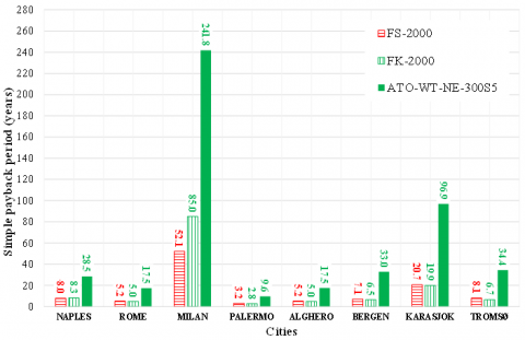
Figure 11 reports the values of SPB upon varying both the city and the SWT model. This plot highlights that SPB ranges from a minimum of 2.8 years (obtained when the HASWT FK-2000 operates in Palermo) up to a maximum of 241.8 years (that is achieved for the HASWT ATO-WT-NE-300S5 installed in Milan). The HASWT FK-2000 and the VASWT FS-2000 are characterized by similar SPBs, that can be assumed as suitable from an economic point of view (except in the case of Milan) taking into account that the expected SWTs lifetime is about 20÷25 years; the HASWT ATO-WT-NE-300S5 is characterized by much larger SPBs in contrast to the other SWTs, with acceptable values only when it is installed in Palermo, Rome and Alghero.
Figure 11. SPB upon varying the SWT model and city
In this study, the performance of a VASWT (model FS-2000 [13] with power output of 2100 W at 12 m/s and rotor swept area equal of 1.60 m2) have been assessed and compared with those of both a HASWT (model FK-2000 [14] with power output of 2100 W at 12 m/s and rotor swept area of 6.15 m2) and a HASWT (model ATO-WT-NE-300S5 [15] with power output of 307 W at 12 m/s and rotor swept area of 1.43 m2) while serving a typical single-family house. The analyses have been performed via the software TRNSYS [19] upon varying the city of installation considering 5 Italian and 3 Norwegian cities. The simulations indicated that, whatever the SWT model and the city are, the SWTs reduce the electric energy imported from the grid, the global equivalent CO2 emissions and the operating costs up to about –37.5%, –37.8% and –112.0%, respectively. In particular, the best results have been obtained in the case of the VASWT FS-2000 operating in Palermo, while the worst data have been achieved with reference to the HASWT ATO-WT-NE-300S5 operating in Milan. The results showed that, for a given SWT model, climatic conditions strongly affect the performance, with electricity generation in Palermo between 19.8 and 33.7 times larger than those associated to Milan. In addition, the simulations highlighted that, for a given city, the VASWT FS-2000 can increase the generated electricity by a minimum of 1.05 times (in Tromsø) up to a maximum of 1.80 times (in Milan) in comparison to the HASWT FK-2000, together with a reduced size; with respect to the HASWT ATO-WT-NE-300S5, the VASWT FS-2000 occupies a larger volume, but it can strongly enhance the electricity generation by a minimum of 8.47 times (in Palermo) up to a maximum of 11.54 times (in Milan). The HASWT FK-2000 and the VASWT FS-2000 showed similar simple payback periods, fully suitable from an economic point of view (except in the case of Milan); the shortest SPB (2.8 years) was associated to the HASWT FK-2000 operating in Palermo; the data demonstrated that the HASWT ATO-WT-NE-300S5 is characterized by acceptable SPBs only in the case of Palermo, Rome and Alghero.
[1] United Nations Environment Programme. (2025). Global Status Report for Buildings and Construction 2024/2025. https://www.unep.org/resources/report/global-status-report-buildings-and-construction-20242025.
[2] Chong, W.T., Muzammil, W.K., Wong, K.H., Wang, C.T., Gwani, M., Chu, Y.J., Poh, S.C. (2017). Cross axis wind turbine: Pushing the limit of wind turbine technology with complementary design. Applied Energy, 207: 78-95. https://doi.org/10.1016/j.apenergy.2017.06.099
[3] Yang, A.S., Su, Y.M., Wen, C.Y., Juan, Y.H., Wang, W.S., Cheng, C.H. (2016). Estimation of wind power generation in dense urban area. Applied Energy, 171: 213-230. https://doi.org/10.1016/j.apenergy.2016.03.007
[4] Ying, P., Chen, Y.K., Xu, Y.G., Tian, Y. (2015). Computational and experimental investigations of an omni-flow wind turbine. Applied Energy, 146: 74-83. https://doi.org/10.1016/j.apenergy.2015.01.067
[5] Weekes, S.M., Tomlin, A.S., Vosper, S.B., Skea, A.K., Gallani, M.L., Standen, J.J. (2015). Long-term wind resource assessment for small and medium-scale turbines using operational forecast data and measure–correlate–predict. Renewable Energy, 81: 760-769. https://doi.org/10.1016/j.renene.2015.03.066
[6] IEC, IEC. 61400-2. Wind Turbines-Part 2: Small Wind Turbines. IEC: Geneva, Switzerland, 2013. https://webstore.iec.ch/en/publication/5433.
[7] Calautit, K., Johnstone, C. (2023). State-of-the-art review of micro to small-scale wind energy harvesting technologies for building integration. Energy Conversion and Management: X, 20: 100457. https://doi.org/10.1016/j.ecmx.2023.100457
[8] Anup, K.C., Whale, J., Urmee, T. (2019). Urban wind conditions and small wind turbines in the built environment: A review. Renewable Energy, 131: 268-283. https://doi.org/10.1016/j.renene.2018.07.050
[9] Tummala, A., Velamati, R.K., Sinha, D.K., Indraja, V., Krishna, V.H. (2016). A review on small scale wind turbines. Renewable and Sustainable Energy Reviews, 56: 1351-1371. https://doi.org/10.1016/j.rser.2015.12.027
[10] Rosato, A., Perrotta, A., Maffei, L. (2024). Commercial small-scale horizontal and vertical wind turbines: A comprehensive review of geometry, materials, costs and performance. Energies, 17(13): 3125. https://doi.org/10.3390/en17133125
[11] Mohit, S., Reddy, M.A., Karthik, K.V.P., Mohanta, A. (2023). Hybrid power system. International Journal for Research in Applied Science and Engineering Technology, 11: 509-537. https://doi.org/10.22214/ijraset.2023.50117
[12] Fadil, J., Ashari, M. (2017). Performance comparison of vertical axis and horizontal axis wind turbines to get optimum power output. In 2017 15th International Conference on Quality in Research (QiR): International Symposium on Electrical and Computer Engineering, Nusa Dua, Bali, Indonesia, pp. 429-433. https://doi.org/10.1109/QIR.2017.8168524
[13] FLTXNY, Wuxi Flyt New Energy Technology Co., Ltd., model FS-2000. https://www.flytpower.com/200w-2kw-12v-24v-48v-96v-vertical-wind-turbine-coreless-permanent-magnet-generator-for-home-use-2-product/.
[14] FLTXNY, Wuxi Flyt New Energy Technology Co., Ltd., model FK-2000: https://www.flytpower.com/fltxny-2kw-horizontal-wind-turbine-generator-48v-96v-120v-230v-with-2000w-grid-tie-mppt-inverter-bult-in-wifi-limiter-product/.
[15] ATO, model ATO-WT-NE-300S5. https://www.ato.com/300w-wind-turbine.
[16] Rosato, A., Perrotta, A., Maffei, L. (2024). Dynamic simulation of different vertical axis micro wind turbines serving a typical house in Italy: Assessment of energy, environmental and economic impacts. In E3S Web of Conferences, Nantes, France, p. 01004. https://doi.org/10.1051/e3sconf/202457201004
[17] Rosato, A., Perrotta, A., Maffei, L. (2024). Influence of building electric demands on performance of a vertical axis micro wind turbine in Italy: Energy, environmental and economic numerical assessment. Journal Européen des Systèmes Automatisés, 57(6): 1639-1647. https://doi.org/10.18280/jesa.570611
[18] Rosato, A., Perrotta, A., Maffei, L. (2025). Effects of different wind speed databases on the performance of a vertical axis micro wind turbine integrated with a typical residential house: A comparative simulation analysis for five Italian cities. Building Simulation Applications BSA 2024, 1(1): 469-477. https://doi.org/10.13124/9788860462022
[19] A Transient Systems Simulation Program. Solar Energy Laboratory, University of Wisconsin-Madison. https://sel.me.wisc.edu/trnsys/.
[20] McKenna, E., Thomson, M., Barton, J. (2015). CREST demand model. Loughborough University. https://doi.org/10.17028/rd.lboro.2001129.v8
[21] Rosato, A., Ciervo, A., Ciampi, G., Scorpio, M., Guarino, F., Sibilio, S. (2020). Energy, environmental and economic dynamic assessment of a solar hybrid heating network operating with a seasonal thermal energy storage serving an Italian small-scale residential district: Influence of solar and back-up technologies. Thermal Science and Engineering Progress, 19: 100591. https://doi.org/10.1016/j.tsep.2020.100591
[22] Sibilio, S., Ciampi, G., Rosato, A., Entchev, E., Yaici, W. (2016). Parametric analysis of a solar heating and cooling system for an Italian multi-family house. International Journal of Heat and Technology, 34(S2): S458-464. https://doi.org/10.18280/ijht.34S238
[23] Rosato, A., Guarino, F., Sibilio, S., Entchev, E., Masullo, M., Maffei, L. (2021). Healthy and faulty experimental performance of a typical HVAC system under Italian climatic conditions: artificial neural network-based model and fault impact assessment. Energies, 14(17): 5362. https://doi.org/10.3390/en14175362
[24] Erdenedavaa, P., Rosato, A., Adiyabat, A., Akisawa, A., Sibilio, S., Ciervo, A. (2018). Model analysis of solar thermal system with the effect of dust deposition on the collectors. Energies, 11(7): 1795. https://doi.org/10.3390/en11071795
[25] Smith, K., Randall, G., Malcolm, D., Kelley, N., Smith, B. (2002). Evaluation of wind shear patterns at midwest wind energy facilities (No. NREL/CP-500-32492). National Renewable Energy Lab., Golden, CO (US).
[26] Le Fouest, S., Mulleners, K. (2024). Optimal blade pitch control for enhanced vertical-axis wind turbine performance. Nature Communications, 15(1): 2770. https://doi.org/10.1038/s41467-024-46988-0
[27] Lawson, M.J., Melvin, J., Anathan, S., Gruchalla, K.M., Rood, J.S., Sprague, M.A. (2019). Blade-resolved, single-turbine simulations under atmospheric flow. Golden, CO: National Renewable Energy Laboratory, NREL/TP-5000-72760. https://www.nrel.gov/docs/fy19osti/72760.pdf.
[28] Marion, W., Urban, K. (1997). User’s manual for TMY2s (Typical Meteorological Years) - Derived from the 1961-1990 national solar radiation data base. NREL/TP-463-7668. https://doi.org/10.2172/87130
[29] Chicco, G., Mancarella, P. (2008). Assessment of the greenhouse gas emissions from cogeneration and trigeneration systems. Part I: Models and indicators. Energy, 33(3): 410-417. https://doi.org/10.1016/j.energy.2007.10.006
[30] Electricity Maps. Italy. https://portal.electricitymaps.com/datasets/IT.
[31] Electricity Maps. Norway. https://portal.electricitymaps.com/datasets/NO.
[32] Gestore Mercati Energetici. PUN INDEX GME. https://gme.mercatoelettrico.org/en-us/Home/Results/Electricity/MGP/Results/PUN.
[33] Eurelectric Wholesale Electricity Price. https://electricity-data.eurelectric.org/electricity-price.html.
[34] Terna, S.P.A. (2025). Monthly Report on Electricity System March 2025. https://download.terna.it/terna/Monthly%20Report%20on%20the%20Electricity%20System_march_25_EN_8dd8cb341b40f6c.pdf.
[35] Haugaland Kraft. https://hkraft.no/produkter/strom/vare-stromavtaler/solkraft-stromavtale/.