Nouressadate Merzouka*![]() | Mohamed Ladjal
| Mohamed Ladjal![]() | Abdesslam Belaout
| Abdesslam Belaout![]() | Slimane Medjmadj
| Slimane Medjmadj![]()
© 2025 The authors. This article is published by IIETA and is licensed under the CC BY 4.0 license (http://creativecommons.org/licenses/by/4.0/).
OPEN ACCESS
Accurate modeling of photovoltaic (PV) systems is essential for performance optimization and fault diagnosis, yet is challenged by their nonlinear dynamics and dependency on environmental conditions and health status. This paper introduces a black-box, state-space identification approach that employs a bidirectional long short-term memory (BiLSTM) network. We frame the I-V curve modeling as a sequence-to-sequence task, where the BiLSTM predicts the current sequence (I) from a voltage sweep (V) and contextual inputs (irradiance, temperature, fault state). Trained on a comprehensive simulated dataset covering diverse operational and fault scenarios, the model demonstrates excellent performance, achieving a determination coefficient (R²) of over 0.99, alongside a minimal Root Mean Square Error (RMSE). Crucially, the model accurately predicts not only the I-V curve shape but also its key physical parameters (Pmax, Vmpp, Voc, Isc), validating the physical relevance of the learned representation. This study confirms that a BiLSTM can create a robust and accurate "digital twin" of a PV system, offering a powerful data-driven alternative to traditional physics-based models, especially for real-time monitoring and diagnostic applications.
BiLSTM, black-box modeling, photovoltaic system, recurrent neural networks, state-space modeling, surrogate model, system identification
As photovoltaic (PV) systems become increasingly central to the global energy transition, ensuring they operate efficiently and reliably is a top priority. We need accurate models to maximize the power output of these systems, identify faults before they become serious problems, and employ more intelligent control methods. Yet, building these models is not straightforward. A PV system's performance is complex and nonlinear, changing with factors like solar irradiance (G), temperature (T), and its physical condition. Traditional physics-based approaches, such as the single-diode model, often fail to provide accurate results. Their parameters are difficult to pin down, and they struggle to replicate the system's full dynamic behavior. This is where black-box system identification offers a practical solution. It enables us to build models directly from input-output data, without requiring an understanding of the complex physics within [1].
Deep learning provides the right tools for this challenge. Recurrent neural networks (RNNs), for example, are excellent for approximating nonlinear dynamic systems because they are specifically designed to process sequential data [2]. In recent years, Transformer models have become a key tool for working with sequential data. This is because they are very good at finding complex connections between data points that are far apart, an area where they often outperform traditional RNNs [3]. Researchers have successfully used them for specific PV tasks, like predicting the maximum power point or forecasting short-term power output [4, 5]. The field is also advancing with new designs like Mamba, which cleverly combines state-space ideas to be more efficient [6]. However, one major drawback is that these models typically require very large amounts of data to learn properly. For our work on I-V curve modeling, we are using a well-structured but moderately sized dataset. In this situation, we found that a recurrent model like the BiLSTM is still a very practical and effective choice. Within this context of neural network modeling for PV systems, research has largely followed two distinct paths. The most common path involves input-output models, which have been primarily applied to two tasks. For power output forecasting, numerous studies have demonstrated the effectiveness of hybrid architectures, such as CNN-LSTMs [7-9]. For static I-V curve characterization, other works use ANNs or neuro-fuzzy systems to estimate key electrical parameters for applications like MPPT optimization [10, 11]. The main drawback of these input-output models is their narrow focus. While successful in forecasting, their utility is restricted because they only describe a single output or a static state. They therefore fail to capture the system's internal dynamics, which limits their application in physical analysis and diagnostics.
In contrast, the state-space framework provides a more structured and powerful representation. Foundational work established the advantages of using neural networks within this framework, highlighting benefits like model parsimony and applicability to robust control [12, 13], and recent advances with deep learning have revitalized its use. What makes the state-space approach so powerful is that it tries to understand how the system works on the inside, instead of just memorizing the relationship between inputs and outputs. A major 2024 survey by Pillonetto et al. [14] points out that because these models learn the internal dynamics, they are much better at generalizing to new situations and are more reliable for simulations. On top of that, work by Gedon et al. [15] shows that deep state-space models are built to track complex patterns over long periods, which is something simpler input-output models often struggle with. This is a hot topic in research right now, with ongoing work focused on making these models even better for tricky, real-world systems with noise and uncertainty [16]. Even within physics-based modeling of PV systems, a state-space formulation is considered essential for capturing full dynamic behaviors [17]. Despite these parallel advances, a critical gap persists in the literature: few studies apply a data-driven state-space formalism to identify the complete I-V curve of a PV system, and even fewer validate the physical relevance of the learned state representation.
Our work aims to fill this gap. We introduce a method for data-driven state-space identification that uses a bidirectional long short-term memory (BiLSTM) network to model the entire current-voltage (I-V) curve as a dynamic sequence. We frame this as a sequence-to-sequence task where the network learns to predict the current sequence (I) from a voltage sweep (V) and its context (G, T, fault state). The network's internal hidden state serves as an estimator of the unobservable physical state, implicitly learning the system's underlying functions. The key contribution here is proving that this learned representation is physically meaningful. We demonstrate this by successfully extracting key electrical parameters (Pmax, Vmpp, Voc, Isc) from the model's predicted I-V curves. In doing so, we create a robust and interpretable surrogate model—a true "digital twin" of the PV system.
Specifically, this paper contributes the following:
A new way to model the PV I-V curve using a state-space framework solved by a bidirectional RNN.
Proof that the network's hidden state learns a physically relevant representation of the system.
Validation of this concept by accurately extracting derived electrical parameters.
The rest of this paper is organized to walk through our research process and findings. Section II is dedicated to our complete methodology, covering everything from the state-space formulation to the model's architecture and training protocol. In Section III, we present the experimental results, beginning with the final model configuration and its training convergence, before moving on to a complete evaluation of its performance and a detailed analysis of the learned dynamics. Sections IV and V then provide a deeper discussion of these results, where we compare our state-space model against a static input-output approach and further validate its physical relevance by checking it against experimental dynamic behavior. Finally, Section VI concludes the paper with a summary of our contributions and suggests directions for future work.
In this section, we outline the proposed methodology for identifying photovoltaic systems. Our approach leverages the state-space theoretical framework to model the nonlinear internal dynamics of the system. We use bidirectional long short-term memory (BiLSTM) network to learn this model directly from the data. We first present the theoretical formulation of the problem and then describe its practical application to modeling the current-voltage (I-V) curve as a sequence-to-sequence regression task.
2.1 State-space modeling for dynamic systems
An effective model of a photovoltaic (PV) system must accomplish two key tasks: capture the immediate input-output response and account for the system's internal dynamics. Traditional approaches usually handle the first part well but struggle with the second. When these methods treat the system as a "black box," they typically only learn the direct mapping from input to output [1]. This approach, however, fundamentally limits their power, as they cannot model complex physical processes or yield genuinely interpretable results. For this reason, we adopt the state-space model, a more powerful representation that has proven superior for nonlinear system identification in terms of both parsimony and performance [12, 13]. This framework describes the system's evolution through two fundamental discrete-time equations:
State Transition Equation:
$x(k+1)=f(x(k), u(k))$ (1)
Observation Equation:
$y(k)=g(x(k), u(k))$ (2)
here, x(k)∈ℝⁿ is the unobservable state vector (where n is the state dimension), u(k)∈ ℝᵐ is the input vector (where m is the number of inputs), and y(k)∈ℝᵖ is the measured output vector (where p is the number of outputs). The state vector x(k) encapsulates all necessary information about the system's past to predict its future, making this framework particularly suitable for modeling complex dynamic systems. The functions f and g are the nonlinear mappings we seek to identify. The state-space framework has seen a revival with modern deep learning techniques [14], with recent studies exploring advanced methods such as stochastic RNNs [16], autoencoders [18], and models for complex switching systems [19]. While some research in the PV field has focused on physics-based state-space models [17], our approach leverages this powerful formalism in a data-driven manner, employing recurrent neural networks to learn the underlying nonlinear functions f and g directly from operational data.
2.2 Experimental setup and data acquisition
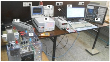
The dataset used in this study was generated using a real-time power electronics emulator of a photovoltaic array (PVA). This emulator, developed at the LEPCI laboratory (University of Sétif 1, Algeria), provides a high-fidelity environment for generating I-V characteristics under a wide range of precisely controlled conditions. The creation and performance evaluation of the emulator are thoroughly explained by Belaout et al. [20]. The core of the emulator illustrated in Figure 1 is a detailed electrical model of a PV array, designed in MATLAB/Simulink and deployed on a dSPACE DS1104 real-time control board. The simulated PVA consists of six series-connected photovoltaic modules, with each module comprising 36 solar cells based on the Bishop model, as detailed by Belaout et al. [21] and Belaout [22]. A rich and varied dataset was essential for this study. To achieve this, the emulator was used to systematically alter environmental conditions and introduce a range of fault types. This process generated data for one healthy state and five major fault categories, which were further broken down by severity and pattern to create a total of 22 distinct operational classes [21, 22]. To ensure data diversity, each class was generated with approximately 130 unique I-V curves by systematically varying environmental conditions, leading to a total database of nearly 2860 samples. The operational conditions and fault scenarios are detailed as follows:
Healthy Condition (NF): Normal operation with irradiance (G) varied from 100 to 1000 W/m² and temperature (T) from 0℃ to 60℃.
- F1: Partial Shading: 9 different shading patterns were simulated, varying the number of shaded cells (25%, 50%, 75%) and the number of affected modules (one, two, or three).
- F2: Increased Series Resistance (ISR): 5 levels of severity were created by increasing the series resistance of one module by 1 Ω, 5 Ω, 10 Ω, 15 Ω, and 20 Ω.
- F3: Bypass Diode Short-Circuit: 1 scenario where a single bypass diode in the array is short-circuited.
- F4: Bypass Diode Impedance Fault: 5 scenarios where a bypass diode is modeled as a faulty impedance with resistance values of 1 Ω, 5 Ω, 10 Ω, 15 Ω, and 20 Ω.
- F5: PV Module Short-Circuit: 1 scenario where an entire module is short-circuited.
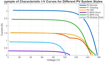
As the examples in Figure 2 demonstrate, each of the 22 unique operational states provides a distinct electrical signature based on its specific G and T conditions. It is this very diversity that forms the necessary empirical basis for training and validating the state-space model we propose.
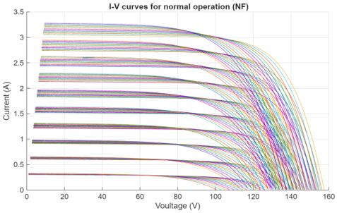
To illustrate the rich diversity of environmental conditions within each operational class, Figure 3 shows the complete set of 130 I-V curves generated for the Healthy Condition (NF) by systematically varying irradiance from 100 to 1000 W/m² and temperature from 0℃ to 60℃.
Figure 1. Photograph of the emulator used for data collection: 1) buck converters, 2) load, 3) programmable power source, 4) scope, 5) ControlDesk, 6) DS1104 platform [20]
Figure 2. Sample of characteristic I-V curves for different PV system states
Figure 3. Complete set of I-V curves for the normal operation (NF) class under varying environmental conditions
2.3 Data preprocessing and preparation
The raw data from the emulator, initially stored in 22 separate files corresponding to each operational state, was not immediately suitable for training. Therefore, a multi-step preparation pipeline was implemented. First, all separate files were consolidated into a single, unified dataset. Each sample in this dataset represents a full I-V curve and was then structured into a sequence-to-sequence format:
An input sequence, X, is a 4 × 130 matrix, since each I-V curve consists of N=130 points. The four rows correspond to the voltage sweep (V_k) and the contextual features: irradiance (G), temperature (T), and the fault type (D_encoded). These contextual features remain constant throughout the sequence.
A target sequence, Y, is a 1 × 130 vector containing the corresponding current values (I_k).
Next, to ensure an unbiased evaluation of the model's generalization ability, the entire dataset was randomly partitioned using a 70/30 split. 70% of the data was allocated to the training set, while the remaining 30% was set aside as a held-out test set. Finally, to improve training stability and efficiency, all features were normalized using Min-Max scaling, according to the formula:
${{x}_{-}}norm=\left( x-{{x}_{-}}min \right)/\left( {{x}_{-}}max-{{x}_{-}}min \right)$ (3)
Crucially, the normalization parameters (x_min and x_max) were calculated only on the training set and then applied to both the training and test sets. This prevents any data leakage from the test set into the training process. The resulting preprocessed data was then structured into cell arrays, the format required by MATLAB's Deep Learning Toolbox for training sequence-to-sequence models.
2.4 Bidirectional recurrent neural network architecture
To learn the nonlinear state-space functions f and g from sequential data, we selected a bidirectional recurrent neural network (Bi-RNN) as the core of our identification model. This choice is motivated by the inherent ability of RNNs to handle sequential information and the specific advantages of gated, bidirectional architectures for our problem, a practice that aligns with the state-of-the-art in modern data-driven system identification [14].
2.4.1 Long short-term memory (LSTM)
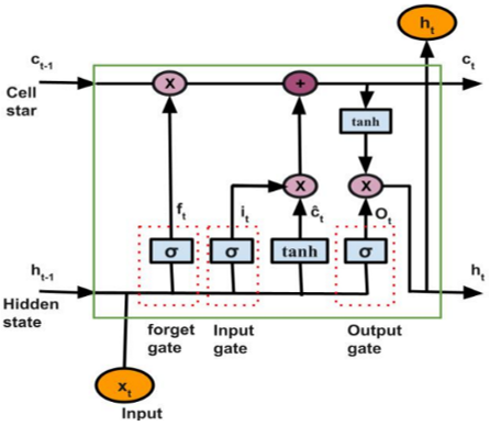
Our model is built using the long short-term memory (LSTM) cell, a sophisticated recurrent unit first introduced by Hochreiter and Schmidhuber [23]. Unlike a simple RNN unit, an LSTM cell incorporates a dedicated memory cell, c_t, which acts as a conveyor belt for information, and a series of gating mechanisms that precisely control the flow of this information. These gates allow the network to selectively add, remove, or expose parts of its memory [24], enabling it to capture dependencies over very long sequences [25]. This structure is particularly effective for learning state-space representations where the hidden state h(k) acts as an estimator of the physical state x(k) [15].
The core operations of an LSTM cell at a given time step t are governed by three main gates:
Forget Gate (f_t): This gate's role is to decide what to discard from the previous cell state, c_{t-1}. To do this, it processes the last hidden state, h_{t-1}, and the current input, x_t, to compute a value between 0 (forget everything) and 1 (keep everything).
$f_{-} t=\sigma\left(W_{-} f^*\left[h_{-}\{t-1\}, x_{-} t\right]+b_{-} f\right)$ (4)
Input Gate (i_t): This gate determines which new information to store in the cell state. It does this in two steps: a sigmoid layer selects which values to update, while a parallel tanh layer proposes a vector of new candidate values, c̃_t, to be added.
$i_{-} t=\sigma\left(W_{-} i^*\left[h_{-}\{t-1\}, x_{-} t\right]+b_{-} t\right)$ (5)
$\tilde{c}_{-} t=\tanh \left(W_{-} c *\left[h_{-}\{t-1\}, x_{-} t\right]+b_{-} c\right)$ (6)
The cell state is then updated by combining the forgotten past state with the new candidate information:
$c_{-} t=f_{-} t^{\circ} c_{-}\{t-1\}+i_{-} t^{\circ}{\check{c}}_{-} t$ (7)
Output Gate (o_t): This gate determines the next hidden state, h_t, which is a filtered version of the cell state. This is done in two steps: first, the cell state c_t is squashed through a tanh function, and then this result is multiplied element-wise by the output of the gate's sigmoid layer.
$o_{-} t=\sigma\left(W_{-} o *\left[h_{-}\{t-1\}, x_{-} t\right]+b_{-} o\right)$ (8)
$h_{-} t=o_{-} t^{\circ} \tanh \left(c_{-} t\right)$ (9)
In these equations, σ represents the sigmoid activation function, denotes the element-wise product, and W and b are the learnable weight matrices and bias vectors for each gate, respectively (see Figure 4).
Figure 4. The internal structure of a long short-term memory (LSTM) cell
2.4.2 The bidirectional architecture for complete contextual modeling
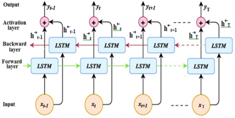
While a standard LSTM effectively captures past information, our system identification task requires a more holistic understanding of the entire I-V curve. To achieve this, we implement the LSTM cells within a Bidirectional LSTM (BiLSTM) framework. The BiLSTM is specifically designed for tasks where the full context of a sequence is important, drawing on the concept of bidirectionality first developed for RNNs and later LSTMs [26, 27]. As illustrated in Figure 5, the architecture achieves this by using two separate, parallel LSTM layers, each with an independent set of parameters, to process the input sequence from opposite directions:
Forward LSTM Layer: This layer processes the input sequence chronologically, from t=1 to N. At each step t, it calculates a forward hidden state $\mathrm{h}^{\rightarrow} \mathrm{t}$ which encodes information from the past (x_1, ..., x_t). This process can be abstractly represented as:
$\vec{h}_t=L S T M_{-} f w d\left(x_{-} t, \vec{h}_{t-1}\right)$ (10)
Backward LSTM Layer: To achieve a complete, 360-degree view of the sequence, the model needs information from the future as well as the past. This is the job of the backward LSTM layer, which processes the sequence in reverse to generate a hidden state $\mathrm{h}_{\mathrm{t}}^{\leftarrow}$ that summarizes the upcoming context (x_t, ..., x_N).
$\overleftarrow{h}_t=L S T M_{-} b w d\left(x_{-} t, \overleftarrow{h}_{t+1}\right)$ (11)
Combination of Outputs: To form a complete contextual representation, the outputs from both directions are combined at each time step. As shown in Figure 5, the most common and effective method, used in numerous applications, is to concatenate the forward and backward hidden states [28, 29]. This creates a final hidden state vector Ht that preserves all the information from both contexts:
$H_t=\left[\vec{h}_t ; \overleftarrow{h}_t\right]$ (12)
This concatenated vector Ht thus contains a rich representation of the input xt within the context of the entire sequence. This capability is particularly crucial for our system identification task. It allows the model to accurately reproduce the global shape of the I-V curve, including the complex distortions caused by conditions like partial shading [7, 8, 11], which a simple unidirectional model would struggle to capture. The ability to see the whole picture, therefore, makes the BiLSTM a significantly more powerful tool for creating a high-fidelity model of the PV system.
Figure 5. The internal structure of a bidirectional long short-term memory (BiLSTM) cell
2.5 Proposed model implementation
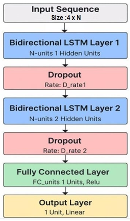
The architecture implemented in this work is a stacked BiLSTM network designed specifically for the sequence-to-sequence regression task. As visualized in Figure 6, the model is composed of layers, with key hyperparameters such as the number of hidden units and the dropout rate detailed in Table 1. The specific values for the structural hyperparameters were determined through the systematic optimization process described in the following sections.
Figure 6. The proposed stacked BiLSTM network architecture
2.6 Training and optimization protocol
To identify the best set of hyperparameters for our model, we performed a systematic search using the sample-efficient Bayesian optimization technique [30-32] instead of more common methods like grid or random search [33]. The search space included the number of BiLSTM hidden units, the dropout rate, the number of units in the fully connected layer, and the initial learning rate. The final model, using the optimal parameters found, was then trained with the Adam optimizer and an early stopping rule to prevent overfitting by halting the process if the validation loss stopped improving.
Table 1. Detailed description of the layers and key hyperparameters of the proposed BiLSTM model
|
Layer Type |
Key Hyper-Parameters |
Purpose |
|
Sequence Input Layer |
Input size |
Accepts the 4 × N input sequences |
|
Bilstm Layer |
N_units_1 hidden units |
Learns low-level temporal dependencies |
|
Dropout Layer |
Rate: D_rate_1 |
Regularization to prevent overfitting |
|
Bilstm Layer |
N_units_2 hidden units |
Learns high-level temporal features |
|
Dropout Layer |
Rate: D_rate_2 |
Further regularization |
|
Fully Connected Layer |
FC_units units |
Performs a final nonlinear transformation |
|
Relu Layer |
|
Introduces nonlinearity |
|
Fully Connected Layer |
unit, linear activation |
Maps features to a single scalar output (Î_k) for each time step |
|
Regression Layer |
|
Computes the mean squared Error loss for training |
2.7 Evaluation metrics
We wanted to answer two questions about our model's performance on the test data. First, how big are the prediction errors on average? We used the Root Mean Square Error (RMSE) to find that out. Second, how well do the model's predictions match the real data's spread? The R-squared (R²) value helped us answer that by showing how much of the real-world variation our model was able to capture. The equations for both are below:
$R M S E=\operatorname{sqrt}\left((1 / P) * \sum\left(I_{-} \text {real }-I_{-} \text {pred }\right)^2\right)$ (13)
where P is the total number of points across all test sequences.
$R^2=1-\left(\sum\left(I_{-} \text {real }-I_{-} \text {pred }\right)^2\right) / \sum\left(I_{-} \text {real }-I_{-} \text {mean}\right)^2$
Beyond these overall error metrics, we went further to check if our model made physical sense. To do this, we extracted key parameters like P_max, V_mpp, I_sc, and V_oc from both the predicted and the actual I-V curves. Comparing these values was a critical test to validate the physical relevance of our identified model.
In this section, we present the findings from our state-space identification performed using the proposed BiLSTM model. The model was trained with optimal hyperparameters determined by Bayesian optimisation, and the final training process achieved a validation RMSE of 0.0475 A.
Our analysis begins by illustrating the complexity of the identification challenge itself. A look at the I-V curves in Figure 2, which shows a sample from our test set, immediately reveals how dramatically the system's behaviour changes across its different operational and fault conditions. The system's state has a profound impact on the shape of the I-V curve. For example, under healthy conditions, the curve is typically smooth and concave. A fault like partial shading, however, can drastically alter this shape, introducing significant distortions and often creating multiple local power maxima. The true test for any system identification approach, therefore, is its ability to accurately model this full range of complex, nonlinear behaviors, rather than just fitting a single curve shape [34].
Following this, we will assess the model's overall predictive performance using global metrics and conclude with a detailed investigation into its physical relevance and learned internal dynamics.
3.1 Model configuration and training convergence
3.1.1 Optimal model parameters
We used a process to find the best model settings, which is described in the methodology.
The final choice was made based on one key factor: minimizing the error on the validation data. This method ensures a good balance between the model's ability to learn and the need to prevent overfitting, as detailed in Table 2.
Table 2. Final hyperparameters of the proposed BiLSTM model
|
Parameter |
Value |
Description |
|
Input Features |
4 |
V, G, T, Fault State |
|
BiLSTM Hidden Units |
140 per layer |
Number of hidden units in each of the two BiLSTM layers |
|
BiLSTM Layers |
2 (stacked) |
Number of stacked BiLSTM layers |
|
Fully Connected Units |
58 |
Number of units in the dense layer before the output |
|
Dropout Rate |
0.2225 |
Dropout rate applied after each BiLSTM layer |
|
Optimizer |
Adam |
Adaptive moment estimation optimizer |
|
Initial Learning Rate |
0.0026 |
Initial learning rate for the Adam optimizer |
|
Mini-batch Size |
32 |
Number of samples per training iteration |
|
Max Epochs |
100 |
Maximum number of training epochs |
|
Early Stopping Patience |
10 |
Number of epochs to wait for improvement before stopping |
3.1.2 Training convergence
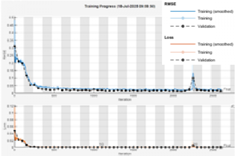
The training progress of the final model is shown in Figure 7. The plot shows how the Root Mean Square Error (RMSE) and the loss function changed during the training for both the training and validation sets.
At first, both the loss and RMSE dropped quickly, then the values became stable as the training continued. The process stopped automatically after 23 epochs because of the early stopping rule, which helped prevent the model from learning the training data too well (overfitting). This early stopping ensured that the model would perform well on new, unseen data. The final RMSE on the validation data at the point of convergence was 0.014278, showing that the training was successful and stable.
Figure 7. Training progress of the BiLSTM network
3.2 Overall identification performance
After training the model and confirming its convergence, we tested it with a separate set of 1630 I-V curves. The predictions were then converted back to their original units (Amperes). The model performed well and showed it could generalize to new data. The performance metrics on the test set were as follows:
Root Mean Square Error (RMSE): 0.0475 A
Coefficient of Determination (R²): 0.9974
The following figures further illustrate this high level of accuracy:
The correlation plot (Figure 8) compares predicted and actual current values. The data points form a very dense and narrow cluster around the y=x line, which represents an ideal prediction. This tight alignment visually confirms the model's robustness and its ability to make highly accurate predictions, consistent with the high R² score [35].
Figure 8. Correlation between predicted and actual values
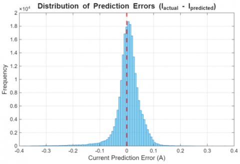
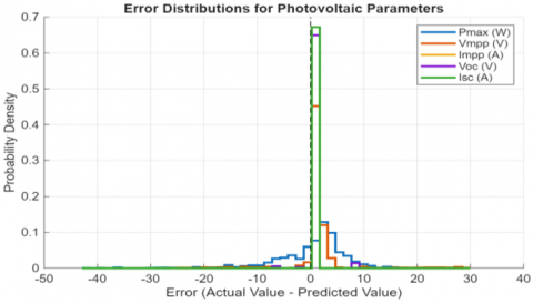
Figure 9. Distribution of prediction errors (I_{actual} - I_{predicted})
The error distribution histogram (Figure 9) provides further insight into the model's performance.
The distribution of prediction errors (I_actual - I_predicted) is sharply peaked and centered almost perfectly at zero, indicating that the model is unbiased and that the vast majority of errors are very close to zero. This narrow spread, with most errors falling within a ±0.1 A range, reinforces the reliability of the model and is consistent with the low overall RMSE.
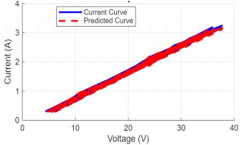
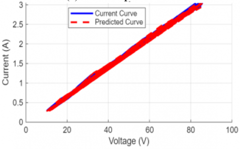
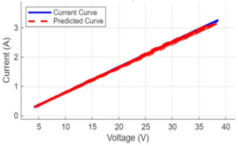
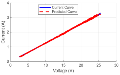
A visual check of the model's performance in Figure 10 confirms its high accuracy. Here, we've overlaid the predicted I-V curves on the actual curves for several random test samples. The two curves track each other very closely, even across different voltage and current ranges, which is a strong visual testament to the low RMSE and high R² scores [36].
(a) Test sample # 1323
(b) Test sample # 1524
(c) Test sample # 71
(d) Test sample # 317
Figure 10. Comparison of actual and predicted I-V curves for randomly selected test samples
3.3 Detailed analysis and validation of the identified state-space model
Despite the confirmation of the model's statistical accuracy through global metrics, additional analysis is essential to confirm that the model has grasped a valid state-space representation. To validate our identified state-space model beyond global metrics, we carry out a detailed, three-part analysis. First, we check how well the model follows a typical example of the system's behavior. Then, we take a closer look at the internal state dynamics and their physical meaning by using time-based plots and t-SNE visualizations. Finally, we test how well the model can predict critical physical parameters.
3.3.1 Dynamic identification performance
To visually assess the model's performance on a dynamic trajectory, a random sample from the test set was selected for detailed analysis. Figure 11 illustrates the identification process for this sample.
The figure's subplots show that (a) the model was subjected to a standard voltage sweep input. In response, (b) the model's predicted output ŷ(t) almost perfectly tracks the actual system output y(t), indicating a very high tracking accuracy. This is further confirmed in (c), where the prediction error e(t) remains small, stable, and centred around zero, demonstrating that the model's predictions are consistent and unbiased throughout the sequence.
Figure 11. Dynamic identification performance of the state-space model for a random test sample. Subplots show: (a) input voltage u(t); (b) comparison between actual y(t) and predicted ŷ(t) current; (c) prediction error e(t)
3.3.2 Analysis of the learned internal state
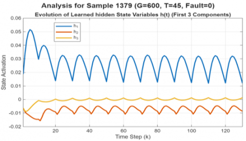
The main idea behind our state-space approach is that the hidden states of the BiLSTM can serve as estimators for the unobservable system state x(k).To check this, we first examined how the hidden states evolved for the same test sample (Figure 11). This analysis validates that the model has learned a coherent internal state-transition function.
$\mathrm{h}(k)=f(h(k-1), u(k))$.
This is the most insightful part of the analysis, as it shows how the first three components of the learned hidden state vector h(t) evolve. Figure 12 clearly shows that the hidden states don't change randomly. Instead, they follow a smooth and organized pattern that lines up perfectly with the input signal. What this tells us is that the network has successfully learned a stable and coherent set of internal rules—a transition function—which is precisely what a good state-space model should do.
Figure 12. Evolution of the first three components (h1, h2, h3) of the learned hidden state vector h(t) for the test sample shown in Figure 11
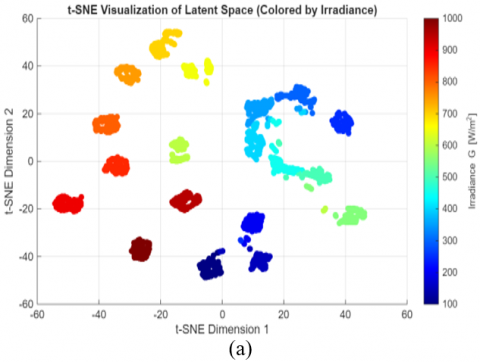
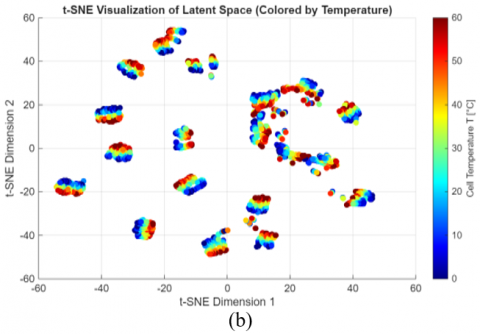
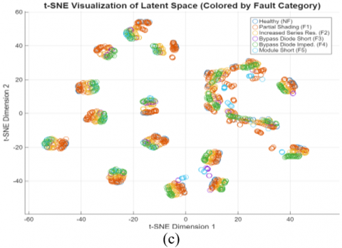
To further validate that this learned state is physically meaningful, we visualized the final hidden state h(t) for all test samples using the t-SNE technique. The results, presented in Figure 13, offer a direct visualization of the learned latent space.
The t-SNE visualizations provide a robust validation of our state-space approach, revealing that the model has learned to organize its latent space based on a clear physical hierarchy. The primary organizing factor is irradiance (a), followed by a secondary organization based on temperature (b) within each irradiance cluster, and a final, local organization based on fault categories (c), demonstrating that the model has learned to distinguish the unique dynamic signature of each health state. This automatically discovered structure confirms that the final hidden state h(t) is a physically meaningful embedding, not just a random vector. It demonstrates that our model has gone beyond simple curve-fitting to construct a true, interpretable internal state-space model of the PV system.
3.3.3 Physical parameter validation
This analysis provides strong evidence that the BiLSTM has successfully identified a meaningful internal state-space representation of the PV system. The learned hidden states are not arbitrary, but follow a clear dynamic structure, confirming that the model has learned an internal representation of the system's evolution, not just a static input-output mapping.
Now that we've seen that the model has learned a coherent internal dynamic, the next logical step is to check its practical usefulness. We did this by testing if it could accurately predict key physical parameters from the I-V curves. This test is essential because it confirms that our identified model is not just internally consistent but also physically meaningful.
Table 3. Performance on key physical parameter extraction
|
Parameter |
Mean Actual |
Mean Predicted |
Mean Absolute Error |
Relative Error (%) |
|
Pmax (W) |
146.96 |
147.1 |
0.13498 |
0.091849 |
|
Vmpp (V) |
88.54 |
88.032 |
0.50806 |
0.57382 |
|
Impp (A) |
2.1939 |
2.1908 |
0.003102 |
0.14141 |
|
Voc (V) |
81.917 |
81.828 |
0.088648 |
0.10822 |
|
Isc (A) |
0.2626 |
0.30619 |
0.04357 |
16.59 |
We extracted five standard PV parameters from both the predicted and the actual curves for all 1630 samples in the test set. Table 3 summarises the results, comparing the mean of the actual and predicted values and showing the resulting error metrics calculated on these means.
The results show a strong agreement for most parameters. The model predicts the mean maximum power (Pmax), maximum power point voltage (Vmpp), current (Impp), and open-circuit voltage (Voc) with relative errors on the mean of less than 1%. This high level of accuracy on derived physical quantities is strong evidence that the learned state-space representation is physically accurate.
A higher relative error of 16.6% was observed for the short-circuit current (Isc). However, as the error distribution analysis in Figure 14 reveals, this is not due to a model weakness but is primarily a statistical artefact. Looking at the error distribution for Isc, we see a tall, narrow peak right at zero. This shows two things: the model has no systematic bias, and its absolute errors are almost always tiny. The large percentage in the table is a direct result of the math involved, as the relative error formula exaggerates even these minor absolute errors when the actual Isc value is very low (≈0.26 A). This slight initial deviation can be attributed to a "sequence edge effect" occurring at the start of the voltage sweep (V ≈ 0), where the forward LSTM layer has less contextual information.
Figure 13. t-SNE visualization of the learned latent space, colored by (a) Irradiance (G), (b) Temperature (T), and (c) Fault category
Figure 14. Probability density functions of the prediction errors for each of the five extracted physical parameters
To get a more complete picture, we visualize the full error distributions for each parameter in Figure 14. In this visualization, we plot the probability density functions (PDFs) derived from the prediction errors, which lets us directly check for any model bias and see how consistent the predictions are.
The distributions in Figure 13 tell a clear story. All five are sharply peaked and centred on zero, a strong sign that our model is unbiased. Looking closer at Isc, its PDF is noticeably the most concentrated of the group. This confirms that the model's absolute performance for this specific parameter is, in fact, excellent. Nevertheless, the overall performance confirms that the model has acquired a physical understanding of the system, far beyond simple curve-fitting.
To understand the practical advantages of our state-space model, we needed a point of comparison. For this, we built and trained a standard static input-output model, a Multi-Layer Perceptron (MLP), on the same dataset. The MLP's role is to model the direct input-output relationship at each time step by treating each (V_k, I_k) point as an independent sample, using the same input features [V_k, G, T, Fault State] to predict the current I_k. To ensure a fair comparison, the MLP was designed with a comparable level of complexity and was trained under similar conditions as the BiLSTM model. The detailed architectural and training hyperparameters for the comparative MLP are presented in Table 4.
Table 4. Configuration of the comparative MLP model
|
Parameter |
Value |
|
Input Features |
4 |
|
Number of Hidden Layers |
2 |
|
Neurons per Hidden Layer |
128 |
|
Activation Function |
ReLU |
|
Output Layer |
1 Neuron (Linear) |
|
Optimizer |
Adam |
|
Initial Learning Rate |
0.001 |
|
Mini-batch Size |
32 |
The quantitative performance comparison of the two models on the test set is summarized in Table 5.
The data in Table 5 highlight the advantage of the state-space model. The BiLSTM achieves better results, shown by its lower RMSE and higher R² values, thanks to its capability to utilize the full sequential context of the data—an inherent limitation in static input-output models like the MLP. This qualitative difference in performance is further illustrated on representative test samples in Figure 15.
Table 5. Performance comparison between models
|
Model Type |
RMSE (A) |
R-Squared (R²) |
|
State-Space (BiLSTM) |
0.0475 |
0.9974 |
|
Input-Output (MLP) |
0.0815 |
0.9924 |
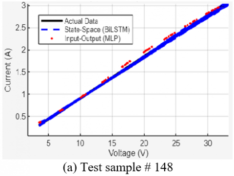
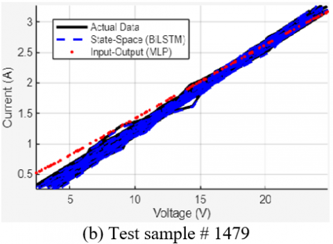
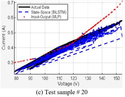
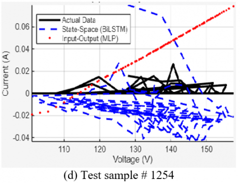
Figure 15. Qualitative comparison of the BiLSTM and MLP models on four representative test samples
On a clean I-V curve (Sample #148), the BiLSTM's prediction is nearly perfect, while the MLP shows slight deviations.
On a complex, noisy curve (Sample #1479), the BiLSTM successfully captures the subtle nonlinearities, whereas the MLP's prediction is overly linear and less accurate.
On a highly distorted curve under a severe fault (Sample #20), the MLP's predictions diverge completely, while the BiLSTM, though challenged, still manages to capture the overall trend.
On a low-current, erratic curve (Sample #1254), both models struggle, but the MLP produces a simple, incorrect linear trend, while the BiLSTM still attempts to model the complex, non-zero behavior of the data.
This comparison confirms that the state-space model (BiLSTM) is not only quantitatively more accurate but also qualitatively more robust. The key difference lies in the BiLSTM's use of sequential context, a capability that static input-output models lack by design, highlighting a fundamental advantage of the state-space approach [12, 13].
We can further validate the physical relevance of our identified state-space model by comparing its predictions with experimental results from the literature. For example, the work of Belaout [20] presents the dynamic response of a similar PV system's Maximum Power Point (MPP) to real-time changes in irradiance and temperature. Although our work focuses on static system identification, this comparison allows us to confirm that our model has learned the correct underlying physical behaviors.
5.1 Comparison of physical trends
The experimental data in the study [20] reveal two important physical trends. First, it shows a clear link between irradiance and current. When irradiance goes up, the maximum power point current (Impp) rises with it, leading to a direct increase in maximum power (Pmax). The second is the inverse relationship between temperature and voltage: as temperature increases, the maximum power point voltage (Vmpp) falls, slightly reducing Pmax.
What this means is that our model, despite being trained only on static I-V curves, has still learned these fundamental physical relationships. The highly accurate parameter predictions we show in Table 3 are strong evidence that our data-driven model has implicitly captured the correct dependencies between environmental conditions and key electrical parameters, and that these learned relationships align with the dynamic behavior seen in experiments.
5.2 Complementarity of the approaches
This comparison also highlights the collaboration between system identification and control algorithm validation. An MPPT algorithm, like the one tested in study [20], requires a target—the true Maximum Power Point—to track. Our work provides a direct method for predicting the location of this MPP under any given static condition.
Therefore, our identified BiLSTM model can be seen as a high-fidelity "virtual test bench" or surrogate model. It could be used to generate the reference I-V curves and target MPPs necessary for testing, validating, or even training new MPPT algorithms under thousands of simulated conditions. This task would be impractical to perform on a physical system.
This study introduced a state-space identification approach for modeling the nonlinear behavior of photovoltaic (PV) systems. We framed the I-V curve identification as a sequence-to-sequence task. We used a stacked bidirectional long short-term memory (BiLSTM) network to create a high-fidelity surrogate model. The proposed model achieved remarkable predictive accuracy, with a Coefficient of Determination (R²) exceeding 0.997 and a very low Root Mean Square Error (RMSE). This work has successfully shown that a state-space approach to I-V curve modeling can produce a physically relevant model that outperforms traditional static methods. The fundamental ability of our model to capture the system's internal dynamics is what allows it to make both highly accurate I-V curves and precise calculations of key electrical parameters like Pmax, Voc, and Vmpp. This capability is precisely what static models lack, which explains their poor performance when dealing with the complex dynamics of nonlinear fault conditions. Functioning as a "virtual test bench," it could be used to generate realistic I-V data for the development and validation of next-generation control algorithms, such as adaptive Maximum Power Point Tracking (MPPT) techniques. Furthermore, the model could be extended to predict long-term performance degradation by incorporating ageing effects into the training data. Validating this identification approach on data from a utility-scale, field-deployed PV plant is the critical next step to confirm its practical utility and scalability. Thus, a comparative analysis against state-of-the-art Transformer architectures would be a valuable future direction, especially on larger datasets.
What this work ultimately shows is that a data-driven approach can provide a robust and accurate alternative to traditional physics-based models for PV systems. This has important implications for the future of renewable energy, opening up new possibilities for real-time diagnostics, performance optimization, and the development of more intelligent control systems.
|
BiLSTM |
Bidirectional Long Short-Term Memory Network |
|
G |
Irradiance, W.m⁻² |
|
I-V |
Current-Voltage |
|
MLP |
Multilayer Perceptron |
|
PV |
Photovoltaic |
|
R2 |
Correlation Coefficient |
|
RMSE |
Root Mean Square Error |
|
RNN |
Recurrent Neural Networks |
|
T |
Temperature,℃ |
[1] Ayala, H.V.H., Habineza, D., Rakotondrabe, M., dos Santos Coelho, L. (2020). Nonlinear black-box system identification through coevolutionary algorithms and radial basis function artificial neural networks. Applied Soft Computing, 87: 105990. https://doi.org/10.1016/j.asoc.2019.105990
[2] Perrusquía, A., Yu, W. (2021). Identification and optimal control of nonlinear systems using recurrent neural networks and reinforcement learning: An overview. Neurocomputing, 438: 145-154. https://doi.org/10.1016/j.neucom.2021.01.096
[3] Jiang, H., Li, Q. (2023). Approximation rate of the transformer architecture for sequence modeling. Advances in Neural Information Processing Systems, 37: 68926-68955. https://doi.org/10.48550/arXiv.2305.18475
[4] Agrawal, P., Bansal, H.O., Gautam, A.R., Mahela, O.P., Khan, B. (2022). Transformer‐based time series prediction of the maximum power point for solar photovoltaic cells. Energy Science & Engineering, 10(9): 3397-3410. https://doi.org/10.1002/ese3.1226
[5] Scott, A., Sreedhara, S., Ayoola, F. (2025). Transformers applied to short-term solar PV power output forecasting. arXiv preprint arXiv: 2505.03188. https://doi.org/10.48550/arXiv.2505.03188
[6] Gu, A., Dao, T. (2023). Mamba: Linear-time sequence modeling with selective state spaces. arXiv preprint arXiv: 2312.00752. https://doi.org/10.48550/arXiv.2312.00752
[7] Boucetta, L.N., Amrane, Y., Chouder, A., Arezki, S., Kichou, S. (2024). Enhanced forecasting accuracy of a grid connected photovoltaic power plant: A novel approach using hybrid variational mode decomposition and a CNN LSTM model. Energies, 17(7): 1781. https://doi.org/10.3390/en17071781
[8] Sabri, M., El Hassouni, M. (2023). Predicting photovoltaic power generation using double-layer bidirectional long short-term memory–convolutional network. International Journal of Energy and Environmental Engineering, 14(3): 497-510. https://doi.org/10.1007/s40095-022-00530-4
[9] Chen, B., Lin, P., Lai, Y., Cheng, S., Chen, Z., Wu, L. (2020). Very-short-term power prediction for PV power plants using a simple and effective RCC-LSTM model based on short term multivariate historical datasets. Electronics, 9(2): 289. https://doi.org/10.3390/electronics9020289
[10] Amiri, A.F., Oudira, H., Chouder, A., Amiri, A.F. (2023). Prediction model of PV module based on artificial neural networks for the energy production. In Proc. 5th Novel Intelligent and Leading Emerging Sciences Conference (NILES), Giza, Egypt, pp. 85-88. https://doi.org/10.1109/NILES59815.2023.10296720
[11] Mohammed, H.A., Mohd-Mokhtar, R., Ali, H.I. (2025). An optimal adaptive neuro-fuzzy inference system for photovoltaic power system optimization under partial shading conditions. Energy Systems, 1-24. https://doi.org/10.1007/s12667-025-00745-4
[12] Rivals, I., Personnaz, L. (1996). Black-box modeling with state-space neural networks. Neural Adaptive Control Technology, World Scientific, pp. 237-264. https://doi.org/10.1142/9789812830388_0008
[13] Suykens, J.A.K., De Moor, B.L., Vandewalle, J. (1995). Nonlinear system identification using neural state space models, applicable to robust control design. International Journal of Control, 62(1): 129-152. https://doi.org/10.1080/00207179508921536
[14] Pillonetto, G., Aravkin, A., Gedon, D., Ljung, L., Ribeiro, A.H., Schön, T.B. (2025). Deep networks for system identification: A survey. Automatica, 171: 111907. https://doi.org/10.1016/j.automatica.2024.111907
[15] Gedon, D., Wahlström, N., Schön, T.B., Ljung, L. (2021). Deep state space models for nonlinear system identification. IFAC-PapersOnLine, 54(7): 481-486. https://doi.org/10.1016/j.ifacol.2021.08.406
[16] Liu, X., Du, X., Yang, X., Cai, C. (2023). Improved stochastic recurrent networks for nonlinear state space system identification. In IECON 2023-49th Annual Conference of the IEEE Industrial Electronics Society, Singapore, Singapore, pp. 1-6. https://doi.org/10.1109/IECON51785.2023.10311812
[17] Batzelis, E.I., Anagnostou, G., Cole, I.R., Betts, T.R., Pal, B.C. (2018). A state-space dynamic model for photovoltaic systems with full ancillary services support. IEEE Transactions on Sustainable Energy, 10(3): 1399-1409. https://doi.org/10.1109/TSTE.2018.2880082
[18] Yamada, K., Maruta, I., Fujimoto, K. (2023). Subspace state-space identification of nonlinear dynamical system using deep neural network with a bottleneck. IFAC-PapersOnLine, 56(1): 102-107. https://doi.org/10.1016/j.ifacol.2023.02.018
[19] Zhang, Y., Yu, C., Fabiani, F. (2025). Neural network-based identification of state-space switching nonlinear systems. arXiv preprint arXiv: 2503.10114. https://doi.org/10.48550/arXiv.2503.10114
[20] Belaout, A., Krim, F., Talbi, B., Feroura, H., et al. (2017). Development of real time emulator for control and diagnosis purpose of Photovoltaic Generator. In 2017 6th International Conference on Systems and Control (ICSC), Batna, Algeria, pp. 139-144. https://doi.org/10.1109/ICoSC.2017.7958653
[21] Belaout, A., Krim, F., Mellit, A., Talbi, B., Arabi, A. (2018). Multiclass adaptive neuro-fuzzy classifier and feature selection techniques for photovoltaic array fault detection and classification. Renewable Energy, 127: 548-558. https://doi.org/10.1016/j.renene.2018.05.008
[22] Belaout, A. (2018). Application of artificial intelligence techniques for faults diagnosis in photovoltaic systems. Doctoral dissertation. Ferhat Abbas Sétif 1 University, Sétif, Algeria.
[23] Hochreiter, S., Schmidhuber, J. (1997). Long short-term memory. Neural Computation, 9(8): 1735-1780. https://doi.org/10.1162/neco.1997.9.8.1735
[24] Gers, F.A., Schmidhuber, J., Cummins, F. (2000). Learning to forget: Continual prediction with LSTM. Neural Computation, 12(10): 2451-2471. https://doi.org/10.1162/089976600300015015
[25] Landi, F., Cornia, M., Baraldi, L., Cucchiara, R. (2021). Working Memory Connections for LSTM. Neural Networks, 144: 334-341. https://doi.org/10.1016/j.neunet.2021.08.030
[26] Graves, A., Schmidhuber, J. (2005). Framewise phoneme classification with bidirectional LSTM networks. In Proceedings 2005 IEEE International Joint Conference on Neural Networks, Montreal, QC, Canada, pp. 2047-2052. https://doi.org/10.1109/IJCNN.2005.1556215
[27] Mienye, I.D., Swart, T.G. (2024). A comprehensive review of deep learning: Architectures, recent advances, and applications. Information, 15(12): 755. https://doi.org/10.3390/info15120755
[28] Li, R., Zhang, X., Dai, H., Zhou, B., Wang, Z. (2019). Interpretability analysis of heartbeat classification based on heartbeat activity’s global sequence features and BiLSTM-attention neural network. IEEE Access, 7: 109870-109883. https://doi.org/10.1109/ACCESS.2019.2935471
[29] Aamir, M., Bhatti, M.A., Bazai, S.U., Marjan, S., et al. (2022). Predicting the environmental change of carbon emission patterns in South Asia: A deep learning approach using BiLSTM. Atmosphere, 13(12): 2011. https://doi.org/10.3390/atmos13122011
[30] Snoek, J., Larochelle, H., Adams, R.P. (2012). Practical bayesian optimization of machine learning algorithms. Advances in Neural Information Processing Systems, 25: 2951-2959.
[31] Shahriari, B., Swersky, K., Wang, Z., Adams, R.P., De Freitas, N. (2015). Taking the human out of the loop: A review of Bayesian optimization. Proceedings of the IEEE, 104(1): 148-175. https://doi.org/10.1109/JPROC.2015.2494218
[32] Wu, J., Chen, X.Y., Zhang, H., Xiong, L.D., Lei, H., Deng, S.H. (2019). Hyperparameter optimization for machine learning models based on Bayesian optimization. Journal of Electronic Science and Technology, 17(1): 26-40. https://doi.org/10.11989/JEST.1674-862X.707157
[33] Bergstra, J., Bengio, Y. (2012). Random search for hyper-parameter optimization. The Journal of Machine Learning Research, 13(1): 281-305. https://dl.acm.org/doi/abs/10.5555/2188385.2188395
[34] Liu, S., Hao, X., Meng, Z., Li, J., Cui, T., Wei, L. (2021). Application of SRNN-GRU in Photovoltaic power Forecasting. In E3S Web of Conferences, pp. 02001. https://doi.org/10.1051/e3sconf/202125602001
[35] Gheisari, M., Ebrahimzadeh, F., Rahimi, M., Moazzamigodarzi, M., et al. (2024). Deep learning: Applications, architectures, models, tools, and frameworks: A comprehensive survey. CAAI Transactions on Intelligent Technology, 9(5): 835-862. https://doi.org/10.1049/cit2.12180
[36] Jia, C., Chen, F., Xiang, L., Lan, W., Feng, G. (2022). When distributed formation control is feasible under hard constraints on energy and time?. Automatica, 135: 109984. https://doi.org/10.1016/j.automatica.2021.109984