Fifin Sonata*![]() | Azlan
| Azlan![]() | Andy Sapta
| Andy Sapta![]() | Yuli Panca Asmara
| Yuli Panca Asmara![]() | Aeri Rachmad
| Aeri Rachmad![]()
© 2025 The authors. This article is published by IIETA and is licensed under the CC BY 4.0 license (http://creativecommons.org/licenses/by/4.0/).
OPEN ACCESS
With the rapid pace of industrial growth, the demand for optimized scheduling has become increasingly critical. Scheduling is the activity of allocating limited resources to perform a few jobs. The purpose of this study is to build an optimization model in solving the flow shop production machine scheduling by minimizing 2 objects, namely makespan and total tardiness. Optimization of these two objects is an opposite optimization. The method used is the Non-Dominated Sorting Genetic Algorithm for multi-objective optimization: NSGA-II algorithm which can integrate the problems of 2 objects. This algorithm is developed into an optimization form to see the value of the solution. The developed model will provide a flow shop production machine scheduling solution in the form of a Pareto optimal solution that can provide a set of alternative solutions for decision makers in making production machine scheduling. To see the value of the solution, a comparison of the dominance of the Aggregate of Function (AOF) solution with the NSGA-II solution is carried out. The Pareto-optimal solution produced by NSGA-II successfully dominates 100% of the AOF solution. Similarly, a comparison of NSGA-II solutions with AOF solutions shows that the population of Pareto-optimal NSGA-II solutions is better, successfully dominating 100% of the AOF solutions. Thus, all Pareto-optimal solutions are equally good.
model, multi-objective, NSGA-II, optimization, production machine scheduling
Production machine scheduling in the industrial world, whether in manufacturing, production, or agro-industry, plays a crucial role in decision-making [1]. Companies strive to achieve the most effective and efficient scheduling to increase productivity while minimizing total cost and time [2]. One model that can be applied to made-to-order manufacturing environments is the flow shop scheduling model [3]. Production machine scheduling problems typically involve the arrangement and management of jobs to be processed on a series of machines. One of the difficulties in arranging and managing jobs across available machines is the difficulty of finding appropriate techniques to create an optimal production machine scheduling model that meets all established scheduling criteria.
The scheduling model developed in this study currently assumes ideal conditions where all machines are continuously available and each worker has homogeneous skills. To improve the practicality and robustness of the solution, sensitivity analysis and robustness testing are recommended. Sensitivity analysis can be performed by varying critical parameters, such as machine processing time, breakdown probability, or worker productivity, and then evaluating the changes in objectives, such as makespan or total tardiness.
In addition, robustness testing can be performed through Monte Carlo simulations incorporating random distributions on critical variables, or through robust optimization methods, where the optimization objective is expanded to minimize the worst-case impact of disruptions. In this way, the solution is not only nominally optimal but also robust to uncertainty, thus providing a clear trade-off between efficiency (makespan) and schedule stability. Integrating robustness metrics into multi-objective models, for example as additional objectives in NSGA-II or AOF, will yield Pareto solutions that reflect the balance between performance and practicality under real-world production conditions.
In flow shop scheduling, there are a number of jobs, each of which has the same sequence of tasks on the machines. A schedule can be modeled as a flow shop scheduling problem if the sequence of tasks is aligned [4]. Research on production machine scheduling has been conducted using the Johnson and Campbell algorithm [5]. Flow shop scheduling has evolved from single-objective (optimization with a single function) to multi-objective (optimization with multiple objective functions) [6]. In multi-objective cases, a set of optimal solutions will be produced, known as Pareto-optimal solutions and multi-objective evolutionary algorithm framework [7, 8].
Several studies have developed models related to flow shop production machine scheduling, using both single-objective and multi-objective optimization. Research on production machine scheduling with a single objective function that optimizes makespan value has been conducted by Ying et al. [9], Xu et al. [10] and Karacan et al. [11]. Research on production machine scheduling conducted by Kurt [12] relates to flow shop scheduling with 2 objective functions, namely completion time and tardiness, but has a fairly long computation time. Nejjarou et al. [13] and Ezugwu [14] studied production machine scheduling with 2 objective functions, namely total weighted completion time and makespan [15]. We studied two objective functions, namely makespan and total flow time [16, 17]. Research on production machine scheduling with two objective functions: makespan and total tardiness has been conducted by Wang et al. [18] and Mousavi et al. [19]. In general, all of the above studies demonstrated good computational performance, capable of mathematically formulating objective functions for flow shop scheduling. However, most of the methods used were only capable of solving dependent problems, meaning they could only be used on specific problems depending on the type of problem (heuristic). Research on optimization and mathematical patterns has been carried out by research teams [20, 21]. Research on multi-objective was also conducted by Hutagalung and Azlan [22] using the AHP method.
In the case of multi-objective optimization, the Non-Dominated Sorting Genetic Algorithm for multi-objective Optimization: NSGA-II algorithm is a group of Metaheuristic Algorithms that have been tested for reliability compared to other multi-objective optimizations. NSGA-II is a development method of Genetic Algorithm (GA) and NSGA. Compared with GA and NSGA, NSGA-II is distinguished by the use of crowding distance operators to produce better Pareto optimal solutions. Research using NSGA-II has been conducted by Labidi et al. [23] and Ransikarbum et al. [24], who studied multi-objective for vehicle routing problems, Nielsen et al. [25] and Araújo et al. [26] conducted a study of multi-objective optimization cases in portfolio management cases and Preuß et al. [27] conducted a study that was able to create a new method called omni optimizer which was adopted from NSGA-II for both single and multi-objective optimization cases.
NSGA-II (Non-dominated Sorting Genetic Algorithm II) is a multi-objective evolutionary algorithm used to solve optimization problems with more than one objective function (multi-objective optimization problems). NSGA-II was introduced by Deb and Tiwari [28] as an improvement on the previous NSGA algorithm.
In multi-objective algorithm-based research (e.g., NSGA-II, MOEA/D, AOF), computational complexity and real-time performance are very important aspects, especially if the final target is implementation in industry. Without this analysis, it is difficult to assess the feasibility of adoption because the algorithm's performance in the real world is greatly influenced by time and resource constraints. In conducting Real-Time Performance experiments, this can be done by measuring real-world performance, recording: (1) Average iteration time (ms): how long it takes one generation to complete, (2) Total runtime (s): total time until convergence, and (3) Scalability: how the runtime increases with larger populations/generations.
Advantages of NSGA-II [29, 30]: (1) Efficient time complexity (O(MN²), M = number of objectives, N = population size), (2) Eliteness mechanism, (3) Maintains solution diversity with crowding distance.
In this study, the comparison was only conducted between NSGA-II and AOF. Benchmarks against other widely used multi-objective algorithms, such as MOEA/D or SPEA2, were not conducted, so the superiority of NSGA-II in this context is limited to the selected test cases.
To demonstrate the universal superiority of NSGA-II, additional benchmarks against other multi-objective algorithms, such as MOEA/D or SPEA2, are needed, which could be a potential direction for future research.
Based on the above problems, it is necessary to conduct research to analyze the multi-objective NSGA-II algorithm in flow shop production machine scheduling to optimize 2 objective functions, namely makespan and total tardiness, so as to provide a set of alternative solutions for decision makers.
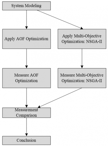
In the optimization of production machine flow shop scheduling, the makespan and total tardiness values will be compared before and after the implementation of NSGA-II multi-objective optimization. In general, the flowchart of the research design can be depicted in Figure 1.
Figure 1. Research design flowchart
2.1 Data collection
To test the system, the data tested was secondary data obtained from http://www.upv.es/gio/rruiz which consisted of 110 instances of data cases to be tested.
These data will then be used to model the system and processed using the multi-objective algorithm: NSGA-II.
A real-world case study in production scheduling: An automotive components factory in West Java faces production delays due to increasing customer order variation and machine limitations. Industry data: (1) Period: 6 months of historical data, (2) 15,200 job orders, (3) 12 machines with different capacities, (4) Fields: job_id, processing_time, due_date, machine_id, setup_time, priority, downtime_events.
The validation objectives are to minimize makespan (total completion time) and minimize total tardiness (lateness).
Validation methods: Algorithms compared: NSGA-II, AOF, MOEA/D, SPEA2. Evaluation metrics: Hypervolume, IGD, makespan, percentage of job lateness. Experiments: 30 replications for each algorithm.
2.2 System modeling
To obtain an optimal solution using the NSGA-II multi-objective algorithm, the flow shop production machine scheduling problem will be mathematically modeled in the form of a multi-objective equation consisting of several objective functions and constraints.
The multi-objective equation consists of two objective functions: one that defines the makespan value and one that defines the total tardiness.
Furthermore, it is necessary to define the desired solution variables, as NSGA-II optimization begins with random population initialization based on the definition of the solution variables.
2.3 NSGA-II stages
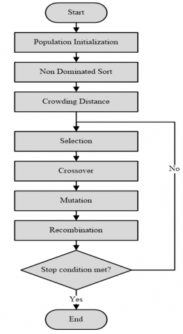
Multi-objective optimization: NSGA-II, which is used to find Pareto-optimal solutions from multi-objective mathematical models, can be divided into the following stages: 1) Population Initialization; 2) Non-Dominated Sort; 3) Crowding Distance; 4) Selection; 5) Genetic Operators: Crossover and Mutation; 6) Recombination.
In one of the several stages mentioned above, a more detailed procedure will be developed for applying NSGA-II to the problem of scheduling flow shop production machines. The general flow diagram of NSGA-II is shown in Figure 2.
Figure 2. NSGA-II flowchart
A review of existing methods in the literature shows that production scheduling approaches are still dominated by two main categories: mathematical optimization methods and machine learning-based methods. Mathematical optimization approaches, such as Mixed Integer Linear Programming (MILP), are inherently capable of producing exactly optimal solutions. However, the main limitation of MILP is its high computational complexity when the problem is enlarged to include more realistic numbers of machines, products, or constraints. This makes MILP difficult to implement in large-scale industrial scenarios that require fast and adaptive solutions.
In this context, multi-objective approaches based on evolutionary algorithms, such as NSGA-II, offer significant advantages. NSGA-II does not rely on complex mathematical models but instead utilizes the principles of population selection and evolution to find Pareto solutions that balance multiple objectives (e.g., minimizing makespan and tardiness simultaneously). Its primary advantage is its ability to explore a broad solution space at a relatively lower computational cost than exact methods, and it generates a set of Pareto solutions that can be readily used by decision-makers. Compared to RL, NSGA-II also does not require a long-term training process, making it more practical to apply to real industrial cases.
2.4 Measurement and comparison of optimization using NSGA-II
The results of multi-objective optimization of NSGA-II will be measured and compared with the results of optimization with AOF, by calculating and comparing the results of the two objective functions, namely makespan and total tardiness using AOF optimization with NSGA-II.
To evaluate the quality of the solution population generated by NSGA-II, the hypervolume indicator will be used. The hypervolume indicator is defined as the volume of all possible solutions dominated by the set of solutions generated by EMO. The larger the hypervolume value, the better the solution from EMO. The Monte Carlo approach [31] is used to estimate the hypervolume by calculating a set of random values in the solution space dominated by solutions from EMO.
Because NSGA-II is a stochastic algorithm, statistical analysis of the research results is necessary to compare them with a certain level of confidence. Normality and homogeneity tests will be performed first to determine the next test to compare the average results. The normality tests used are the Kolmogorov-Smirnov test and the Shapiro-Wilk test, while the homogeneity test uses the Levene test.
Research results that are normally distributed with homogeneous variance will be resolved using the ANOVA test, while for those that are normally distributed with non-homogeneous variance, the Welch test will be used. Specifically for research results that are not normally distributed, the Kruskal-Wallis test will be performed.
The Kruskal-Wallis test does not require the assumption of normality, but only requires that the data be ordinal or interval scaled and come from independent samples. This test procedure is based on the ranking of the data (ranking) rather than its actual values, so it is more robust to non-normal data distributions and the presence of outliers. Thus, Kruskal-Wallis provides a more flexible approach to comparing the medians of several groups when the ANOVA assumptions are not met. Case examples: (1) Comparing the makespan of 3 scheduling algorithms on several batch jobs, but the distribution of makespan is skewed, (2) Comparing the average waiting time per machine across 4 shift configurations, the data is not normal.
3.1 Mathematical model
The formulation of the makespan minimization problem with a mathematical model is carried out by Rego et al. [32] and Chen et al. [33] the following:
$\mathrm{M}(\mathrm{S})=\mathrm{C}_{\mathrm{m}, \mathrm{n}}$ (1)
$C_{m, n}=\max \left\{C_{m-1, n}, C_{m, n-1}\right\}+t_{m, n}$ (2)
where,
M(S) = makespan (time to process all jobs to completion)
Cm,n = completion time of job m on machine n
tm,n = processing time for job m on machine n
m = total number of jobs in the schedule
n = total number of machines in the schedule
In addition to formulating makespan, Huang et al. [34] formulated the problem of minimizing total tardiness with the following mathematical model:
$\mathrm{T}=\sum_{\mathrm{i}=0}^{\mathrm{n}} \max \left[0, \mathrm{C}_{\mathrm{i}}-\mathrm{d}_{\mathrm{i}}\right]$ (3)
where,
T = total tardiness (the total time a job can be completed earlier than its due date)
Ci = the complete time for all machines to complete a process on job i
Therefore, Eqs. (1)-(3) can be modeled as a multi-objective problem with the following mathematical model:
$\begin{aligned} & \operatorname{Min} \cdot \mathrm{Z}_{\mathrm{M}}=\max \left\{\mathrm{C}_{\mathrm{m}-1, \mathrm{n}}, \mathrm{C}_{\mathrm{m}, \mathrm{n}-1}\right\}+\mathrm{t}_{\mathrm{m}, \mathrm{n}} \\ & \operatorname{Min} \cdot \mathrm{Z}_{\mathrm{T}}=\sum_{i=0}^n \max \left[0, C_i-d_i\right]\end{aligned}$ (4)
where,
m = total number of jobs in the schedule
n = total number of machines in the schedule
tm,n = processing time for the mth job on the nth machine
$C_i$ = complete time for all machines to complete a process on job i (i = 1, ..., m)
3.2 Implementation of NSGA-II stages
The NSGA-II multi-objective optimization used to find a solution to the mathematical model of Equation 4 is divided into several stages as follows:
(1) Population Initialization
The population is initialized randomly, but must still comply with the constraints of the mathematical model.
(2) Non-Dominated Sort
The initialized population is then sorted based on non-dominance using the Fast Non-dominated Sorting algorithm defined by Deb as follows:
(a) For each individual p in population P, perform the following steps:
(i) Initialize Sp =$\varnothing$. This set will contain all individuals dominated by p.
(ii) Initialize np = 0. This indicates the number of individuals that dominate individual p.
(iii) For each individual q in P
·If p dominates q, add q to the set Sp. $\left(S_p=S_p \cup q\right)$
·If q dominates p, increment the dominance counter np. (np=np+1)
(iv) If np = 0, this means no individual dominates p, so p is in the first front; Assign p a rank of one (prank = 1). Add p to the first front $\left(F_1=F_1 \cup\{p\}\right)$
(b) Initialize the front counter with one (i = 1)
(c) As long as the i-th front is not empty (Ƒi ≠$\varnothing$), do the following:
(i) Q = $\varnothing$
(ii) For each individual p in front Ƒi
For each individual q in Sp
nq = nq - 1, decrement the dominance count for individual q
(iii) If nq = 0, then no individual in the next front dominates q, so qrank = i + 1. Add q to Q $(Q=Q \cup q)$.
(iv) Increment the front counter by one (i=i+1)
(v) Q becomes the next front (Ƒi = Q)
(3) Crowding Distance
Crowding distance is used as a comparison between two individuals in the same front, so that the resulting solution can represent the overall Pareto-optimal solution.
The method for calculating crowding distance is defined by Zheng et al. [35] and Zheng et al. [36] as follows:
(a) For each individual in front Ƒi, where n is the number of individuals
(b) Initialize the distance to zero for all individuals (Ƒi(dj)=0), where j represents the jth individual in front Ƒi
(c) For each objective function m
(i) Sort the individuals in front Ƒi i based on the objective value m
(ii) Assign infinite distances to the first and last individuals (I(d1)=$\infty$ and I(dn)=$\infty$)
(iii) For k ranging from 2 to (n-1)
$I\left(d_{\mathrm{k}}\right)=I\left(d_{\mathrm{k}}\right)+\frac{I(k+1) \cdot m-I(k-1) \cdot m}{\sum_m^{max }-\sum_m^{min } 1}$
I(k).m is the objective value m for individual k in I
(4) Selection
The roulette wheel selection method used is Roulette Wheel Selection. In the roulette wheel method, the parent chromosomes to be crossed over are selected based on their fitness values.
The fitness value of each chromosome is divided by the total fitness value of all chromosomes in the population. Each chromosome is considered a piece of the roulette wheel, with the size of the piece proportional to its fitness value. A target value between zero and one is randomly assigned. The roulette wheel is then spun N times, where N is the number of individuals or chromosomes in the population. In each spin, the chromosome with a fitness value below the target value is selected to become the parent for the next generation.
(5) Genetic Operators
The genetic operator used is Precedence Preservative Crossover (PPX) for crossover, and the mutation operators are removing and insert mutations. PPX can be explained as follows:
(a) A new string is randomly constructed from the alleles of the parent strings.
(b) A random number 1 or 2 is used to select the parent.
(c) f 1 is derived from the leftmost allele of the first parent, if 2 is derived from the leftmost allele of the second parent. The selected allele is then removed from both parents.
(d) The process continues until the characters in both parents are exhausted.
For example, two parents ABCDEF and CABFDE, and the random number 121122, will produce the new string ACBDFE.
In remove and insert mutations, one locus is randomly selected and the character at that position is deleted. A new locus is selected, and the previously deleted character is inserted.
(6) Recombination
The crossover and mutation population is then combined with the parent population, which is then selected using Non-Dominated Sort and Crowding Distance to obtain the next generation population.
3.3 Research results
The data used in this study is taken from Eva Instances: http://www.upv.es/gio/rruiz. The data consists of jobs ranging from 50 to 350 and machines ranging from 10 to 50.
Several samples will be taken from each job and machine. The data will then be tabulated using the format shown in Table 1.
Table 1. Production machine scheduling data table
|
Job/Machine |
M1 |
M2 |
M3 |
M4 |
.... |
Mn |
Due- Date |
|
J1 |
30 |
2 |
6 |
72 |
.... |
90 |
7 |
|
J2 |
20 |
30 |
80 |
70 |
.... |
80 |
8 |
|
.... |
.... |
.... |
.... |
.... |
.... |
.... |
.... |
|
Jn |
15 |
10 |
1 |
68 |
.... |
100 |
50 |
3.3.1 Optimizing production machine scheduling using AOF
The AOF method is a method for generating solutions that minimize makespan and total tardiness. In principle, this method applies single-objective optimization, such as the Genetic Algorithm, to multi-objective problems.
The two objective functions in Eq. (4) are combined into a new objective function using the addition operator (+), and each function is assigned a weight between 0 and 1, with the sum of the two weights necessarily equal to 1. The new objective function is the result of combining the two objective functions.
$C_\mathrm{m, n}=\max \left\{\mathrm{{C}_\mathrm{m-1, n}}, \mathrm{{C}_\mathrm{m, n-1}}\right\}+\mathrm{{t}_{m, n}}$ (5)
Eq. (4) is: $\operatorname{Min} Z=\alpha^*\left(\max \left\{\mathrm{C}_{\mathrm{i}-\mathrm{1}, \mathrm{j}}, \mathrm{C}_{\mathrm{i}, \mathrm{j}-1}\right\}+\mathrm{t}_{\mathrm{i}, \mathrm{j}}\right)+(1-\alpha) * \sum_{i=0}^n \max \left[0, C_i-d_i\right]$ where $\alpha$ is a weight with a value between 0 and 1 .
To optimize Eq. (4), a Genetic Algorithm is used, with the determination of the weight $\alpha$ carried out through research with variations of $\alpha$ = 0.1, 0.5 and 0.9, the data for which is tabulated in Tables 2 to 4.
Table 2. Production machine scheduling data table
|
Algorithm |
Hypervolume ↑ |
IGD ↓ |
Average Makespan (hours) ↓ |
% Job Terlambat ↓ |
|
NSGA-II |
0.72 ± 0.03 |
0.018 |
12.4 |
9.8% |
|
AOF |
0.68 ± 0.04 |
0.021 |
13.1 |
11.5% |
|
MOEA/D |
0.66 ± 0.05 |
0.024 |
13.3 |
12.1% |
|
SPEA2 |
0.64 ± 0.04 |
0.025 |
13.7 |
12.8% |
Table 3. AOF research results instance I_150_30
|
a |
Parameter |
Research Results |
||||
|
1 |
2 |
3 |
4 |
5 |
||
|
0,1 |
ZM |
11327 |
11153 |
11192 |
11200 |
11162 |
|
ZT |
133433 |
119589 |
123218 |
122785 |
129088 |
|
|
Number of Generations |
178 |
255 |
140 |
251 |
209 |
|
|
0,5 |
ZM |
11049 |
11332 |
11333 |
11184 |
11258 |
|
ZT |
130392 |
134616 |
138815 |
130638 |
130654 |
|
|
Number of Generations |
294 |
176 |
157 |
324 |
226 |
|
|
0,9 |
ZM |
11046 |
11345 |
11228 |
11464 |
10994 |
|
ZT |
121534 |
137081 |
139031 |
154819 |
129969 |
|
|
Number of Generations |
188 |
158 |
138 |
173 |
220 |
|
Table 4. AOF research results instance I_250_50
|
a |
Parameter |
Research Results |
||||
|
1 |
2 |
3 |
4 |
5 |
||
|
0,1 |
ZM |
19196 |
19731 |
19422 |
19689 |
19459 |
|
ZT |
453440 |
479169 |
522631 |
534560 |
482118 |
|
|
Number of Generations |
500 |
268 |
256 |
125 |
374 |
|
|
0,5 |
ZM |
19750 |
19459 |
19380 |
19584 |
19615 |
|
ZT |
508587 |
505159 |
471894 |
497512 |
539113 |
|
|
Number of Generations |
169 |
165 |
270 |
294 |
180 |
|
|
0,9 |
ZM |
19773 |
19599 |
19442 |
20015 |
19288 |
|
ZT |
503433 |
482715 |
499647 |
500287 |
468795 |
|
|
Number of Generations |
124 |
324 |
154 |
131 |
451 |
|
AOF weights can be dynamically adjusted. This approach leverages the distribution of solutions on the Pareto front, allowing the weights to reflect the trade-off balance between objectives that naturally emerges from the evolutionary algorithm. Furthermore, weights can be determined based on the decision maker's explicit preferences, for example through the integration of an interactive decision support system (DSS). This mechanism ensures that the selected solution is not only computationally optimal but also more closely aligned with practical needs and industry strategy. The dynamic weight approach also offers significant advantages. By adjusting weights based on the distribution of the Pareto front, the method is able to represent the trade-off between objectives in a more natural and adaptive manner.
To analyze the results of the AOF study above, normality and homogeneity tests were first conducted to determine the appropriate test for comparing the average results. The normality tests used were the Kolmogorov-Smirnov and Shapiro-Wilk tests, while the homogeneity test used Levene's test.
Research results with a normal distribution and homogeneous variances were compared using the ANOVA test, while those with a normal distribution and non-homogeneous variances were compared using the Welch test. For non-normally distributed results, the Kruskal-Wallis test was used. The statistical tests above were calculated using SPSS software, with the analysis results tabulated in the table below.
The results of the normality test in Table 5 with the Kolmogorov-Smirnov and Shapiro-Wilk tests show that the results of the AOF research for ZM, ZT and Generation at $\alpha$ = 0.1, 0.5 and 0.9 are normally distributed with a significance level of 0.05.
Table 5. Results of AOF normality test
|
Instance |
Alpha |
Kolmogorov-Smirnov |
Shapiro-Wilk |
|||||
|
Statistic |
df |
Sig. |
Statistic |
df |
Sig. |
|||
|
I_150_30 |
ZM |
0,10 |
0,339 |
5 |
0,062 |
0,794 |
5 |
0,073 |
|
0,50 |
0,201 |
5 |
0,200 |
0,889 |
5 |
0,353 |
||
|
0,90 |
0,204 |
5 |
0,200 |
0,945 |
5 |
0,702 |
||
|
ZT |
0,10 |
0,268 |
5 |
0,200 |
0,933 |
5 |
0,616 |
|
|
0,50 |
0,340 |
5 |
0,060 |
0,792 |
5 |
0,070 |
||
|
0,90 |
0,218 |
5 |
0,200 |
0,970 |
5 |
0,878 |
||
|
Number of Generations |
0,10 |
0,218 |
5 |
0,200 |
0,924 |
5 |
0,556 |
|
|
0,50 |
0,194 |
5 |
0,200 |
0,924 |
5 |
0,558 |
||
|
0,90 |
0,142 |
5 |
0,200 |
0,989 |
5 |
0,975 |
||
|
I_250_50 |
ZM |
0,10 |
0,208 |
5 |
0,200 |
0,932 |
5 |
0,611 |
|
0,50 |
0,173 |
5 |
0,200 |
0,977 |
5 |
0,920 |
||
|
0,90 |
0,139 |
5 |
0,200 |
0,986 |
5 |
0,962 |
||
|
ZT |
0,10 |
0,243 |
5 |
0,200 |
0,928 |
5 |
0,582 |
|
|
0,50 |
0,232 |
5 |
0,200 |
0,963 |
5 |
0,831 |
||
|
0,90 |
0,321 |
5 |
0,102 |
0,847 |
5 |
0,186 |
||
|
Number of Generations |
0,10 |
0,203 |
5 |
0,200 |
0,977 |
5 |
0,917 |
|
|
0,50 |
0,319 |
5 |
0,107 |
0,803 |
5 |
0,085 |
||
|
0,90 |
0,316 |
5 |
0,115 |
0,827 |
5 |
0,131 |
||
|
I_350_30 |
ZM |
0,10 |
0,244 |
5 |
0,200 |
0,956 |
5 |
0,780 |
|
0,50 |
0,176 |
5 |
0,200 |
0,972 |
5 |
0,886 |
||
|
0,90 |
0,203 |
5 |
0,200 |
0,890 |
5 |
0,356 |
||
|
ZT |
0,10 |
0,315 |
5 |
0,118 |
0,777 |
5 |
0,052 |
|
|
0,50 |
0,300 |
5 |
0,159 |
0,893 |
5 |
0,374 |
||
|
0,90 |
0,215 |
5 |
0,200 |
0,969 |
5 |
0,868 |
||
|
Number of Generations |
0,10 |
0,268 |
5 |
0,200 |
0,919 |
5 |
0,525 |
|
|
0,50 |
0,307 |
5 |
0,139 |
0,840 |
5 |
0,166 |
||
|
0,90 |
0,260 |
5 |
0,200 |
0,919 |
5 |
0,524 |
||
The results of the homogeneity test in Table 5 using Levene's test indicate that the AOF research results for ZM, ZT, and Generation at α = 0.1, 0.5, and 0.9 have homogeneous variances with a significance level of 0.05 (the Sig. column in Table 6 is greater than 0.05).
Table 6. AOF research results instance I_350_50
|
a |
Parameter |
Research Results |
||||
|
1 |
2 |
3 |
4 |
5 |
||
|
0,1 |
ZM |
25243 |
25284 |
25435 |
25451 |
25518 |
|
ZT |
2193090 |
2274710 |
2232403 |
2329579 |
2286649 |
|
|
Number of Generations |
263 |
300 |
262 |
219 |
378 |
|
|
0,5 |
ZM |
25432 |
25596 |
25407 |
25537 |
25415 |
|
ZT |
2311256 |
2254846 |
2260478 |
2355096 |
2236693 |
|
|
Number of Generations |
289 |
282 |
237 |
103 |
244 |
|
|
0,9 |
ZM |
25288 |
25654 |
25179 |
25422 |
25193 |
|
ZT |
2241915 |
2208694 |
2150877 |
2309797 |
2262883 |
|
|
Number of Generations |
237 |
161 |
318 |
114 |
195 |
|
Based on the results of the two tests above, the AOF experimental results are normally distributed with homogeneous variances. Therefore, the ANOVA test was used to compare the average values of ZM, ZT, and Generation at α = 0.1, 0.5, and 0.9 with the test results tabulated in the Table 7.
Table 7. Results of AOF homogeneity test
|
Instance |
Levene Statistic |
df1 |
df2 |
Sig. |
|
|
I_150_30 |
ZM |
3,126 |
2 |
12 |
0,081 |
|
ZT |
1,865 |
2 |
12 |
0,197 |
|
|
Number of Generations |
2,694 |
2 |
12 |
0,108 |
|
|
I_250_50 |
ZM |
1,084 |
2 |
12 |
0,369 |
|
ZT |
1,948 |
2 |
12 |
0,185 |
|
|
Number of Generations |
2,130 |
2 |
12 |
0,162 |
|
|
I_350_30 |
ZM |
0,225 |
2 |
12 |
0,801 |
|
ZT |
0,790 |
2 |
12 |
0,476 |
|
|
Number of Generations |
20,484 |
2 |
12 |
0,125 |
|
The ANOVA test results show that the average values of ZM, ZT, and Generations do not differ significantly for α=0.1, 0.5, and 0.9 at a significance level of 0.05 (the Sig. column in Table 7 is greater than 0.05). This means that changes in α do not significantly affect changes in the average values of the first objective function (ZM), the second objective function (ZT), or the number of generations. The Genetic Algorithm for AOF optimization applies the same PPX and Remove and Insert operators as the Genetic Operators for the NSGA-II stage with parameters tabulated in Table 8.
Table 8. Results of ANOVA AOF test
|
Instance |
Sum of Squares |
df |
Mean Square |
F |
Sig. |
||
|
I_150_30 |
ZM |
Between Groups |
1531,600 |
2 |
765,800 |
0,039 |
0,961 |
|
Within Groups |
232752,800 |
12 |
19396,067 |
|
|
||
|
Total |
234284,400 |
14 |
|
|
|
||
|
ZT |
Between Groups |
307991120,400 |
2 |
153995560,200 |
2,350 |
0,138 |
|
|
Within Groups |
786520738,000 |
12 |
65543394,833 |
|
|
||
|
Total |
1094511858,400 |
14 |
|
|
|
||
|
Number of Generations |
Between Groups |
9004,800 |
2 |
4502,400 |
1,567 |
0,248 |
|
|
Within Groups |
34475,600 |
12 |
2872,967 |
|
|
||
|
Total |
43480,400 |
14 |
|
|
|
||
|
I_250_50 |
ZM |
Between Groups |
38488,133 |
2 |
19244,067 |
0,389 |
0,686 |
|
Within Groups |
593259,600 |
12 |
49438,300 |
|
|
||
|
Total |
631747,733 |
14 |
|
|
|
||
|
ZT |
Between Groups |
491090575,600 |
2 |
245545287,800 |
0,384 |
0,689 |
|
|
Within Groups |
7674834746,400 |
12 |
639569562,200 |
|
|
||
|
Total |
8165925322,000 |
14 |
|
|
|
||
|
Number of Generations |
Between Groups |
21612,133 |
2 |
10806,067 |
0,727 |
0,503 |
|
|
Within Groups |
178319,200 |
12 |
14859,933 |
|
|
||
|
Total |
199931,333 |
14 |
|
|
|
||
|
I_350_30 |
ZM |
Between Groups |
29147,733 |
2 |
14573,867 |
0,414 |
0,670 |
|
Within Groups |
422279,600 |
12 |
35189,967 |
|
|
||
|
Total |
451427,333 |
14 |
|
|
|
||
|
ZT |
Between Groups |
407911697,200 |
2 |
203955848,600 |
0,125 |
0,884 |
|
|
Within Groups |
19575430524,400 |
12 |
1631285877,033 |
|
|
||
|
Total |
19983342221,600 |
14 |
|
|
|
||
|
Number of Generations |
Between Groups |
8880,933 |
2 |
4440,467 |
0,257 |
0,777 |
|
|
Within Groups |
207110,000 |
12 |
17259,167 |
|
|
||
|
Total |
215990,933 |
14 |
|
|
|
||
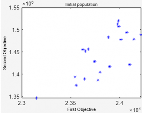
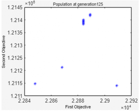
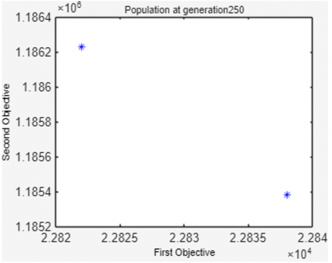
To show the population changes related to the increase in generations, Figure 3 displays the Genetic Algorithm population for production machine scheduling at the time of population initialization, the 50th, 125th, 250th and 294th generations. It turns out that the value of the 1st objective function (ZM) and the value of the 2nd objective function (ZT) are always better than the previous generation.
To strengthen the validity of the results, clarification of the parameter tuning method is needed. One commonly used approach is grid search, where parameter combinations are systematically tested to identify the best configuration based on performance indicators (e.g., hypervolume or spread). By trying several parameter combinations (e.g., PopSize = {50, 100, 200}, Crossover = {0.8, 0.9, 1.0}, Mutation = {0.05, 0.1, 0.2}. These parameter combinations are presented in Table 9.
Table 9. Grid search parameter NSGA-II
|
Population Size |
Crossover Rate |
Mutation Rate |
IGD (↓) |
HV (↑) |
Time (s) |
|
50 |
0.8 |
0.05 |
0.032 |
0.68 |
25 |
|
100 |
0.9 |
0.10 |
0.027 |
0.72 |
48 |
|
200 |
0.9 |
0.20 |
0.024 |
0.74 |
95 |
Another, more adaptive alternative is automatic parameter tuning, such as adaptive parameter control or self-adaptive evolutionary strategies, which dynamically adjust parameter values during the evolution process. Implementing these tuning methods makes experimental results more credible, replicable, and relevant for real-world applications in industrial environments.
3.3.2 Optimizing production machine scheduling using NSGA-II
To efficiently obtain the best set of Pareto-optimal solutions, experiments are needed to determine the smallest number of generations required to obtain them.
Applying Pareto solutions in the context of production scheduling presents its own challenges, as optimization results generated by multi-objective algorithms are often only displayed in tables or static graphs.
Therefore, integrating Pareto solutions into a Decision Support System (DSS) or interactive tool is a strategic step to ensure that the resulting solutions are not only theoretical but also operational. Future research will attempt to utilize an Integrated DSS.
Through a DSS, Pareto solutions, which represent trade-offs between objectives (e.g., minimizing makespan, total delay, and increasing machine utilization), can be visualized in interactive graphs such as scatter plots or parallel coordinate plots. With this display, decision-makers can understand the distribution patterns of solutions and select the alternative that best aligns with company priorities.
The quality of the Pareto-optimal solution sets from different generations is compared based on the average estimate of the hypervolume indicator.
The hypervolume indicator is estimated using a Monte Carlo approach [37-39], which normalizes all objective function values between 0 and 1, then generates a random set of objective function values and tests each random objective function value to see whether it is dominated by one of the Pareto-optimal solutions.
The research for hypervolume estimation was conducted three times for each instance in the same generation, the results of which are tabulated in Table 10.
Table 10. Genetic algorithm parameters for AOF
|
No. |
Parameter Name |
Value |
|
1 |
Population Size |
20 |
|
2 |
Weight (a) |
0,1 |
|
3 |
Probability of Crossover (Pc) |
0,9 |
|
4 |
Probability of Mutation (Pm) |
0,1 |
Table 11. Results of NSGA-II hypervolume estimation research
|
Instance |
Hypervolume Estimation in Research |
Average |
||||
|
1 |
2 |
3 |
4 |
5 |
||
|
I_350_30 |
0,62454 |
0,53367 |
0,86426 |
0,76701 |
0,76477 |
0,7108500 |
|
I_250_50 |
0,74693 |
0,56053 |
0,62099 |
0,43587 |
0,79323 |
0,6315100 |
|
I_150_30 |
0,44204 |
0,54995 |
0,69228 |
0,7856 |
0,62527 |
0,6190280 |
The normality test using SPSS on the data in Table 11 is tabulated in Table 12. The normality test assesses the normality of data distribution. This test is the most commonly used for parametric statistical analysis. Normally distributed data is a prerequisite for parametric tests. For data that does not have a normal distribution, non-parametric tests are used for analysis.
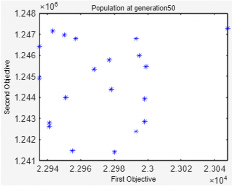
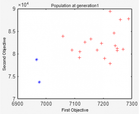
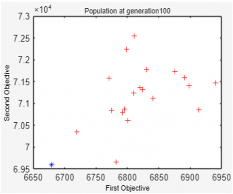
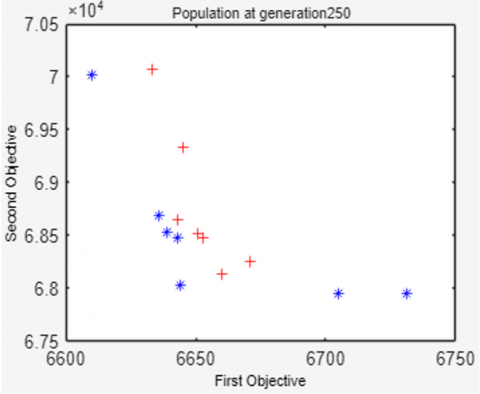
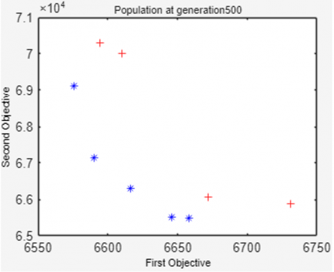
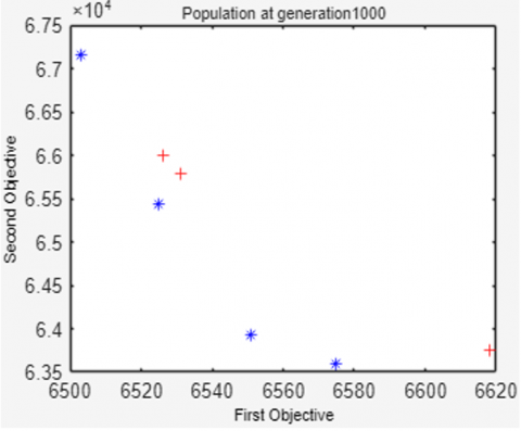
To show population changes related to increasing generations, Figure 4 displays the NSGA-II population at the time of population initialization, the 100th, 250th, 500th, 750th and 1000th generations.
Figure 4 shows that the 20 solutions in the population are increasingly evenly distributed, approaching the Pareto-optimal solution as the number of generations increases. As generations increase, the values of the first and second objective functions decrease simultaneously. It can be seen that of the 20 resulting solutions, not all are Pareto-optimal. In this example, only 12 Pareto-optimal solutions are on front 1 (symbolized by a blue '*'), while the other 8 solutions are on front 2 (symbolized by a red '+').
The population obtained in the 1000th generation of NSGA-II is tabulated in Table 12.
Table 12. Normality test results of NSGA-II hypervolume estimation
|
Instances |
Kolmogorov-Smirnov |
Shapiro-Wilk |
|||||
|
Statistic |
df |
Sig. |
Statistic |
df |
Sig. |
||
|
Hypervolume |
I_150_30 |
0,119 |
5 |
0,200 |
0,997 |
5 |
0,997 |
|
I_250_50 |
0,189 |
5 |
0,200 |
0,963 |
5 |
0,827 |
|
|
I_350_30 |
0,260 |
5 |
0,200 |
0,944 |
5 |
0,691 |
|
|
I_350_50 |
0,315 |
5 |
0,117 |
0,809 |
5 |
0,096 |
|
|
I_50_50 |
0,237 |
5 |
0,200 |
0,910 |
5 |
0,470 |
|
Table 13 is a table of NSGA II parameters, which consists of: Population size = 20. Advantages, fast computation per generation. Generations = 1000. Many generations good for allowing convergence. Pc = 0.9 common and reasonable value. Emphasizes the exploitation of gene combinations. Pm = 0.1 somewhat high for some representations (mutation is typically 0.001–0.1 depending on the representation).
Table 13. NSGA-II parameters
|
No. |
Parameter Name |
Value |
|
1 |
Population Number |
20 |
|
2 |
Generation |
1000 |
|
3 |
Probability of Crossover (Pc) |
0,9 |
|
4 |
Probability of Mutation (Pm) |
0,1 |
Table 14. NSGA-II population at the 1000th generation
|
Solution to- |
ZM |
ZT |
Front |
Crowding Distance |
|
1 |
25101 |
2305256 |
1 |
0,321962797 |
|
2 |
25075 |
2313357 |
1 |
0,281232594 |
|
3 |
25078 |
2308285 |
1 |
0,067711391 |
|
4 |
25076 |
2312753 |
1 |
0,263258517 |
|
5 |
25058 |
2315153 |
1 |
0,900309604 |
|
6 |
25078 |
2308285 |
1 |
0 |
|
7 |
25077 |
2308887 |
1 |
0,263148123 |
|
8 |
25079 |
2307208 |
1 |
0,357273681 |
|
9 |
25137 |
2302717 |
1 |
65535 |
|
10 |
25078 |
2308285 |
1 |
0,041492922 |
|
11 |
25016 |
2320834 |
1 |
65535 |
|
12 |
25101 |
2305256 |
1 |
0,405264769 |
|
13 |
25021 |
2334534 |
2 |
65535 |
|
14 |
25158 |
2304022 |
2 |
65535 |
|
15 |
25087 |
2308031 |
2 |
0,726049629 |
|
16 |
25077 |
2308971 |
2 |
0,613319063 |
|
17 |
25078 |
2308358 |
2 |
0,018016365 |
|
18 |
25078 |
2308358 |
2 |
0 |
|
19 |
25059 |
2322840 |
2 |
1,246560645 |
|
20 |
25078 |
2308358 |
2 |
0 |
Table 14 is the result of the NSGA-II population at the 1000th generation.
3.4 Comparison of AOF and NSGA-II
Solutions to multi-objective problems can be compared using dominance.
The i-th solution is declared better than the j-th solution if it dominates the j-th solution. The i-th solution dominates the j-th solution if all the objective function values of the i-th solution are no worse than the j-th solution, and at least one objective function value of the i-th solution is better than the objective function of the j-th solution.
Table 15 shows that a dominance comparison is performed between the AOF Genetic Algorithm solution for α = 0.1 and the NSGA-II solution. The symbol 'M' is used to indicate dominance, 'D' =100 to indicate dominance, and '-' to indicate non-dominance of the solutions.
Table 15. Comparison of the dominance of the AOF solution with the NSGA-II solution for instance I_150_30
|
Solution |
NSGA-II |
|||||||||
|
1 |
2 |
3 |
4 |
5 |
6 |
7 |
8 |
9 |
10 |
|
|
AOF1 |
- |
- |
- |
- |
- |
- |
- |
- |
- |
- |
|
AOF2 |
- |
- |
- |
- |
- |
- |
- |
- |
- |
- |
|
AOF3 |
- |
- |
- |
- |
- |
- |
- |
- |
- |
- |
|
AOF4 |
- |
- |
- |
- |
- |
- |
- |
- |
- |
- |
|
AOF5 |
- |
- |
- |
- |
- |
- |
- |
- |
- |
- |
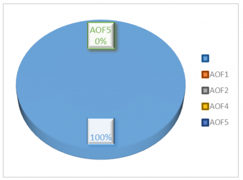
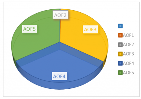
Figure 5 is a 2-dimensional image of the shape of comparison of the dominance of the AOF solution with the NSGA-II solution for instance I_150_30.
Figure 5. Comparison of the dominance of the AOF solution with the NSGA-II solution for instance I_150_30
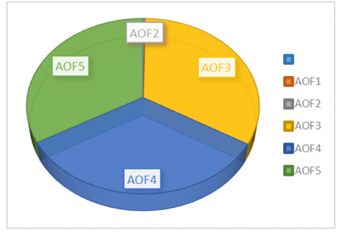
Figure 6 is a 2-dimensional image of the shape of comparison of the dominance of the AOF solution with the NSGA-II solution for instance I_250_50.
Figure 6. Comparison of the dominance of the AOF solution with the NSGA-II solution for instance I_250_50
Figure 7 is a 2-dimensional image of the shape of comparison of the dominance of the AOF solution with the NSGA-II solution for instance I_350_30.
Figure 7. Comparison of the dominance of the AOF solution with the NSGA-II solution for instance I_350_30
The comparison of the dominance of AOF solutions with NSGA-II solutions in Tables 16 and 17 shows that there are always AOF solutions dominated by NSGA-II solutions, while no AOF solutions dominate NSGA-II solutions. This indicates that the Pareto-optimal NSGA-II solution successfully provides a better solution than the AOF solution.
Table 16. Comparison of the dominance of the AOF solution with the NSGA-II solution for instance I_250_50
|
Solution |
NSGA-II |
|||||||||
|
1 |
2 |
3 |
4 |
5 |
6 |
7 |
8 |
9 |
10 |
|
|
AOF1 |
- |
- |
- |
- |
- |
- |
- |
- |
- |
- |
|
AOF2 |
- |
- |
D |
- |
D |
- |
- |
- |
D |
D |
|
AOF3 |
D |
D |
D |
D |
D |
D |
D |
D |
D |
D |
|
AOF4 |
D |
D |
D |
D |
D |
D |
D |
D |
D |
D |
|
AOF5 |
D |
D |
D |
D |
D |
D |
D |
D |
D |
D |
Table 17. Comparison of the dominance of the AOF solution with the NSGA-II solution for instance I_350_30
|
Solution |
NSGA-II |
|||||||||
|
1 |
2 |
3 |
4 |
5 |
6 |
7 |
8 |
9 |
10 |
|
|
AOF1 |
D |
D |
D |
D |
D |
D |
D |
D |
D |
D |
|
AOF2 |
- |
- |
- |
- |
- |
- |
- |
- |
- |
- |
|
AOF3 |
D |
D |
D |
- |
D |
D |
D |
D |
- |
- |
|
AOF4 |
D |
D |
D |
D |
D |
D |
D |
D |
D |
D |
|
AOF5 |
D |
D |
D |
D |
D |
D |
D |
D |
D |
D |
Based on the comparison above, it is clear that the population of Pareto-optimal NSGA-II solutions is superior, successfully dominating 100% of the AOF system solutions. Similarly, the comparison of NSGA-II solutions with AOF solutions shows that the population of Pareto-optimal NSGA-II solutions is superior, successfully dominating 100% of the AOF solutions.
The population of Pareto-optimal solutions can be used to provide managers with several alternative solutions. Pareto-optimal solutions are optimal multi-objective optimization solutions with trade-offs across all objectives, so all Pareto-optimal solutions are equally good. Therefore, managers still need to make informed decisions about which solution to implement in the company.
From the results of the research and discussion that has been done, it can be concluded that in NSGA-II, 20 solutions in the population are increasingly evenly distributed approaching the Pareto-optimal solution with increasing number of generations, and along with increasing generations, the makespan and total tardiness values will be increasingly minimal together. The application of NSGA-II operators, namely Nondominated Sorted, Crowding Distance, PPX (Precedence Preservative Crossover) and remove and insert mutations successfully obtained a solution to the mathematical model of production machine scheduling. The results of the analysis of the Pareto-optimal solution produced by NSGA-II show that the Pareto-optimal solution is better by dominating 100% of the solution from the system produced by the Genetic Algorithm with Aggregate of Function (AOF).
The author expresses his deepest gratitude to the Ministry of Higher Education, Science, and Technology of the Republic of Indonesia (KEMDIKTISAINTEK) for the support provided in the form of a national competitive grant with contract number: 122/C3/DT.05.00/PL/2025.
[1] Ɖurasević, M., Jakobović, D. (2023). Heuristic and metaheuristic methods for the parallel unrelated machines scheduling problem: A survey. Artificial Intelligence Review, 56(4): 3181-3289. https://doi.org/10.1007/s10462-022-10247-9
[2] Yan, Q., Wu, W., Wang, H. (2022). Deep reinforcement learning for distributed flow shop scheduling with flexible maintenance. Machines, 10(3): 210. https://doi.org/10.3390/machines10030210
[3] Aich, W., Basem, A., Sawaran Singh, N.S., Mausam, K., et al. (2025). Two-layer energy scheduling of electrical and thermal smart grids with energy hubs including renewable and storage units considering energy markets. Scientific Reports, 15(1): 25079. https://doi.org/10.1038/s41598-025-09960-6
[4] Jansen, K., Klein, K.M., Maack, M., Rau, M. (2022). Empowering the configuration-IP: New PTAS results for scheduling with setup times. Mathematical Programming, 195(1): 367-401. https://doi.org/10.1007/s10107-021-01694-3
[5] Sonata, F. (2015). Sistem penjadwalan mesin produksi menggunakan algoritma johnson dan campbell. Jurnal Buana Informatika 6(3): 173-182. https://doi.org/10.24002/jbi.v6i3.430
[6] Liang, Z., Zhong, P., Liu, M., Zhang, C., Zhang, Z. (2022). A computational efficient optimization of flow shop scheduling problems. Scientific Reports, 12(1): 845. https://doi.org/10.1038/s41598-022-04887-8
[7] Rana, N., Abd Latiff, M.S., Abdulhamid, S.I.M., Misra, S. (2022). A hybrid whale optimization algorithm with differential evolution optimization for multi-objective virtual machine scheduling in cloud computing. Engineering Optimization, 54(12): 1999-2016. https://doi.org/10.1080/0305215X.2021.1969560
[8] Ghosh, A., Deb. K., Goodman, E, Averill, R. (2023). An interactive knowledge-based multiobjective evolutionary algorithm framework for practical optimization problems. IEEE Transactions on Evolutionary Computation, 28(1): 223-237. https://doi.org/10.1109/TEVC.2023.3259339
[9] Ying, K.C., Pourhejazy, P., Huang, T.C. (2024). Exploring the development trajectory of single-machine production scheduling. Annals of Operations Research, 1-26. https://doi.org/10.1007/s10479-024-06395-6
[10] Xu, W, Wang, X., Guo, Q., Song, X., et al. (2023). Evolutionary process for engineering optimization in manufacturing applications: Fine brushworks of single-objective to multi-objective/many-objective optimization. Processes, 11(3): 693. https://doi.org/10.3390/pr11030693
[11] Karacan, I., Senvar, O., Bulkan, S. (2023). A novel parallel simulated annealing methodology to solve the no-wait flow shop scheduling problem with earliness and tardiness objectives. Processes, 11(2): 454. https://doi.org/10.3390/pr11020454
[12] Kurt, A. (2025). Integrating sequence-dependent setup times and blocking in hybrid flow shop scheduling to minimize total tardiness. International Journal of Industrial Engineering Computations, 16(1): 147-158. https://doi.org/10.5267/j.ijiec.2024.10.005
[13] Nejjarou, O., Aqil, S., Lahby, M. (2024). Hybrid meta-heuristic solving no-wait flow shop scheduling minimizing maximum tardiness. Evolutionary Intelligence, 17(5): 3935-3959. https://doi.org/10.1007/s12065-024-00965-0
[14] Ezugwu, A.E.S. (2024). Metaheuristic optimization for sustainable unrelated parallel machine scheduling: A concise overview with a proof-of-concept study. IEEE Access, 12: 3386-3416. https://doi.org/10.1109/ACCESS.2023.3347047
[15] Hajji, M.K., Hadda, H., Dridi, N. (2023). Makespan minimization for the two-stage hybrid flow shop problem with dedicated machines: A comprehensive study of exact and heuristic approaches. Computation, 11(7): 137. https://doi.org/10.3390/computation11070137
[16] Yusriski, R., Nasution, A.R.K., Lukas, Wijayanti, L., Octaviani, S. (2023). A two-machine flow shop batch scheduling model to minimize total actual flow time. Jurnal Teknik Industri, 25(2): 179-194. https://doi.org/10.9744/jti.25.2.179-194
[17] Jerbi, B., Kanoun, S., Kamoun, H. (2025). Multi-objective mathematical programs to minimize the makespan, the patients’ flow time, and doctors’ workloads variation using dispatching rules and genetic algorithm. Yugoslav Journal of Operations Research, 35(2): 365-382. https://doi.org/10.2298/YJOR240115032J
[18] Wang, H., Li, R., Gong, W. (2023). Minimizing tardiness and makespan for distributed heterogeneous unrelated parallel machine scheduling by knowledge and pareto-based memetic algorithm. Egyptian Informatics Journal, 24(3): 100383. https://doi.org/10.1016/j.eij.2023.05.008
[19] Mousavi, S.M., Shahnazari-Shahrezaei, P. (2023). Minimizing the makespan and total tardiness in hybrid flow shop scheduling with sequence-dependent setup times. Management and Production Engineering Review, 14(1): 13-24. https://doi.org/10.24425/mper.2023.145362
[20] Wahyudi, C., Sirait, S., Rahmadani, E., Sapta, A., Saragih, S.R.D. (2021). Efektivitas pembelajaran daring melalui whatsapp group terhadap kemampuan pemahaman konsep matematis siswa. Jurnal Pena Edulasi, 8(1): 1-6. https://doi.org/10.54314/jpe.v8i1.491
[21] Anam, R.A.S., Sapta, A., Handayani, M., Masbukhin, F. A.A., et al. (2024). Optimalisasi penggunaan aplikasi digital dalam proses pembelajaran di sekolah dasar pada kota serang. Jurnal Pemberdayaan Sosial dan Teknologi Masyarakat, 4(2): 164-169. https://doi.org/10.54314/jpstm.v4i2.2253
[22] Hutagalung, J., Azlan, A. (2020). Pemanfaatan gis dan ahp dalam penerimaan dana bos jenjang SMA. JURTEKSI (Jurnal Teknologi Dan Sistem Informasi), 6(3): 221-230.
[23] Labidi, H., Azzouna, N.B., Hassine, K., Gouider, M.S. (2023). An improved genetic algorithm for solving the multi-objective vehicle routing problem with environmental considerations. Procedia Computer Science, 225: 3866-3875. https://doi.org/10.1016/j.procs.2023.10.382
[24] Ransikarbum, K., Wattanasaeng, N., Madathil, S.C. (2023). Analysis of multi-objective vehicle routing problem with flexible time windows: The implication for open innovation dynamics. Journal of Open Innovation: Technology, Market, and Complexity, 9(1): 100024. https://doi.org/10.1016/j.joitmc.2023.100024
[25] Nielsen, M.K., Jacobsen, A.M., Carstensen, J.L., Nielsen, M.T., Tambo, T. (2024). Industrial R&D project portfolio selection method using a multi-objective optimization program: A conceptual quantitative framework. Journal of Industrial Engineering and Management, 17(1): 217-234. https://doi.org/10.3926/jiem.6552
[26] Araújo, G.R., Gomes R, Ferrão. P, Gomes, M.G. (2024). Optimizing building retrofit through data analytics: A study of multi-objective optimization and surrogate models derived from energy performance certificates: Optimizing building retrofit through data analytics. Energy and Built Environment, 5(6): 889-899. https://doi.org/10.1016/j.enbenv.2023.07.002
[27] Preuß, O.L., Rook, J., Trautmann, H. (2024). On the potential of multi-objective automated algorithm configuration on multi-modal multi-objective optimisation problems. In Applications of Evolutionary Computation: 27th European Conference (EvoApplications 2024), Aberystwyth, UK, pp. 305-321. https://doi.org/10.1007/978-3-031-56852-7_20
[28] Deb, K., Tiwari, S. (2008). Omni-optimizer: A generic evolutionary algorithm for single and multi-objective optimization. European Journal of Operational Research, 185(3): 1062-1087. https://doi.org/10.1016/j.ejor.2006.06.042
[29] Rahimi-Vahed, A.R., Mirghorbani, S.M. (2007). A multi-objective particle swarm for a flow shop scheduling problem. Journal of Combinatorial Optimization, 13(1): 79-102. https://doi.org/10.1007/s10878-006-9015-7
[30] Vukadinović, A., Radosavljević, J., Đorđević, A., Protić, M., Petrović, N. (2021). Multi-objective optimization of energy performance for a detached residential building with a sunspace using the NSGA-II genetic algorithm. Solar Energy, 224: 1426-1444. https://doi.org/10.1016/j.solener.2021.06.082
[31] Nemeth, C., Fearnhead, P. (2021). Stochastic gradient Markov chain monte Carlo. Journal of the American Statistical Association, 116(533): 433-450. https://doi.org/10.1080/01621459.2020.1847120
[32] Rego, M.F., Pinto, J.C.E., Cota, L.P., Souza, M.J. (2022). A mathematical formulation and an NSGA-II algorithm for minimizing the makespan and energy cost under time-of-use electricity price in an unrelated parallel machine scheduling. PeerJ Computer Science, 8: e844. https://doi.org/10.7717/peerj-cs.844
[33] Chen, Y., Tsai, Y.C., Chou, F.D. (2023). An evaluation of mathematical programming and lower-bound methods for hybrid flow shop problems with a makespan criterion. IEEE Access, 11: 41368-41386. https://doi.org/10.1109/ACCESS.2023.3268214
[34] Huang, K.W., Lin, B.M. (2025). Deep q-networks for minimizing total tardiness on a single machine. Mathematics, 13(1): 62. https://doi.org/10.3390/math13010062
[35] Zheng, W., Doerr, B. (2024). Approximation guarantees for the non-dominated sorting genetic algorithm II (NSGA-II). IEEE Transactions on Evolutionary Computation, 29(4): 891-905. https://doi.org/10.1109/TEVC.2024.3402996
[36] Zheng, W., Gao, Y., Doerr, B. (2024). A crowding distance that provably solves the difficulties of the NSGA-II in many-objective optimization. Neural and Evolutionary Computing. arXiv preprint arXiv: 2407.17687. https://doi.org/10.48550/arXiv.2407.17687
[37] Abubakar, A., Borkor, R.N., Amoako-Yirenkyi, P. (2023). Stochastic optimal selection and analysis of allowable photovoltaic penetration level for grid-connected systems using a hybrid NSGAII-MOPSO and monte Carlo method. International Journal of Photoenergy, 2023(1): 5015315. https://doi.org/10.1155/2023/5015315
[38] Liu, Y., Zhu, Y., Wang, J., Hu, R., et al. (2025). A multi-objective molecular generation method based on pareto algorithm and monte Carlo tree search. Advanced Science, 12(20): 2410640. https://doi.org/10.1002/advs.202410640
[39] Yen, L.W., Thinakaran, R., Somasekar, J. (2025). Machine learning-based denoising techniques for monte Carlo rendering: A literature review. Machine Learning, 16(2). https://doi.org/10.14569/IJACSA.2025.0160259