Huu Chien Pham![]() | Xuan Cuong Ngo
| Xuan Cuong Ngo![]() | Nhu Y. Do*
| Nhu Y. Do*![]()
© 2025 The authors. This article is published by IIETA and is licensed under the CC BY 4.0 license (http://creativecommons.org/licenses/by/4.0/).
OPEN ACCESS
The effective utilization of wind energy strongly relies on accurate power forecasting, in which short-term prediction plays a crucial role in grid operation. In practice, measurement data are often incomplete due to data loss. Existing studies typically address this issue by either focusing on data imputation, developing forecasting models based on deep learning or machine learning (DL/ML), or integrating numerical weather prediction (NWP) models and data security. However, only a limited number of approaches effectively combine robust imputation with powerful time-series forecasting models, while also ensuring comprehensive evaluation under various data loss scenarios and maintaining both interpretability and practical applicability. Moreover, regional characteristics significantly influence forecasting methods and wind power management strategies. To address these challenges, this paper proposes a hybrid XGBoost-GRU model for short-term wind power forecasting, with a case study in Southern Vietnam. Experimental results demonstrate that the proposed model outperforms the baseline GRU model by achieving higher predictive accuracy and maintaining stable performance under different data conditions.
wind power forecasting, artificial intelligence, XGBoost–GRU, GRU, XGBoost
In the context of the global energy transition aimed at reducing greenhouse gas emissions and mitigating climate change, renewable energy sources, particularly wind power, are playing an increasingly critical role [1, 2]. The effective utilization of wind energy largely depends on the accuracy of power forecasting, with short-term prediction being essential for grid regulation, operational optimization, and minimizing contingency costs [1]. Nevertheless, the rapidly changing, nonlinear, and unstable characteristics of wind make accurate forecasting a challenging task [3].
In practical operations, measurement data obtained from wind turbine SCADA systems or numerical weather prediction (NWP) models are often incomplete due to data loss [4, 5]. The causes may include sensor malfunctions, transmission line disturbances, equipment maintenance, or recording errors. Such data loss considerably degrades the quality of training and input datasets, thereby reducing forecasting accuracy. The challenge becomes even more critical when the loss rate is high or occurs over continuous periods [6].
A common approach to address this issue is to recover missing data prior to forecasting, treating data reconstruction as an independent preprocessing step. In the study [7], the time-series characteristics of wind power data were analyzed, and the impact of different data loss scenarios on forecasting errors was evaluated, leading to the development of a compensation method based on interpolation and multivariate correlation analysis. Similarly, in the document [8] employed a combination of Gaussian Process Regression and Multiple Imputation to restore wind power data, achieving significantly higher forecasting accuracy compared to traditional interpolation methods. The main advantage of this approach is that it enables the direct use of existing forecasting models once the input data have been completed. However, its limitation lies in the strong dependence of forecasting accuracy on the quality of the imputation process, with a potential risk of error propagation if the reconstructed data fail to accurately reflect reality.
Instead of separating the recovery and prediction stages, some studies have developed hybrid models that simultaneously integrate forecasting and missing data handling during the training process. According to research [9], a hybrid approach combining Empirical Mode Decomposition (EMD) and Long Short-Term Memory (LSTM) was proposed, where LSTM is trained on signal-processed data reconstructed from component analysis, thereby mitigating the impact of random data loss. The Wasserstein GAN with Gradient Penalty was employed to generate high-quality synthetic data, which were then incorporated into the training set to enhance forecasting performance under missing input conditions [10]. The main advantage of such hybrid approaches is the reduction of cumulative errors while leveraging the feature learning capability of deep models. However, these methods generally involve more complex training procedures and require higher computational resources.
Some studies have focused on enhancing the robustness of forecasting models against data loss by improving network architectures or optimizing input feature selection. In the document [11] proposed a short-term wind power forecasting method based on multivariate signal decomposition combined with input variable selection, enabling the model to rely only on highly stable features that are less sensitive to missing data. The research results in the study [12] integrated modal reconstruction with a CNN–BiLSTM framework to extract spatio-temporal features, thereby improving forecasting accuracy even in the presence of partial data loss. The main advantage of this approach is that it eliminates the need for direct data imputation, thus reducing the risk of error propagation. However, its effectiveness depends strongly on the quality of the feature selection process and the complexity of the data.
In addition to SCADA data, numerical weather prediction (NWP) data are also commonly used as inputs for wind power forecasting. However, NWP forecasts may also be incomplete or missing. Reference [13], a correction strategy based on Bidirectional GRU combined with XGBoost was proposed to address missing NWP data and improve forecasting accuracy. The research results in the study [14] introduced a preprocessing framework for NWP data collected from multiple sources before feeding it into a hybrid XGBoost model, thereby enhancing practical applicability for wind farms across different regions. More recent studies have extended the problem of data loss to aspects of data security and sharing. For example, Reference [15] applied federated deep reinforcement learning to train a distributed forecasting model across multiple wind farms without sharing raw data, while incorporating mechanisms to handle missing data during the training process. This approach is particularly suitable in scenarios where SCADA data are commercially sensitive.
Several review studies, such as the studies [16, 17], have systematized forecasting models, data sources, and performance evaluation metrics for wind power prediction. These works emphasized that, despite the availability of advanced forecasting methods, the reliability of models significantly decreases in the presence of data loss. Consequently, handling missing data is considered a strategic research direction, particularly as wind power systems continue to expand in scale and diversify in data sources. In studies [18, 19], the statistical characteristics of missing wind data, the impact of data loss on forecasting accuracy, and recovery methods such as interpolation and multivariate regression were analyzed. The results demonstrated the ability of these approaches to reduce noise and enhance the stability of forecasting models, especially under interrupted data conditions. The authors in references [20, 21] are not directly applied to wind power, they proposed efficient data completion strategies for time-series data, which can be extended to renewable energy forecasting applications.
In parallel, numerous studies [22-25] have focused on developing hybrid models that integrate deep learning techniques, such as LSTM, BiLSTM, CNN, and GRU, with traditional machine learning algorithms, including XGBoost, Random Forest, or SVM–ARIMA. These approaches aim to simultaneously improve forecasting accuracy and enhance robustness against input data errors, thereby addressing both missing data and data security issues. A modular deep learning model was proposed for wind power forecasting while accounting for wake losses [26]. However, the effectiveness of this model depends on the availability of complete meteorological and operational data; in cases of missing data, samples must either be discarded or approximated through simple interpolation.
It is evident that regional characteristics exert a strong influence on the forecasting methods and operational strategies of renewable energy systems [27-29]. For example, in Sri Lanka and Egypt, extreme climatic conditions and power infrastructure significantly affect the demand for accurate forecasting to ensure energy security [28, 29]. In Taiwan, the forecasting problem is closely associated with handling data loss [30], whereas in Europe the main challenge lies in optimizing forecasting within a highly integrated power system containing numerous distributed energy sources [31]. Therefore, analyzing regional characteristics and their implications not only contributes to scientific research but also provides substantial practical value for developing wind power forecasting models that are adaptable to local conditions, capable of minimizing risks, and maximizing both the economic and technical benefits of this renewable resource.
From the above overview, it is evident that although numerous studies have addressed the challenges of data loss and wind power forecasting, a clear research gap remains. Most existing works either focus on data recovery (imputation), develop forecasting models based on deep learning or machine learning (DL/ML), or combine these with numerical weather prediction (NWP) or data security. However, only a few studies effectively integrate robust imputation with advanced time-series forecasting models, while simultaneously providing comprehensive evaluation mechanisms for data loss scenarios and maintaining both explainability and practical applicability. The XGBoost–GRU hybrid approach has the potential to overcome these limitations by combining nonlinear imputation capability, explainable feature extraction, efficient temporal dependency learning, and easy extension to residual or stacking frameworks. Furthermore, it can be adapted to generate probabilistic forecasts and to operate in distributed environments.
The novelty of this study lies in the integration of the strengths of two models, GRU and XGBoost, to address the challenge of forecasting under missing data conditions. Specifically, GRU is effective in handling time series by capturing long-term dependencies in wind data, whereas XGBoost demonstrates strong performance in learning from incomplete datasets through its inherent capability to manage missing values and model complex nonlinear relationships. The combination of these approaches establishes a framework that not only maintains high forecasting accuracy but also enhances robustness when observational data are intermittent or partially unavailable - an outcome that single models are less capable of achieving.
2.1 GRU model
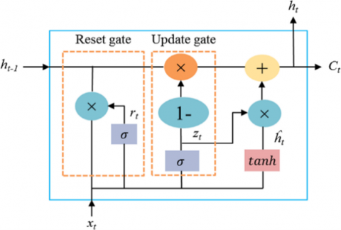
The structure of the GRU model is illustrated in Figure 1 [32].
The gates of the GRU model are defined by [33].
${{r}_{t}}=\sigma \left( {{W}_{r}}.{{x}_{t}}+{{U}_{r}}.{{h}_{t-1}}+{{b}_{r}} \right)$ (1)
${{z}_{t}}=\sigma \left( {{W}_{z}}.{{x}_{t}}+{{U}_{z}}.{{h}_{t-1}}+{{b}_{z}} \right)$ (2)
${{\tilde{h}}_{t}}=\tanh \left( {{W}_{h}}.{{x}_{t}}+{{U}_{h}}.\left( {{r}_{t}}\odot {{h}_{t-1}} \right)+{{b}_{h}} \right)$ (3)
${{h}_{t}}=\left( 1-{{z}_{t}} \right)\odot {{h}_{t-1}}+{{z}_{t}}{{\tilde{h}}_{t}}$ (4)
where $\mathrm{X}_{\mathrm{t}}-$ input vector at time step $t$; $\mathrm{h}_{\mathrm{t}-1}-$ hidden state at the previous time step; $\sigma-$ activation function; $\tanh -$ hyperbolic tangent activation function; $W_r, W_z, W_h$ and $\mathrm{U}_{\mathrm{r}}, \mathrm{U}_{\mathrm{z}}, \mathrm{U}_{\mathrm{h}}-$ weight matrices for each gate; $\mathrm{b}_{\mathrm{r}}, \mathrm{b}_{\mathrm{z}}, \mathrm{b}_{\mathrm{h}}-$ bias vectors associated with each gate. $\odot-$ denotes element-wise product.
Figure 1. Structure of GRU model
2.2 XGBoost model
The XGBoost algorithm can be regarded as an ensemble model consisting of $M$ decision trees, expressed as [14]:
${{\text{ }\!\!\Upsilon\!\!\text{ }}_{i}}=\underset{m=1}{\overset{M}{\mathop \sum }}\,{{f}_{m}}\left( {{x}_{i}} \right),~{{f}_{m}}\in F$ (5)
where, f denotes a decision tree and F represents the functional space of all decision trees. During regression, the objective function of the additive model is expressed as:
$b_j(\theta)=\sum_{i=1}^n l\left(y_i, \Upsilon_i\right)+\sum_{m=1}^M \Omega\left(f_m\right), \theta=\left(f_i\right)$ (6)
where, $l$ denotes the loss function and $\Omega$ represents the regularization term. A vector mapping is employed to enhance decision trees for each regularization term $\Omega(\mathrm{f})$. The regularization term can be expressed as:
$\text{ }\!\!\Omega\!\!\text{ }\left( f \right)=\gamma T+\frac{1}{2}\lambda \underset{j=1}{\overset{T}{\mathop \sum }}\,\omega _{j}^{2}$ (7)
where, $T$ denotes the number of leaf nodes of the decision tree, $\omega$ represents the weight vector of the leaf nodes, and both $\gamma$ and $\lambda$ are penalty coefficients. At the $t$ iteration, the predicted value of the sample $x_i$ is given by:
$\text{ }\!\!\Upsilon\!\!\text{ }_{i}^{t}=\text{ }\!\!\Upsilon\!\!\text{ }_{i}^{t-1}+{{f}_{t}}\left( {{x}_{i}} \right)$ (8)
Therefore, the objective function can be expressed as follows:
$\begin{aligned} & \operatorname{Obj}(\theta)^t=\sum_{i=1}^n l\left(y_i, \Upsilon_i^t\right)+\sum_{m=1}^t \Omega\left(f_m\right) \\ = & \sum_{i=1}^n l\left(y_i, Y_i^{t-1}+f_t\left(x_i\right)\right)+\sum_{m=1}^t \Omega\left(f_m\right)\end{aligned}$ (9)
The greedy algorithm is employed in XGBoost to construct decision trees iteratively, thereby forming a complete XGBoost model. In addition, a randomization technique is introduced to mitigate overfitting and accelerate the training process. Furthermore, XGBoost incorporates a sparsity-aware algorithm to efficiently handle missing values by excluding them from the loss gain computation of candidate splits.
2.3 Proposed model for wind power forecasting under data loss conditions
To leverage the advantages of fast training time, strong generalization capability, and robustness to noisy data of the GRU model, together with the ability of XGBoost to capture long-term temporal dependencies, this study proposes a hybrid forecasting framework that integrates XGBoost with GRU. In the context where wind power data may be missing at certain time steps, XGBoost is employed to interpolate the missing values rather than relying solely on the GRU model to perform sequential predictions. This approach is designed to mitigate the problem of error accumulation, which is commonly encountered in multi-step ahead forecasting with deep learning models. Specifically, the operational scheme of the proposed XGBoost-GRU model is illustrated as Figure 2.
Figure 2. XGBoost–GRU model for wind power forecasting under missing data conditions
In this study, the GRU model is configured to employ a fixed look-back window of 24 hours. This implies that, in order to forecast wind power at any given time, the model requires a continuous input sequence covering the preceding 24 hours. In other words, the time series data are restructured into pairs of input sequences and output target values. Specifically, to forecast the power at time $t$, the model utilizes an input vector sequence consisting of all data points from time $t-k$ to $t-1$, where $k=24$ denotes the look-back window length.
2.4 Evaluation and selection of forecasting models
After training, the models are evaluated using three primary performance metrics: Root Mean Square Error (RMSE), Mean Absolute Percentage Error (MAPE), and Normalized Mean Absolute Percentage Error (NMAPE). These error metrics are mathematically defined as follows [16, 24]:
RMSE $=\sqrt{\frac{1}{n} \sum_{\mathrm{i}=1}^{\mathrm{n}}\left(\hat{\mathrm{y}}_{\mathrm{i}}-\mathrm{y}_{\mathrm{i}}\right)^2}$ (10)
NRMSE $=\sqrt{\frac{1}{\mathrm{n}} \sum_{\mathrm{i}=1}^{\mathrm{n}} \frac{\left(\hat{y}_{\mathrm{i}}-\mathrm{y}_{\mathrm{i}}\right)^2}{\text { capacity }}}$ (11)
MAPE $=\frac{100}{\mathrm{n}} \sum_{\mathrm{i}=1}^{\mathrm{n}} \frac{\left|\mathrm{P}_{\mathrm{i}}^{\mathrm{db}}-\mathrm{P}_{\mathrm{i}}^{\mathrm{tt}}\right|}{\mathrm{P}_{\mathrm{i}}^{\mathrm{tt}}}$ (12)
NMAPE $=\frac{100}{\mathrm{n}} \sum_{\mathrm{i}=1}^{\mathrm{n}} \frac{\left|\mathrm{P}_{\mathrm{i}}^{\mathrm{db}}-\mathrm{P}_{\mathrm{i}}^{\mathrm{tt}}\right|}{\mathrm{P}_{\mathrm{dm}}}$ (13)
where: $\hat{\mathrm{y}}_{\mathrm{i}}-$ the predicted power output (kW), $\mathrm{y}_{\mathrm{i}}-$ the actual power output (kW), $P_i^{d b}-$ the predicted power generation (MW), $\mathrm{P}_{\mathrm{i}}^{\mathrm{tt}}-$ the actual power generation (MW), $\mathrm{P}_{\mathrm{dm}}-$ denotes the rated (installed) capacity of the power plant (MW), Capacity is the total installed capacity of the plant (kW), $\mathrm{n}-$ the number of forecasted instances evaluated within the considered forecasting period.
The output power $P(\mathrm{W})$ generated by each wind turbine can be expressed as follows [24]:
$\mathrm{P}=\frac{1}{2} \rho \cdot A \cdot C_p \cdot N_p \cdot N_g \cdot N_b \cdot V^3$ (14)
where, $\rho-$ the air density (kg/m3), A - the rotor swept area (m2), $C_p-$ the power coefficient, V - the wind speed (m/s), $\mathrm{Ng}-$ the generator efficiency, $\mathrm{N}_{\mathrm{b}}-$ the gearbox efficiency.
$\rho=\frac{353}{T+273} e^{\frac{-h}{29.3(T+273)}}$ (15)
In this study, the forecasting dataset was obtained from the Supervisory Control and Data Acquisition (SCADA) system of the Ninh Thuan Wind Farm. The data collection spanned a period of 360 days, from January 1, 2024, to December 31, 2024. Measurements were continuously recorded at 30-minute intervals, 24 hours per day, from turbine WT01 with a rated capacity of 4 MW. Accordingly, each day comprised 144 data samples. Each sample contained the following input features: power output, wind speed, rotor speed, pitch angle, vibration level, and internal temperature. The dataset for one year is represented in the format month/day/hour:minute, with the characteristic parameters summarized in Table 1. Two representative days, January 1, 2024, and December 31, 2024, are illustrated, while the remaining days follow the same structure.
Table 1. Structure of the collected dataset with a 30-minute sampling interval
|
Date Time |
Wind Speed |
Power Output |
Rotor Speed |
Pitch Angle |
Vibration Level |
Internal Temp |
|
01/01/2024/0:00 |
3.84 |
182.08 |
5.71 |
0 |
0.13 |
15.38 |
|
01/01/2024/0:30 |
5.39 |
650.5 |
7.33 |
0 |
0.13 |
16.7 |
|
01/01/2024/1:00 |
4.43 |
229.3 |
5.96 |
0.11 |
0.11 |
15.2 |
|
01/01/2024/1:30 |
5.24 |
601.67 |
7.59 |
0.41 |
0.07 |
17.23 |
|
…… |
…… |
…… |
…… |
…… |
…… |
…… |
|
12/31/2024/22:00 |
2.96 |
0 |
4.32 |
0 |
0.07 |
19.66 |
|
12/31/2024/22:30 |
2.45 |
0 |
3.29 |
0 |
0.13 |
18.12 |
|
12/31/2024/23:00 |
1.96 |
0 |
3.48 |
0 |
0.09 |
15.35 |
|
12/31/2024/23:30 |
4.73 |
385.75 |
6.36 |
0 |
0.1 |
16.96 |
The dataset employed for model development was sampled at 30-minute intervals and subsequently divided into training and testing subsets, with 70% allocated for training and 30% reserved for testing. In addition, an independent forecasting dataset, covering the period from February 1 to February 3, 2025, was constructed and excluded from the training phase to evaluate the generalization capability of the proposed model. After preprocessing, the dataset achieved a fit accuracy of 0.98, and its distribution is illustrated in Figure 3.
Figure 3. Wind data distribution
Experimental results were obtained using the proposed XGBoost-GRU hybrid model for the forecasting period from March 1 to March 3, 2024. The performance of the ensemble model was compared against the standalone GRU model under conditions of missing historical input data. The evaluation scenarios were designed based on the absolute duration of missing data within the 24-hour lookback window, and are defined as follows:
- Baseline scenario: No missing data is introduced.
- Short interruption scenario: Random data segments with a cumulative length of 2 hours and 6 hours are removed.
- Medium interruption scenario: A continuous data segment of 12 hours (equivalent to half of the lookback window) is removed.
- Total interruption scenario: All data within the 24-hour lookback window is removed.
- Extreme outage scenario: A 28-hour data segment-longer than the lookback window itself-is removed to assess the model’s fault tolerance and its operational failure threshold.
The mechanism of missing data, as described above, reflects practical operating conditions in wind farms, where measurement device failures, network errors, or power outages may occur.
In the proposed XGBoost-GRU model, the lookback parameter is set to 48 with a data sampling frequency of 30 minutes. Accordingly, the lookback window corresponds to a 24-hour period (48 steps × 30 minutes/step). For instance, to forecast the power output at 15:00 on March 2, the GRU component requires a complete sequence of 48 consecutive power values, ranging from 15:00 on March 1 to 14:30 on March 2.
After generating the forecast for 15:00, the lookback window is shifted forward by one step. Thus, the subsequent forecast at 15:30 requires the sequence from 15:30 on March 1 to 15:00 on March 2. This sliding-window mechanism is repeated across the entire forecasting horizon. By leveraging the lookback window, the model is capable of capturing not only instantaneous variations but also temporal dependencies such as trends, cyclic patterns (e.g., diurnal cycles), and momentum in the time series, which are critical for achieving accurate forecasting results.
Comparison Methods: In each missing-data scenario, the forecasting performance of two approaches is compared:
- Baseline GRU model: Missing data points within the lookback window are replaced with zero values.
- XGBoost-GRU hybrid model: An XGBoost-based interpolation module is employed to estimate and impute the missing values before the reconstructed sequence is provided to the GRU forecaster.
Hyperparameters of the XGBoost model Number of Trees: 500 trees Learning Rate: 0.05 Maximum Tree Depth: 5 leaves Objective Function: Mean Squared Error for regression. Parallel Processing: Uses all available CPU cores Hyperparameters of the GRU model First GRU Layer: Number of Neurons: 100 First Dropout Layer: Dropout Rate: 20% Second GRU Layer: Number of Neurons: 100 Second Dropout Layer: Dropout Rate: 20% Dense (Output) Layer: Number of Neurons: 1 (to predict a single value) Training configuration of GRU: Optimizer: adam Loss function: mean_squared_error (MSE) Epochs: 50 used with EarlyStopping to avoid overfitting batch size: 64.
The evaluation is conducted on the entire forecast dataset using a stepwise validation strategy, which closely mimics real-world operational forecasting. Performance is assessed using error metrics such as the Root Mean Square Error (RMSE) and the Mean Absolute Error (MAE), recorded for each scenario. To validate the suitability of the proposed XGBoost–GRU model for wind power forecasting under missing data conditions, a comparative analysis with the Long Short-Term Memory (LSTM) model is conducted under the same conditions. The comparative results of the forecasting models under missing-data conditions are summarized in Table 2.
Table 2. Evaluation results: 1- GRU (No inputation); 2- XGBoost-GRU; 3 - LSTM (No inputation)
|
Script |
Case |
RMSE (kW) |
MAPE (kW) |
NRMSE (%) |
NMAPE (%) |
|
Full data |
1 |
671.55 |
526.6 |
16.79 |
13.17 |
|
2 |
671.55 |
526.6 |
16.79 |
13.17 |
|
|
3 |
670.37 |
525.1 |
16.76 |
13.13 |
|
|
Missing data 2h |
1 |
708.74 |
540.52 |
17.72 |
13.51 |
|
2 |
671.68 |
526.72 |
16.79 |
13.17 |
|
|
3 |
691.89 |
533 |
17.3 |
13.33 |
|
|
Missing data 6h |
1 |
740.86 |
557.43 |
18.52 |
13.94 |
|
2 |
672.4 |
527.55 |
16.81 |
13.19 |
|
|
3 |
726.16 |
551.99 |
18.15 |
13.8 |
|
|
Missing data 9h |
1 |
799.31 |
597.2 |
19.98 |
14.93 |
|
2 |
671.54 |
526.6 |
16.79 |
13.17 |
|
|
3 |
771.97 |
580.39 |
19.3 |
14.51 |
|
|
Missing data 12h |
1 |
937.3 |
711.67 |
23.43 |
17.79 |
|
2 |
672.1 |
527.28 |
16.8 |
13.18 |
|
|
3 |
874.64 |
646.27 |
21.87 |
16.16 |
|
|
Missing data 24h |
1 |
1282.64 |
1070.12 |
32.07 |
26.75 |
|
2 |
671.92 |
526.96 |
16.8 |
13.17 |
|
|
3 |
1112.54 |
875.85 |
27.81 |
21.9 |
|
|
Missing data 28h |
1 |
1282.64 |
1070.12 |
32.07 |
26.75 |
|
2 |
671.92 |
526.96 |
16.8 |
13.17 |
|
|
3 |
1112.54 |
875.85 |
27.81 |
21.9 |
Table 2 highlights the significant performance differences between the forecasting models under missing-data conditions. The standalone GRU model, when deprived of recent historical sequences, exhibits severe performance degradation. Specifically, the model reports an RMSE of 1282.64kW, an NRMSE of 32.07%, and a MAPE of 26.75% when the missing-data period extends beyond 24 hours.
In contrast, under the ideal scenario with complete historical data available from February 15 to February 28, the GRU model achieves substantially lower errors, with an RMSE of 671.55 kW, an NRMSE of 16.79%, and a MAPE of 13.17%.
The LSTM model outperforms the GRU model, achieving an RMSE of 1112.54 kW, an NRMSE of 27.81%, and a MAPE of 21.9% when the missing-data period exceeds 24 hours.
Most notably, when the XGBoost–GRU hybrid approach is employed to interpolate missing values before forecasting, the model demonstrates robust fault tolerance and stable performance. The results show that the hybrid approach achieves RMSE = 671.92kW, NRMSE = 16.8%, and MAPE = 13.17%, which are very close to the ideal scenario despite the missing-data condition.
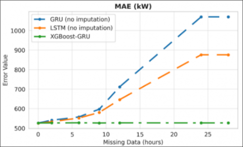
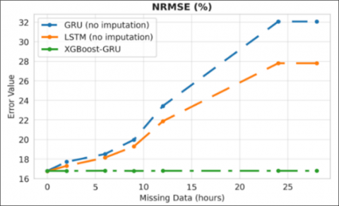
To further illustrate the error behavior across different scenarios, Figure 4 depicts the comparative error distribution of the standalone GRU model versus the XGBoost-GRU hybrid model and LSTM model when handling incomplete time series inputs.
The results in Figure 4 indicate a clear contrast in error dynamics between the two approaches. For the standalone GRU model and LSTM model, the forecasting error increases progressively as the duration of missing data extends from 2 to 24 hours. Beyond this point, however, the error no longer grows; instead, it saturates at a consistently high level. In other words, when the missing-data window exceeds 24 hours (e.g., in the 28-hour scenario), the error indices remain nearly constant, reflecting the model’s performance ceiling.
This phenomenon can be interpreted as the appearance of an error saturation threshold for the base GRU, LSTM model. Once the missing duration surpasses the look-back horizon, the model’s input sequence degenerates into a constant vector (filled with zeros). Consequently, the model loses all temporal dependencies and meaningful patterns, producing stationary forecasts and yielding stable but high errors. This aligns with the “Garbage In, Garbage Out” principle, emphasizing the model’s inability to recover useful information when deprived of adequate historical data.
(a) The RMSE under time missing data conditions
(b) The MAE under time missing data conditions
(c) The NRMSE under time missing data conditions
(d) The NMAPE under time missing data conditions
Figure 4. Error in case of GRU, XGBoost-GRU and LSTM
By contrast, the hybrid XGBoost-GRU approach demonstrates strong resilience. Its error values remain stable and closely aligned with those of the ideal scenario (no missing data), regardless of the duration of the missing interval. This highlights the effectiveness of the interpolation step in reconstructing informative input sequences and preventing the error saturation observed in the baseline GRU, LSTM.
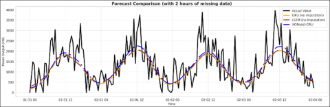
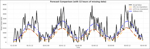
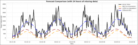
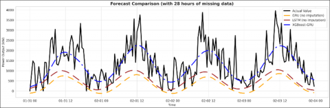
Figure 5 compares the forecasted power outputs under different conditions of missing historical data as defined in the proposed scenarios.
(a) The output power under full data conditions
(b) The output power under 2-hour missing data conditions
(c) The output power under 6-hour missing data conditions
(d) The output power under 9-hour missing data conditions
(e) The output power under 12-hour missing data conditions
(f) The output power under 24-hour missing data conditions
(g) The output power under 28-hour missing data conditions
Figure 5. Comparison of transmission power forecast of XGBoost- GRU, GRU and LSTM models
Figure 5 illustrates that, in the case of complete input data, both the GRU, LSTM and XGBoost–GRU models are able to closely follow the actual power output. However, when the amount of missing data increases from 2 hours up to 28 hours, the standalone GRU, LSTM model gradually loses its ability to learn and reproduce the underlying trend, resulting in significantly larger forecasting errors. In contrast, the hybrid XGBoost–GRU model, by applying a guided interpolation process to reconstruct a sufficiently long input sequence before feeding it into the GRU, consistently maintains stable and accurate tracking of the actual data. These results confirm that incorporating XGBoost for missing data reconstruction effectively restores the input sequence, thereby preserving the learning capability of the GRU deep sequence model.
The experimental results demonstrate that the hybrid XGBoost-GRU model consistently outperforms the baseline GRU model across all missing data scenarios. As the proportion of missing data increases, the forecasting error of the baseline GRU model grows exponentially, whereas the hybrid model maintains relatively stable accuracy.
A notable finding is the emergence of an error saturation threshold for the baseline GRU model. Specifically, when the duration of missing data reaches or exceeds 24 hours (e.g., in the 28-hour scenario), the error metrics of this model no longer increase but instead remain at a very high and nearly constant level, indicating that the model has reached its operational limit. This error saturation phenomenon can be explained by the “Garbage In, Garbage Out” principle. Once the missing data exceeds the look-back window, the input to the baseline GRU degenerates into a constant vector sequence (all zero values). Consequently, the model loses its ability to extract meaningful information, and its forecasts become stationary, leading to constant errors. This behavior does not imply underfitting during training; rather, it represents an inference failure caused by meaningless input.
In contrast, the ability of the XGBoost interpolation model to provide a more meaningful input sequence enables the GRU model to avoid complete failure, thereby demonstrating the robustness and reliability of the hybrid approach.
This study highlights two key findings: (1) The integration of an intelligent interpolation model such as XGBoost is an effective strategy that significantly enhances the accuracy and resilience of time-series forecasting models under incomplete data conditions. (2) The study identifies and explains the critical failure threshold of regression-based models when confronted with large data gaps, emphasizing the importance of properly handling missing data in practical applications.
This study also highlights the potential for practical deployment in wind farms. To ensure feasibility in real-world applications, the XGBoost–GRU model must satisfy real-time requirements, particularly in updating and processing forecast data with low latency. Integration on GPU-based platforms or edge servers can further enhance processing speed and optimize operational costs.
This work was partially supported by: 1. Hanoi University of Mining and Geology; 2. Hue University under the Core Research Program, Grant No. NCTB.DHH.2024.08.
[1] Biswal, B., Deb, S., Datta, S., Ustun, T.S., Cali, U. (2024). Review on smart grid load forecasting for smart energy management using machine learning and deep learning techniques. Energy Reports, 12: 3654-3670. https://doi.org/10.1016/j.egyr.2024.09.056
[2] Hong, N.T., Vuong, D.Q., Cuong, N.X., Do, N.Y. (2023). Long-term performance of roof-top GCPV systems in central Viet Nam. International Journal of Renewable Energy Development, 12(6): 998-1007. https://doi.org/10.14710/ijred.2023.56569
[3] Liu, L., Wang, J. (2021). Super multi-step wind speed forecasting system with training set extension and horizontal–vertical integration neural network. Applied Energy, 292: 116908. https://doi.org/10.1016/j.apenergy.2021.116908
[4] Liu, L., Wang, J. (2021). A two-stage deep autoencoder-based missing data imputation method for wind farm SCADA data. IEEE Sensors Journal, 21(9): 10933-10945. https://doi.org/10.1109/JSEN.2021.3061109
[5] Cuong, N.X., Do, N.Y., Vuong, D.Q. (2022). Modeling and experimental studies on water spray cooler for commercial photovoltaic modules. International Journal of Renewable Energy Development, 11(4): 926-935. https://doi.org/10.14710/ijred.2022.46209
[6] Surucu, O., Gadsden, S.A., Yawney, J. (2023). condition monitoring using machine learning: A review of theory, applications, and recent advances. Expert Systems with Applications, 221: 119738. https://doi.org/10.1016/j.eswa.2023.119738
[7] Tawn, R., Browell, J., Dinwoodie, I. (2020). Missing data in wind farm time series: Properties and effect on forecasts. Electric Power Systems Research, 189: 106640. https://doi.org/10.1016/j.epsr.2020.106640
[8] Liu, T., Wei, H., Zhang, K. (2018). Wind power prediction with missing data using Gaussian process regression and multiple imputation. Applied Soft Computing, 71: 905-916. https://doi.org/10.1016/j.asoc.2018.07.027
[9] Hui, H.G., Chunyang, D., Wei, D., Daiyu, X., Fangjun, W., Li, K., Xia, W. (2023). A hybrid short-term wind power forecasting model considering significant data loss. Transactions on Electrical and Electronic Engineering, 19(3): 349-361. https://doi.org/10.1002/tee.23970
[10] Wei, W., Jian, Y., Yihuan, L., Guorui, R., Kang, L. (2025). Data-driven deep learning model for short-term wind power prediction assisted with WGAN-GP data preprocessing. Expert Systems with Applications, 275: 127068. https://doi.org/10.1016/j.eswa.2025.127068
[11] Ting, Y., Zhenning, Y., Fei, L., Hengyu, W. (2024). A short-term wind power forecasting method based on multivariate signal decomposition and variable selection. Applied Energy, 360: 122759. https://doi.org/10.1016/j.apenergy.2024.122759
[12] Zheng, L., Ruosi, X., Xiaorui, L., Xin, C., Hexu, S. (2023). Short-term wind power prediction based on modal reconstruction and CNN-BiLSTM. Energy Reports, 9: 6449-6460. https://doi.org/10.1016/j.egyr.2023.06.005
[13] Yu, L., Fei, T., Xin, G., Tongyan, Z., Junfeng, Q., Jiarui, X., Xinang, L., Yuhan, G. (2022). Numerical weather prediction correction strategy for short-term wind power forecasting based on bidirectional gated recurrent unit and XGBoost. Frontiers in Energy Research, 9: 1-14. https://doi.org/10.3389/fenrg.2021.836144
[14] Quoc, T.P., Yuan, K.W., Quoc, D.P. (2021). A hybrid wind power forecasting model with XGBoost, data preprocessing considering different NWPs. Applied Sciences, 11(3): 1000. https://doi.org/10.3390/app11031100
[15] Yang, L., Ruinong, W., Meng, Z., Chao, L. (2023). Wind power forecasting considering data privacy protection: A federated deep reinforcement learning approach. Applied Energy, 329: 120291. https://doi.org/10.1016/j.apenergy.2022.120291
[16] Liu, Z., Guo, H., Zhang, Y., Zuo, Z. (2021). A comprehensive review of wind power prediction based on machine learning: models, applications, and challenges. Energies, 18(2): 350. https://doi.org/10.3390/en18020350
[17] Prema, V., Bhaskar, M.S., Dhafer, A., Gowtham, N., Uma, R.K. (2025). Critical review of data, models and performance metrics for wind and solar power forecast. IEEE Access, 10: 667-688. https://doi.org/10.1109/ACCESS.2021.3137419
[18] Tan, H., Lin, S., Xu, X., Shi, P., Li, R., Wang, S. (2023). Missing data recovery of wind speed in wind farms: A spatial-temporal tensor decomposition approach. Journal of Renewable and Sustainable Energy, 15(3): 033302. https://doi.org/10.1063/5.0144648
[19] Akçay, H., Filik, T. (2017). Short-term wind speed forecasting by spectral analysis from long-term observations with missing values. Applied Energy, 191: 653-662. https://doi.org/10.1016/j.apenergy.2017.01.063
[20] Jiang, H., Wu, A., Wang, B., Xu, P., Yao, G. (2020). Industrial ultra-short-term load forecasting with data completion. IEEE Access, 8: 158928-158940. https://doi.org/10.1109/ACCESS.2020.3017655
[21] Chen, J., Wei, Z., Zhang, J. (2025). A hybrid neural network for the traffic flow prediction on the premise of missing data. IET Intelligent Transport Systems, 19(1): e70070. https://doi.org/10.1049/itr2.70070
[22] Namrye, S., Seunghak, Y., Jeongseung, N. (2019). Hybrid forecasting model for short-term wind power prediction using modified long short-term memor. Energies, 12(20): 3901. https://doi.org/10.3390/en12203901
[23] Krishna, M.Y., Aluri, R., Rama, S.K. (2025). Hybrid machine learning models for wind power forecasting: A comparative analysis of support vector machine-arima and random Forest-XG boost. IICTCS 2024. Lecture Notes in Networks and Systems, 1384: 363-377. https://doi.org/10.1007/978-981-96-5751-3_31
[24] Guana, S., Wanga, Y., Liua, L., Gao, J., Xua, Z., Kand, S. (2023). Ultra-short-term wind power prediction method combining financial technology feature engineering and XGBoost algorithm. Heliyon, 9(6): e16938. https://doi.org/10.1016/j.heliyon.2023.e16938
[25] Mehmet, B., Emrah, D., Ugur, Y. (2025). A hybrid lstm-single candidate optimizer model for short-term wind power prediction. Computer Modeling in Engineering and Sciences, 144(1): 945-968. https://doi.org/10.32604/cmes.2025.067851
[26] Ally, S., Verstraeten, T., Daems, P., Nowé, A., Helsen, J. (2025). Modular deep learning approach for wind farm power forecasting and wake loss prediction. Wind Energy Science, 10(4): 779-812. https://doi.org/10.5194/wes-10-779-2025
[27] Namal, R., Jeevani, J., Rashmi, S., Upaka, R. (2025). Predicting short-term wind power generation at Musalpetti wind farm: Model development and analysis. Computer Modeling in Engineering and Sciences, 143(2): 2287-2305. https://doi.org/10.32604/cmes.2025.064464
[28] Wu, N.J., Hsu, T.W., Lin, T.C. (2025). A pattern-based machine learning model for imputing missing records in coastal wind observation networks. Meteorological Applications, 143(2): e70050. https://doi.org/10.1002/met.70050
[29] Ngo, X.C., Nguyen, T.H., Do, N.Y., Nguyen, D.M., et al. (2020). Grid-connected photovoltaic systems with single-axis sun tracker: Case study for central Vietnam. Energies, 13(6): 1457. https://doi.org/10.3390/en13061457
[30] Nehal, E., Haytham, E. (2025). Wind speed and power forecasting using Bayesian optimized machine learning models in Gabal Al-Zayt, Egypt. Scientific Reports, 15(1): 28500. https://doi.org/10.1038/s41598-025-13140-x
[31] Javier, S.S., Pedro, J.P.F., Carlos, Q.G.M.Q. (2025). Historical hourly information of four european wind farms for wind energy forecasting and maintenance. Data, 10(3): 38. https://doi.org/10.3390/data10030038
[32] Mohsen, S. (2023). Recognition of human activity using GRU deep learning algorithm. Multimedia Tools and Applications, 82(30): 47733-47749. https://doi.org/10.1007/s11042-023-15571-y
[33] Rial, A.R., Raden, A.A.R., Lee, H.L. (2020). A review on deep learning models for forecasting time series data of solar irradiance and photovoltaic power. Energies, 13(24): 6623. https://doi.org/10.3390/en13246623