Nourredine Tadj![]() | Djekidel Rabah*
| Djekidel Rabah*![]() | Abdechafik Hadjadj
| Abdechafik Hadjadj![]() | Bessidik Sid Ahmed
| Bessidik Sid Ahmed![]() | Takieddine Meriouma
| Takieddine Meriouma![]()
© 2025 The authors. This article is published by IIETA and is licensed under the CC BY 4.0 license (http://creativecommons.org/licenses/by/4.0/).
OPEN ACCESS
The permanent presence of metallic pipelines in the soil produces electrochemical reactions, which leads to the corrosion activity and thus, an adequate cathodic protection strategy is required. The purpose of this paper is to assess the effect of inductive coupling between an EHV overhead power line and a buried metallic pipeline in normal operation; and to optimize a sacrificial anode cathodic protection system from corrosion evolution using a new efficient meta-heuristic algorithm of Teaching Learning Based Optimization (TLBO). The results obtained indicate that the induced voltage resulting from the inductive coupling exceeds the limit recommended by the majority of international standards; the calculated value of corrosion current density presents a relevant parameter having a significant effect on the corrosion rate and metal loss. Therefore; the selected optimization algorithm proves to be accurate in determining the parameters associated with the design of the sacrificial anode cathodic protection system and is able to meet the current requirement criterion necessary for the protection implemented and to ensure the stability and optimal performance of the hydrocarbon transportation pipeline system.
algorithm, buried metallic pipeline, sacrificial anode cathodic protection, corrosion, EHV overhead power line, inductive coupling, Teaching Learning Based Optimization (TLBO)
Metallic pipelines used for hydrocarbon transportation play a crucial role in the economies of countries that produce energy resources. Rising electricity demand in developing countries has intensified the need for energy supplies, especially since both types of transportation systems operate over extended distances to meet their operational requirements [1, 2].
However, sharing a common right of way is inevitable, which leads to the presence of the electromagnetic mutual interference problem. In the normal operation of overhead power lines of electricity transmission at higher voltage levels, this mutual interference can cause through inductive coupling in a parallel zone a development of an induced electrical potential in the metallic pipelines by the phenomenon of electromagnetic induction, which means that the magnetic field fluctuation caused by three-phase power flow through the conductors of elevated high voltage electrical networks contributes to the generation of electromotive forces between the buried pipeline and the nearby soil, and consequently the circulation of AC induced current between the ends of the metallic pipeline, which can present risks of electric shock for maintenance operators and steel corrosion [3-6].
The term corrosion refers to a process that causes the progressive deterioration of the metal constituting the pipelines due to electrochemical reactions on the surface of the metal with its environment, this leads to a reduction in the progressive thinning of the metal, quantified by the amount of mass lost per area over time [7]. In order to increase the operational life and protect steel pipelines potentially subjected to corrosive action, two types of complementary protections are combined with each other to ensure effective protection of pipelines. Firstly, the passive protection by covering the outer surface of the buried pipeline with an insulating organic layer of a certain thickness, often consisting of bituminous, epoxy and polymers. Secondly, the cathodic protection which consists of connecting an external anode is connected to the buried pipeline, enabling current flow that ensures the entire structure remains cathodic, thereby preventing any form of corrosion. There are generally two types of cathodic protection, sacrificial anode protection where the protection current comes from a metal whose corrosion potential is more negative than that of the pipeline metal to be protected, and impressed current protection in which the DC direct current is provided by an external generator supplying a more or less inert auxiliary anode called "groundbed" [7-11]. The first use of cathodic protection dates back to 1824, when Humphry Davy protected copper structures of British ships from marine corrosion using iron anodes. Its use subsequently spread to the United States and England to meet the needs of economic and industrial development, encompassing various sectors, including metallic pipelines for the transport of oil, gas, and petrochemicals. The first use of impressed current cathodic protection for safeguarding buried structures was introduced in England and the United States during the period from 1910 to 1912. The rapid development of cathodic protection systems began in 1945 in the United States and England, in response to the demands of rapid economic and industrial development that included various sectors, such as the oil and gas industry, which was expanding and widespread at that time, and metallic pipelines were used in most oil, gas, and petrochemical transportation operations. The advantages of using thin, highly corrosion-resistant steel tubes in buried pipelines were exploited [12, 13]. Currently, cathodic protection is widely used in various industrial applications, mainly steel pipelines buried in the ground or submerged in water, water reservoirs, port structures and offshore platforms and ship hulls. Extensive research efforts encompassing experimental investigations, analytical modeling, and numerical simulations have been dedicated to understanding the phenomena of AC induced corrosion and optimizing cathodic protection systems. Over the past decades, a wide range of experimental, analytical, and computational studies has been carried out to deepen the understanding of AC corrosion mechanisms and the underlying principles of cathodic protection. These investigations have considered various influencing parameters, such as soil resistivity, current density, corrosion rate, and the physical and electrical characteristics of coating materials, all of which affect the overall effectiveness of protection systems. Altogether, these studies have greatly improved our understanding of the key factors that initiate and intensify AC corrosion in metallic pipelines, and have contributed to the development of more effective and reliable cathodic protection approaches.
Based on this research, several internationally recognized standards, such as NACE-0169, NF-EN-12954, and DNV-RP-B401, have been established to guide the reliable and efficient protection of metallic structures. Moreover, recent progress in Artificial Intelligence (AI) and Evolutionary Optimization (EO) techniques has significantly enhanced the design, efficiency, and adaptability of cathodic protection systems [14-17]. Despite the double protection of steel pipelines, in case where the buried pipelines are located extra-high-voltage power lines with high alternating current, failure and corrosion cracking on the metal surface may occur as a result of pipeline coating defects, causing a significant disruption in the normal operation of pipeline systems. The major concern of hydrocarbon transmission and distribution network operators is to ensure the maintenance and integrity of the entire pipeline to ensure safe and reliable operation throughout its longevity and to keep the safety of intervention agents [18-26].
This study investigates the inductive coupling between an overhead extra-high-voltage AC transmission line and a nearby buried metallic pipeline, based on the lossy transmission line theory and electromagnetic induction principles. It assesses the induced voltage amplitude and the main parameters influencing AC corrosion along the buried pipeline. To mitigate these effects, an optimized cathodic protection system using sacrificial anodes is designed and installed, with its optimization performed through a recent algorithm known as TLBO. Determining the AC current density flowing between the pipeline and the surrounding soil and the instantaneous rate of metal corrosion present fundamental criteria for the probability of AC induced corrosion levels; in order to design a well-adapted preventive measure aimed at eliminating corrosion risks. A cathodic protection system can be designed and optimized using a sacrificial anode to properly protect metallic pipelines from AC corrosion. The optimization tool used is based on a social communication inspired algorithm called TLBO. TLBO is a new stochastic and global optimization technique, this strategy, introduced by Rao et al. [27], is conceptually inspired by the natural process of knowledge transfer in education, particularly focusing on how instructors shape student development. This algorithm has proven to be very reliable and robust in finding the ideal values of the search parameters, it has been successfully applied in several industrial applications.
While a buried pipeline and an overhead power line are sharing same corridor, magnetic coupling occurs under normal operating conditions as well as during a fault. Inductive interference is the result of the time-varying magnetic field produced by the currents flowing in the conductors of the transmission line, the buried metallic pipeline installed nearby is subject to the appearance of an induced voltage relative to the ground immediately surrounding it and an induced current flowing in it. This phenomenon expresses the laws of electromagnetic induction of Faraday and Lenz, whose mechanism can be represented by an electric transformer where the power line represents the primary coil and the pipeline acts as a secondary coil [28-34]. Based on Biot and Savart's law, the magnetic induction at a point M in space, caused by a current flowing through an infinitely long straight conductor, can be expressed as follows [28]:
${{B}_{T}}=\text{ }\frac{{{\mu }_{0}}}{2\pi }\frac{I}{d}$ (1)
where,$~I$ is the current flowing in the electrical conductor; $d$ is the distance between the conductor and the location M where the magnetic field is evaluated;$~{{\mu }_{0}}$ is the permeability of free space.
The magnetic flux induced by the alternating currents in the power line conductors is determined by performing a surface integral of the magnetic field across the loop space formed by the pipeline circuit; as indicated in the equation below [28]:
${{\varphi }_{T}}=\int\limits_{S}{{{B}_{T}}dS}$ (2)
Figure 1 illustrates the coordinates of the arrangement of the electrical transmission conductors and the adjacent underground pipeline. Since the plane of the pipeline loop is perpendicular to the ground surface, only the horizontal component of the magnetic field is perpendicular to the plane of the buried pipeline. The resulting total magnetic flux, which is obtained by integrating the previous equation, is expressed by the following relationship [28-34]:
${{\varphi }_{T}}=\frac{{{\mu }_{0}}\,\,}{4\,\pi }\sum\limits_{i=1}^{n}{{{I}_{i}}}\ln \left[ \frac{{{\left( {{x}_{p}}-{{x}_{i}} \right)}^{2}}+{{\left( {{y}_{p}}+{{y}_{i}}+{{D}_{e}} \right)}^{2}}}{{{\left( {{x}_{p}}-{{x}_{i}} \right)}^{2}}+{{\left( {{y}_{p}}-{{y}_{i}} \right)}^{2}}} \right]$ (3)
where,$\text{ }\!\!~\!\!\text{ }{{\text{I}}_{\text{i}}}$ represents the current in the ith overhead conductor, and$\text{n}$indicates the total number of conductors. The coordinates $({{\text{x}}_{\text{i},}}\text{ }\!\!~\!\!\text{ }{{\text{y}}_{\text{i}}})$ specify the locations of the transmission power line conductors, whereas$\text{ }\!\!~\!\!\text{ }({{\text{x}}_{\text{j},}}\text{ }\!\!~\!\!\text{ }{{\text{y}}_{\text{j}}})\text{ }\!\!~\!\!\text{ }$denote the spatial position of the subterranean steel pipeline. The parameter ${{\text{D}}_{\text{e }\!\!~\!\!\text{ }}}$ corresponds to the complex penetration depth of the magnetic field into the conductive subsoil.
Figure 1. Evaluation of magnetic induction intensity resulting from an overhead conductor
The depth of penetration into the soil assumed to be perfectly conductive earth, which reflects the return path of the ground currents, can be obtained from the following mathematical expression:
${{D}_{e}}=658.87\sqrt{\frac{{{\rho }_{s}}}{f}}$ (4)
where,$~{{\rho }_{s}}$ is the electrical resistivity of the ground; $f$ represents the frequency of the power source current.
According to Faraday's law, the induced electromotive force on the parallel subterranean steel pipeline can be expressed by the following equation [28-34]:
${{E}_{ind}}=-\frac{d{{\phi }_{T}}}{dt}=-j\omega \,{{\varphi }_{T}}$ (5)
where,$~\omega $ is the angular power frequency, ${{\varphi }_{T}}$ is the total magnetic flux obtained in the previous equation. The negative sign in the equation reflects Lenz's law, which indicates that the induced electromotive force opposes the cause that produces it, which is the variation of the magnetic flux.
Indeed, to evaluate the induced voltage in the subterranean steel pipeline resulting from inductive coupling, the electrical behavior of the pipeline segment can be modeled using a lossy transmission line with π equivalent circuit, as illustrated in Figure 2. This electrical modeling is based on the equations of the telegraphists that permit to describe the evolution of the voltage and current in any position along the subterranean pipeline [28-34]. The equivalent electrical circuit modeling an underground steel pipeline section of length L relative to the ground, in parallel with an overhead power conductor between points (x = 0) and (x = L), can be considered as a combination of a series impedance and a parallel admittance of the buried pipeline system, as explained in Figure 2 below [28-34].
Figure 2. Modeling the electrical coupling between a buried pipeline and ground
From Figure 2, the equations that govern the evolution of the voltage and current at each point of the subterranean pipeline can be presented as below [28-34]:
$\frac{dV(x)}{dx}=-zI(x)+E(x)$ (6)
$\frac{dI(x)}{dx}=-yV(x)$ (7)
Upon applying differentiation with respect to the variable x indicating the longitudinal position and combining the resulting system equations, the analytical solution describing the distribution of electromotive force and electrical current along the underground steel pipeline is derived, as demonstrated by the two equations below [28-34]:
${{V}_{ind}}(x)=\frac{{{E}_{ind}}}{2\gamma }\left( {{e}^{\gamma \left( x-L \right)}}-{{e}^{-\gamma x}} \right)$ (8)
${{I}_{ind}}(x)=\frac{{{E}_{ind}}}{2{{Z}_{c}}}\left( 2-{{e}^{\gamma \left( x-L \right)}}-{{e}^{-\gamma x}} \right)$ (9)
where, $\text{x}$ and $\text{L}$ represent the both endpoints of the pipeline segment; $\text{ }\!\!\gamma\!\!\text{ }$ is the complex propagation factor describing the wave propagation along the underground pipeline; and ${{\text{Z}}_{\text{c}}}$ denotes the impedance’s characteristic. These two parameters are defined respectively as follows [28-34]:
$\left\{ \begin{align} & \gamma =\sqrt{zy} \\ & {{Z}_{c}}=\sqrt{{}^{z}/{}_{y}} \\ \end{align} \right.$ (10)
The series impedance per unit length with return to earth of the buried pipeline is given by the relation [28-34]:
$z=\frac{\sqrt{{{\rho }_{p}}{{\mu }_{p}}{{\mu }_{0}}\omega }}{\sqrt{2}\pi {{D}_{p}}}+\frac{{{\mu }_{0}}\omega }{8}+j\left[ \begin{align} & \frac{\sqrt{{{\rho }_{p}}{{\mu }_{p}}{{\mu }_{0}}\omega }}{\sqrt{2}\pi {{D}_{p}}}+\frac{{{\mu }_{0}}\omega }{2\pi } \\ & \times \ln (\frac{3.7\sqrt{{{\rho }_{s}}{{\omega }^{-1}}\mu _{0}^{-1}}}{{{D}_{p}}}) \\ \end{align} \right]$ (11)
where, Dp denotes the diameter of the subterranean pipeline, μp is the relative magnetic permeability of the pipeline material, and ρp represents the electrical resistivity of the subterranean steel pipeline.
The equivalent parallel admittance per unit length between the subterranean pipeline and the immediate soil is established by the following formula [28-34]:
$y=\frac{\pi {{D}_{p}}}{{{\rho }_{c}}{{\delta }_{c}}}+j\omega \frac{{{\varepsilon }_{0}}{{\varepsilon }_{r}}\pi {{D}_{p}}}{{{\delta }_{c}}}$ (12)
where,$\text{ }\!\!~\!\!\text{ }{{\text{ }\!\!\rho\!\!\text{ }}_{\text{c}}}$ represents the resistivity of the protective coating material, ${{\text{ }\!\!\varepsilon\!\!\text{ }}_{\text{r}}}$ designates the relative dielectric constant of the coating material and δc indicates the thickness of the applied outer coating layer.
Corrosion is a natural and destructive process by which metal gradually deteriorates due to electrochemical reactions with its surrounding environment. During this process, the metal tends to return to its original state of stability, often leading to damage and a loss of its essential properties. On the surface of the metal, corrosion typically involves at least two simultaneous chemical reactions [35-38]. The most common example in corrosion is the formation of rust on steel, which is mainly made of iron, with a low carbon amount and is widely used in pipeline construction. When iron corrodes, it forms rust through a reaction involving the reduction of oxygen and the dissolution of iron. This can be summarized by the following overall reaction [39, 40]:
$F{{e}^{+2}}+2\,O{{H}^{-}}\to \,Fe(OH){{}_{2}}\,$ (13)
This reaction can be broken down into two half-reactions, the first is an oxidation reaction of iron (anodic) and the second a reduction reaction of an oxidizing agent (cathodic), as indicated respectively by the two equations below:
$Fe\to F{{e}^{+2}}+2\,{{e}^{-}}$ (14)
$2\,{{H}_{2}}O+{{O}_{2}}+4\,{{e}^{-}}\to 4\,O{{H}^{-}}$ (15)
Alongside the corrosion reaction of iron, which is widely used in pipeline materials, the electrochemical corrosion equations for other key metals frequently employed in the industrialization field such as aluminum, copper, magnesium, and zinc can also be expressed as follows:
$\begin{matrix} A{{l}^{+3}}+~3\,O{{H}^{-}}\to Al{{\left( OH \right)}_{3}} \\ C{{u}^{+2}}+2\,O{{H}^{-}}\to \,Cu{{\left( OH \right)}_{2}} \\ M{{g}^{+2}}+2\,O{{H}^{-}}\to \,Mg{{\left( OH \right)}_{2}} \\ Z{{n}^{+2}}+2\,O{{H}^{-}}\to \,Zn{{\left( OH \right)}_{2}} \\ \end{matrix}$ (16)
As these metals corrode, they tend to form stable hydroxide layers that gradually cover their surfaces. Depending on the metal and the surrounding conditions, these layers may offer little to moderate protection. Understanding how these electrochemical reactions function is crucial to prevent corrosion of metal structures, ensuring their long-term durability and safety, and supporting the development of effective solutions like cathodic protection [38-40].
Over the past few decades, the AC corrosion has become a significant concern for pipelines located in proximity to electricity transmission lines, where it results from the transfer of alternating current between the steel surface and the surrounding electrolyte, due to the potential difference between these two mediums. The pipeline picks up an induced AC current due to inductive coupling that cannot flow to ground because of the insulating protective coating covering the pipelines. This AC current continues to accumulate until it finds a small coating gap to escape from the buried pipeline, which risks rapid corrosion and causing significant metal loss and costly damage to the pipeline and related system [40-50]. Numerous studies have demonstrated that the risk of AC-induced corrosion is closely tied to the level of AC current density at the pipeline surface.
Based on these findings, the NACE international standard defines three key ranges of current density that correspond to different levels of corrosion risk [40-50]:
On the other hand, the German standard DIN 50925 and the European standard CEN/TS 15280 adopt a critical value of 30 A/m2, which can cause damage and corrosion risk to buried metallic pipelines [51, 52].
At a circular holiday point in the coating, the total propagation resistance ${{\text{R}}_{\text{t}}}$ can be presented as the sum of the circular defect dependent propagation resistance and the pore resistance where the metal touches the electrolyte, it can be formulated as follows [53]:
${{R}_{t}}=\frac{4\,{{\rho }_{f}}{{\delta }_{c}}}{\pi \,\,d_{h}^{2}}+\frac{{{\rho }_{s}}}{2\,{{d}_{h}}}$ (17)
where, ${{\text{ }\!\!\rho\!\!\text{ }}_{\text{s}}}$ denotes the resistivity of the surrounding soil, ${{\text{d}}_{\text{h}}}$ is the diameter of the circular coating defect (holiday), ${{\text{ }\!\!\rho\!\!\text{ }}_{\text{f}}}$ represents the resistivity of the electrolyte occupying the defect, ${{\text{R}}_{\text{t}}}$ is the total spreading resistance associated with the circular defect, and ${{\text{ }\!\!\delta\!\!\text{ }}_{\text{c}}}$ refers to the coating thickness.
The alternating current (AC) density in a region affected by a coating flaw and exposed to an induced voltage is determined using Ohm’s law, as formulated below [53]:
${{J}_{ac}}=\frac{{{V}_{ind}}}{{{R}_{t}}{{S}_{h}}}=\frac{8{{V}_{ind}}}{\pi {{\rho }_{s}}\left( {{d}_{h}}+8{{\delta }_{c}} \right)}$ (18)
where, ${{V}_{ind}}$ is the induced AC voltage into the buried pipeline; ${{J}_{ac}}$ is the AC current density;$~{{S}_{h}}$ is the surface area of the circular holiday.
The oxidation of metal during corrosion is quantitatively related to the corrosion current through Faraday’s law. Accordingly, the corrosion rate can be represented in various forms: as an electric current, as a mass loss per unit area and time, or as a reduction in thickness over time. It is computed using the following relationship [54-59]:
$CR=\frac{{{t}_{c}}\times {{J}_{ac}}\times {{M}_{m}}}{{{z}_{e}}\times F\times {{\rho }_{m}}}$ (19)
where, ${{M}_{m}}$ is the atomic weight of the metal;$~{{\rho }_{m}}$ is the specific density of metal, ${{z}_{e}}$ is the charge number which indicates the number of electrons exchanged in the dissolution reaction;$~F$ is the Faraday's constant, which expresses the quantity of electricity carried by a mole of electrons$~F=96.485~C/mol$; ${{t}_{c}}~$is the corrosion time.
Cathodic protection is a technique for active protection against corrosion of a metal in contact with an electrolyte. This electrochemical prevention system is based on the principle of sending a direct electric current into the metal likely to corrode in order to lower its polarization potential to an immunity level where the corrosion rate of the metal is considerably reduced. This potential depends in particular on the nature of the metal and the environment in which it is buried. The cathodic protection current can be applied by one of two systems [60-62].
Figure 3. Principle of cathodic protection by impressed current
Figure 4. Principle of cathodic protection by sacrificial anode
Protection by impressed current using a direct current generator connected between the pipeline to be protected (cathode) and an auxiliary anode using any consumable electrically conductive material, when the current is applied, it generates an electric field around the pipeline, this modifies its electrochemical potential in order to be less reactive and therefore less likely to corrode, as illustrated in Figure 3 [60-62].
Protection by sacrificial anodes using a galvanic coupling between the pipeline to be protected and an anode made of a less noble metal than the metal to be protected, when current is applied, it flows from the anode to the pipeline, creating an electric field that protects the latter from corrosion, as depicted in Figure 4 [60-62].
The sacrificial anode protection system is the most ideal mode; it is used for the protection of a short-length pipeline with a good quality coating. The life of this protection is limited by the consumption time of the material composing the anode and by the current it delivers. This type of cathodic protection is based on the principle of a galvanic cell formed when two dissimilar metals one being the pipeline and the other a more reactive metal used as the anode are placed in the same electrolyte which provides electrons to the protected metal, thus effectively stopping its corrosion and making the anode itself the sacrificial element [63-72].
For pipelines in contact with the ground, Magnesium $\left( \text{Mg} \right)$ and Zinc $\left( \text{Zn} \right)$ anodes intended for use; they are typically surrounded by a regulating mixture called ‘backfill’ consisting of hydrated gypsum; bentonite clay and sodium sulfate. This method of protection is now widely adopted due to its cost-effectiveness, ease of installation and ability to extend the life of critical pipelines [63-73].
The design procedure of a sacrificial anode cathodic protection system represents a series of theoretical calculations carried out to provide the values and quantities of the different elements that make up the cathodic protection system. The requirements of this design aim to define the necessary current value, the number, mass, sizes and distribution of the anodes in order to ensure that the criterion of the protection potential required at any time during the expected life of the system is maintained. This criterion is recommended by the international standard "NACE" concerning the cathodic protection potential threshold of a steel structure with a damaged coating and a value of -850 mV is often applied (measure relative to the electrode (Cu/CuSO4).
The general steps for sizing a cathodic protection system are summarized as follows [63-73]:
Estimation of the required current density.
The required current density is defined as the amount of protection current required per unit area to achieve complete cathodic protection of the pipeline surface. This parameter depends on parameters such as the characteristics of the coating, the metal and the environment in which it is located.
The amount of current density required for complete cathodic protection can be determined in three ways:
• An actual test on site.
• A theoretical calculation determined based on the coating’s effective resistance to current flow.
• Adoption of current density values based on specialized field experience.
Theoretically, it can be obtained using the following formula:
${{J}_{p}}=\frac{\left| {{E}_{a}}-{{E}_{prot}} \right|}{{{R}_{is}}\,{{A}_{p}}}$ (20)
where, ${{E}_{a}}$ is the voltage of the pipeline at rest (without protection);$~{{E}_{prot}}$ is the threshold voltage of the pipeline under protection,$~{{R}_{is~}}$is the insulation resistance of the coating pipeline;$~{{A}_{p}}~$is the surface area of the pipeline to be protected.
Calculation of the total external surface area of the pipeline to be cathodically protected based on the coating efficiency:
${{S}_{prot}}=\pi \,\times {{D}_{p}}\,\,\times {{L}_{p}}\times \left( 1-CE \right)$ (21)
where,$~{{D}_{p}}$ is the diameter of buried metallic pipeline (m);$~{{L}_{p}}$ is the length of pipeline (m);$~CE$ is the efficiency coating of pipeline (%).
Estimation of total current requirement for protection based on design current density [63-73]:
${{I}_{t}}={{J}_{p}}\times \text{ }{{S}_{prot}}$ (22)
where, ${{I}_{t}}$ is total current demand (A);$~{{J}_{p}}$ is the design current density (A/m2).
Calculation of the total weight of anodes to be installed from the total current requirement, the operational life, the anode current capacity and the anode utilization factor (characteristics of the selected anode) [63-73]:
${{W}_{t}}=\frac{\ 8760\times Y\times {{I}_{t}}}{{{C}_{a}}\times {{U}_{f}}}$ (23)
where, $Y$ is the design life time (year); ${{C}_{a}}$ is the anode current capacity (A.hr/kg);$~{{U}_{f}}$ is the utilization factor of anode.
Calculation of the number of anodes required for protection to achieve the expected lifetime based on the unit mass of the chosen anode [63-73]:
${{N}_{a}}=~{}^{{{W}_{t}}}/{}_{{{W}_{a}}}$ (24)
where, ${{W}_{a}}$ is the weight of one anode (kg).
Calculation of the protection current required for each anode; to protect the pipeline from corrosion, each anode must provide a current intensity estimated according to the formula below [63-73]:
${{I}_{a}}=~{}^{{{I}_{t}}}/{}_{{{N}_{a}}}$ (25)
For a galvanic anode-cathode system, the cathodic protection circuit resistance through which the current flows are approximately represented by the sum of the anode-electrolyte resistance and the pipeline-electrolyte resistance, because the electrolytic resistance and the wire/cable resistance are usually very small and can be neglected.
For a resistance of a simple vertical anode, the modified Dwight equation is often used to calculate the resistance of an anode to the electrolyte (soil) as follows [63-73]:
${{R}_{a}}=~\frac{{{\rho }_{s}}}{2~\pi ~{{l}_{a}}}\left[ ~Ln\left( \frac{8~{{l}_{a}}}{{{D}_{a}}} \right)-1 \right]$ (26)
where, ${{\rho }_{s}}$ is the soil resistivity (ohm. cm); ${{l}_{a}}~$is the length of anode (cm); ${{D}_{a}}~$is the equivalent diameter of anode (cm).
For a simple horizontal anode resistance, the anode/soil resistance is given by the modified Dwight equation with the following formula [63-73]:
${{R}_{a}}=~\frac{{{\rho }_{s}}}{2~\pi ~{{l}_{a}}}\left[ ~Ln\left( \frac{4~l_{a}^{2}+4~{{l}_{a}}\sqrt{h_{a}^{2}+l_{a}^{2}}}{{{D}_{a}}\,{{h}_{a}}} \right)+\frac{{{h}_{a}}}{{{l}_{a}}}-\frac{\sqrt{h_{a}^{2}+l_{a}^{2}}}{{{l}_{a}}}-1 \right]$ (27)
where; ${{h}_{a}}$ is the twice depth of the anode below the surface (cm). The burial depth of the sacrificial anode is generally equivalent to the depth of the pipeline to be protected.
The pipeline to electrolyte resistance can be measured directly or estimated using the following relationship:
${{R}_{ps}}={}^{{{R}_{c}}}/{}_{{{S}_{prot}}}$ (28)
where, ${{R}_{c}}$ is the average coating resistance; ${{S}_{prot}}$ is the surface of the coated pipeline.
Calculation of the current generated by each anode; this current depends mainly on the anode voltage and the anode resistance, it is evaluated as follows [63-73]:
${{I}_{g}}=~\frac{\left| {{E}_{a}}-{{E}_{prot}} \right|}{{{R}_{a}}+{{R}_{ps}}}$ (29)
where, ${{E}_{a}}$ is the anode voltage (V);$~{{E}_{prot}}$ is the design protective voltage (V).
The difference between the protection voltage and the rest pipeline voltage or the closed circuit voltage is known as the driving voltage for cathodic protection conception, it presents the change which establishes the output current for the cathodic protection system [63-73]. For an effective cathodic system protecting underground pipelines, the protection voltage threshold recommended by the International Standard NACE is ${{E}_{prot}}=-0.85~V$(Referenced to: Cu/CuSO4 electrode).
For the purpose of defining anode voltage characteristics, a typical value of ${{\text{E}}_{\text{a}}}=-1.55\text{ }\!\!~\!\!\text{ V}$ is generally considered for magnesium anodes, while a value of ${{\text{E}}_{\text{a}}}=-1.1\text{ }\!\!~\!\!\text{ V}$ is commonly used for zinc anodes. [63-73]. The ratio between the current demand of the protected pipeline and the current delivered by the cathodic protection anode is appropriately considered in the analysis. If the anode current required by the pipeline cannot be met by the sacrificial anode, a new sacrificial anode must be replaced. This new sacrificial anode must be recalculated so that the generated current can meet the current requirements for the pipeline to be protected. The required condition that must be produced takes the following form:
${{I}_{g}}\ge {{I}_{a}}$ (30)
A good external coating helps to reduce the amount of necessary protective current ${{\text{I}}_{\text{t}}}$, improves current distribution, increases the protected surface and reduces influences on other foreign structures. Generally, as a coating material, polyethylene is commonly used for its excellent chemical resistance to corrosion, chemicals and impact, its moisture barrier properties and its durability. Magnesium and zinc are widely employed as sacrificial anodes to protect buried metallic pipelines. Their electrochemical properties include more negative potential values compared to steel, enabling them to corrode preferentially and thus shield the pipeline. These materials also display distinct electrochemical behavior, with anodic potentials sufficiently high to counteract the high resistivity commonly found in soil environments. The main electrochemical characteristics of the most commonly used sacrificial anodes are summarized in Table 1 [63-73]:
Table 1. Electrochemical values sacrificial anodes
|
Material |
Magnesium |
Zinc |
Aluminium |
|||
|
Theoretical capacity (Amp.hr/kg) |
2200 |
820 |
2980 |
|||
|
Nominal efficiency (%) |
50 |
90 |
90 |
|||
|
Utilization factor |
0.85 |
0.85 |
0.85 |
|||
Teaching Learning Based Optimization (TLBO) is a relatively recent metaheuristic approach inspired by the dynamics of knowledge acquisition within a classroom setting. Introduced by Rao et al. [27], this population-based method conceptualizes candidate solutions as learners, working collectively toward solving an optimization problem. Each design variable of the problem represents a specific subject being taught, while the performance of a learner is evaluated through a fitness function.
The most optimal individual within the group is designated as the "teacher," guiding the rest of the population toward improved solutions [74-80]. TLBO operates through two key learning mechanisms: instruction by the teacher and peer-to-peer learning among students. In the first phase, all learners enhance their knowledge under the influence of the teacher. The second phase promotes interaction among learners, where they exchange information and refine their understanding through mutual engagement [74-80].
A formal representation of this process is provided in the mathematical model outlined in references [79-82]. During the teacher phase, the disparity between the teacher’s performance and the average performance of all learners across each subject is quantified using the following expression:
$Dif{{f}_{i}}={{r}_{i}}({{X}_{T,i}}-{{T}_{F}}\times {{M}_{i}})$ (31)
where, ${{\text{X}}_{\text{T},\text{i}}}$ is the result of the best learner in subject; ${{\text{M}}_{\text{i}}}$ is the average of all students in the class; ${{\text{r}}_{\text{i}}}$ is a random number in the range [0, 1]; The parameter ${{\text{T}}_{\text{F}}}$ is a stochastic variable known as the teaching factor, which reflects the effectiveness of the teaching process and typically takes on values of either 1 or 2. This factor influences the extent to which the mean value is adjusted during the optimization. Within the algorithm, ${{\text{T}}_{\text{F}}}$ serves as a control mechanism, determining both the direction and scale of the solution updates. Its value is randomly assigned based on the following expression:
${{T}_{F}}=round\left[ 1+rand\left( 0,1 \right) \right]$ (32)
During the knowledge transfer and instructional process, the difference is adjusted in the teacher phase using the following formulation [75-78]:
$X_{k,i}^{'}={{X}_{k,i}}+Dif{{f}_{i}}$ (33)
where, $X_{k,i}^{'}$ represents the updated value of${{X}_{k,i}}$; $X_{k,i}^{'}$ is accepted if it gives a better function value than$~{{X}_{k,i}}$.
In the learner phase, each learner in the population is randomly compared to other learners. The phenomenon of learning by help interaction between two students A and B in each exam (i) for minimization is defined as follows [75-78]:
$X_{A,i}^{''}=\left\{ \begin{align} & X_{A,i}^{'}+{{r}_{i}}(X_{A,i}^{'}-X_{B,i}^{'})if(X_{A,i}^{'}\succ X_{B,i}^{'}) \\ & X_{A,i}^{'}+{{r}_{i}}(X_{B,i}^{'}-X_{A,i}^{'})if(X_{B,i}^{'}\succ X_{A,i}^{'}) \\ \end{align} \right.$ (34)
where,$~X_{A,i}^{'}$ and $X_{B,i}^{'}$ are the updated function values; $X_{A,i}^{''}$ is accepted if it gets the best function value.
The TLBO algorithm’s steps are shown in Table 2 [80-83].
Table 2. Pseudo-code of the basic TLBO algorithm
|
Pseudo-Code of the TLBO Algorithm |
|
1: Formulate the optimization problem by specifying its key elements, such as the objective function $\text{f}\left( \text{x} \right)$, the dimensionality of the decision space, the population size, and the upper limit for the number of iterations. 2: Initialize the candidate solutions by randomly assigning values to the decision variables. These values symbolize the performance scores $({{\text{x}}_{\text{i},\text{k}}})$ of $\left( \text{n} \right)$ individuals $\left( \text{k}=1,2,\ldots ,\text{n} \right)$ in the first subject or learning task $\left( \text{i}=1 \right)$. 3: Compute the objective function for each individual based on their assigned score in the current subject domain$\left( \text{i} \right)$. 4: Identify the learner with the highest performance (best solution) as the teacher for the current subject, and compute the difference $\text{Dif}{{\text{f}}_{\text{i}}}$. 5: Determine $\text{Dif}{{\text{f}}_{\text{i}}}$ using Eq. (31), incorporating the teaching factor$\text{ }\!\!~\!\!\text{ }{{\text{T}}_{\text{f}}}$, which influences the knowledge gain of learners. 6: Update each learner’s solution $\left( \text{X}_{\text{k},\text{i}}^{\text{ }\!\!'\!\!\text{ }} \right)$ for the current subject using Eq. (33). Compare the new solution $\left( \text{X}_{\text{k},\text{i}}^{\text{ }\!\!'\!\!\text{ }} \right)$ with the original $\left( {{\text{X}}_{\text{k},\text{i}}} \right)$, and retain the one with better performance for the next stage. 7: Form random pairs of learners and improve their solutions through mutual interaction as described in Eq. (34). Select the superior solution from each interaction to advance. 8: Re-evaluate the objective function for all individuals. If the termination criterion has not been satisfied, repeat the process starting from step 4. |
The objective function used in the minimization optimization procedure is based on the relative error between the current generated by each anode and the current required from each anode for the pipeline; it is expressed by the equation below [84]:
$OF=\left| \frac{({{I}_{g}}-(1+{{f}_{s}}){{I}_{a}})}{{{I}_{g}}} \right|\times 100$ (35)
where,$~{{I}_{g}}$ is the current generated by each anode; ${{I}_{a}}$ is the current required of each anode for pipeline, ${{f}_{s}}$ is a very low safety factor equivalent to 5% to ensure that the required current is slightly lower than the generated current.
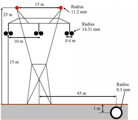
Consider in this case study an electrical system composed of a single horizontal circuit 400 kV overhead transmission line and a nearby buried metallic pipeline; the geometric parameters of the electrical system are presented in Figure 5. The three-phase AC system operates under balanced conditions, with each phase carrying a current of 2000 A at a nominal frequency of 50 Hz. The surrounding earth is considered homogeneous, characterized by a resistivity of 100 Ω·m. The alternating current (AC) resistance values for the conductors are specified as follows: 0.1586 Ω/km for the phase conductor, 0.1489 Ω/km for the earth (ground) wire, and 0.5 Ω/km for the metallic pipeline, the pipeline runs parallel to the electrical power line with an estimated influence length of 10 km; its coating is made by polyethylene (PE) material with an efficiency of 80%. The main electrical characteristics of the buried metallic pipeline are presented in Table 3 below:
Table 3. Characteristics of the electrical data of the pipeline
|
Parameter |
Value |
|
Resistivity of the soil (Ω.m) |
100 |
|
Resistivity of pipeline steel (Ω.m) |
1.7 × 10⁻⁷ |
|
Resistivity of pipeline coating (Ω.m) |
0.25 × 10⁷ |
|
Relative permeability of pipeline steel |
300 |
|
Relative permittivity of pipeline coating |
5 |
|
Thickness of the coating (m) |
0.005 |
Figure 5. EHV horizontal geometric configuration overhead power line (400 kV)
In the initial stage, the variation in the electromotive force along the underground metallic pipeline, resulting from inductive coupling, is analyzed as a function of its horizontal position relative to the power line corridor, as illustrated in Figure 6. The results reveal that the voltage reaches its minimum when the pipeline is positioned directly beneath the central phase conductor of the transmission line; then it increases progressively to reach a maximum value for a separation distance in the immediate vicinity of the lateral phase conductor. From this point; the induced voltage decreases rapidly with the increase of the lateral position of the pipeline from the power line center. It can be added that the increase of the soil resistivity allows to slightly reducing the induced voltage on the pipeline; the values of the induced voltage at the selected location of the pipeline for different values of soil resistivity are higher than the limit value recommended by the EN 50443 and CIGRE standards which is (50 V).
Figure 6. Variation of the induced voltage according to the position of the buried pipeline in the power line right-of-way
Figure 7. Distribution of induced voltage along the buried steel pipeline
Figure 7 illustrates the distribution pattern of the axial electromagnetic potential along the underground pipeline subjected to magnetic interference between its two terminals. It is evident that the peak potential values occur near both extremities, whereas the central section along the pipeline exhibits an almost negligible voltage level. Moreover, based on the variation over the pipeline’s length, it can be inferred that the geometric center of the pipeline relative to the ground acts as a point of symmetry.
Figure 8 demonstrates the influence of soil resistivity variations on the voltage induced in the metallic pipeline. It can be observed that changes in resistivity have a minimal impact, with higher resistivity values causing only a marginal reduction in the induced voltage.
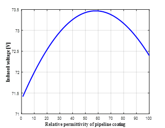
Figure 9 depicts how the induced voltage along the metallic pipeline varies with changes in the relative permittivity of the coating material. As shown, the AC induced voltage increases progressively, reaching a peak at a critical permittivity value, beyond which it declines sharply, eventually stabilizing at a significantly lower level as the permittivity continues to rise.
Figure 8. Influence of soil resistivity on the AC induced voltage in the buried pipeline
Figure 9. Effect of relative permeability of pipeline coating on AC induced voltage
Figure 10 illustrates how changes in the electrical resistance of the protective coating affect the magnitude of the voltage generated on the buried pipeline. The results indicate that as the coating resistivity rises, the induced voltage also increases progressively. However, beyond a specific resistivity threshold, the voltage stabilizes and exhibits only minor fluctuations, approaching a steady-state value.
Figure 11 examines the influence of the applied protective coating thickness of the on the AC induced voltage in the steel pipeline. The analysis shows that an increase in the coating thickness results in a quasi-linear increase in the induced voltage, with a significant initial phase followed by a deceleration. However, as soon as the thickness exceeds a certain threshold, the induced voltage value stabilizes around an approximately constant value.
Figure 12 presents the change in alternating current (AC) corrosion intensity along the buried pipeline in relation to the corresponding electromotive force. The findings reveal a linear increase in this intensity as the applied potential rises. Additionally, it is observed that the corrosive current magnitude is higher in low-resistivity soils compared to environments with higher resistivity. A very high value due to a low value of the soil resistivity can strongly produce the phenomenon of uniform corrosion of the steel constituting the buried pipeline.
Figure 10. Variation of induced voltage as a function of change in pipeline coating resistivity
Figure 11. Effect of pipeline insulation coating thickness on AC induced voltage
Figure 12. Relationship between AC induced voltage and corrosion current density in underground pipeline
Figure 13 depicts the variation in AC corrosion current density with respect to the size of a coating holiday. It is observed that as the diameter of the coating defect increases, the current density gradually decreases, indicating an inverse relationship between the two variables. Consequently, a buried pipeline with a small circular coating defect is more susceptible to uniform corrosion, as smaller defects tend to exhibit higher corrosion current densities compared to larger ones.
Figure 13. Effect of protective coating defect diameter on corrosion current density
Figure 14 illustrates how the metal’s degradation rate responds to changes in corrosion current density. This rate, representing how much material undergoes oxidation over time, is seen to rise proportionally with the applied AC current. As the electric current flowing through the corrosion site increases, both the rate of material loss and the extent of metal deterioration grow accordingly.
Figure 14. Corrosion rate profile as a function of corrosion current density
The second step is to design an optimal sacrificial anode cathodic protection system, which is a very important task because it takes into account different factors such as the optimal anode characteristics and the electrode current that ensure a good potential distribution over the pipeline to be protected.
To determine the most appropriate anode material for cathodic protection of a pipeline, a performance comparison is conducted between magnesium and zinc anodes, taking into account their electrochemical properties and expected lifespan—assuming both can meet the total required current. Let’s consider a buried metallic pipeline, with the same dimensions as previously described, located in soil with a resistivity of 30 Ω·m. A sacrificial cathodic protection system is designed using either magnesium or zinc anodes, intended to operate for 10 years. A protective current density of 0.5 mA/m² is applied over the entire pipeline surface, requiring the anodes to supply a total of 2 amperes while keeping the overall resistance below a defined critical value.
As shown in Figure 15, the magnesium anode meets this requirement using just 24 anodes, all while maintaining total resistance below the critical limit. In contrast, although the zinc system requires only 20 anodes to generate the same current, their combined resistance surpasses the allowable threshold. Further calculations indicate that at least 44 zinc anodes would be needed to satisfy the current demand without exceeding the resistance limit—significantly more than what is required for magnesium. Hence, magnesium is the preferred anode material due to its greater efficiency and ability to meet both current and resistance criteria effectively.
It is obvious that optimizing sacrificial anode cathodic protection requires a mathematical formulation with detailed equations using an objective function, design variables, and constraints. This resulting problem can be solved using an optimization algorithm.
Figure 15. Comparison of the efficiency of sacrificial anodes between magnesium and zinc metals
In order to effectively identify the best performing algorithm for solving the given optimization problem with a robust solution, a comparative performance analysis was conducted using several optimization methods widely adopted in the literature under identical conditions, in terms of solution quality, convergence speed, and execution time. These include the Grey Wolf Optimizer (GWO), Particle Swarm Optimization (PSO), Grasshopper Optimization Algorithm (GOA), and TLBO, as illustrated in Figure 16 [85].
Table 4 provides a summary of the parameter settings and the optimal objective function values obtained for each of the proposed optimization algorithms.
The performance comparison of the algorithms reveals that the TLBO method stands out for its rapid convergence to the optimal solution, delivering the lowest value when compared to the other approaches. This indicates that the TLBO is highly effective, offering superior efficiency and making it a strong contender for tackling the problem at hand.
Table 4. Setting parameters and optimal objective function values for the different proposed algorithms
|
Optimization Algorithms |
Setting Parameters |
Objective Function Value |
|
GWO |
Wolves number N = 20 Num_iter = 100 |
1.8e-03 |
|
PSO |
Swarm size N = 20, Learning factor c1 = 2, c2 = 2, Inertia weight w = 0.9, Num_iter =100 |
4.5e-04 |
|
GOA |
Search agents N = 20, cmax=1, cmin = 0.00001, Num_iter = 100 |
1.1e-04 |
|
TLBO |
Population size N = 20 Number iteration = 100 |
1.18e-05 |
Figure 16. Variation of the objective function values over the iterations of different proposed optimization algorithms
Figure 17 depicts the evolution of the objective function (OF) cited in Eq. (35) as a function of the number of iterations, using the TLBO optimization algorithm; it clearly presents the process of careful and continuous search for the optimal solution of the problem in the space of admissible objectives; by evaluating the objective function attributed to the minimization optimization process of the TLBO algorithm.
The optimization results of the objective function minimization for different obtained values relative to the search parameters of the objective function are presented in Figures 18-22; where it is clear that this algorithm converges quickly with better accuracy towards the optimal values of the considered variables after a limited number of iterations.
Figure 17. Variation of the objective function with the number of iterations of TLBO algorithm for the two poses of the anode
Figure 18. Variation of optimal soil resistivity values with the number of iterations
Figure 19. Variation of optimal values of anode dimensions with the number of iterations
The performance of cathodic protection systems is highly influenced by soil resistivity, which controls the density of the diffused current, the higher the current density, the more effective the protection, as well as the characteristics and location of the magnesium anodes. The parameters to be optimized include the soil resistivity, the anode size and weight, the electrochemical efficiency of the anode, the anode efficiency factor and the maximum life of each anode.
The various optimized parameters will be inserted directly into the cathodic protection design strategy by a magnesium-based sacrificial anode system.
The results from the application of the TLBO optimization algorithm regarding the estimation of the optimal parameters to be integrated into the calculation and dimensioning of the active protection system of the buried pipeline steel by the sacrificial anode method in order to improve the efficiency of the cathodic protection process are presented in Table 5.
Figure 20. Variation of optimal values of anode weight and electrochemical efficiency with the number of iterations
Figure 21. Variation of optimal values of anode efficiency factor and service life time with the number of iterations
Figure 22. Variation of optimal values of horizontal anode burial depth in ground with the number of iterations
Figure 23 describes the total protective current of the subterranean pipeline as a function of soil resistivity and coating degradation rate. The required protective current density is strongly related to soil resistivity; a pipeline installed in low-resistivity soil requires a higher protective current. Therefore, as soil resistivity increases, the required protective current decreases sharply. On the other hand, as coating effectiveness decreases due to coating degradation, the required protective current increases, and decreases strongly as coating effectiveness and quality increase.
Table 5. Optimal results of the variables resulting from the application of the TLBO algorithm
|
Characteristics of Soil and Magnesium Anodes |
Anode Arranged Vertically |
Anode Arranged Horizontally |
|
Resistivity of the soil (Ω.m) |
33 |
41 |
|
Utilization factor |
0.78 |
0.88 |
|
Anode weight requirement (kg) |
9 |
10.8 |
|
Anode current capacity (A.hr/kg) |
1000 |
1120 |
|
Anode lifetime (Year) |
20 |
24 |
|
Anode length (m) |
0.7 |
1.1 |
|
Anode diameter (m) |
0.22 |
0.32 |
|
Anode burial depth (m) |
/ |
0.96 |
Figure 23. Total protection current required as a function of soil resistivity
Figure 24. Calculation of total net weight and number of individual protective anodes
The overall anodic mass of the used material and the number of anodes required to maintain cathodic protection of the pipeline during its lifetime as a function of the total protection current are depicted in Figure 24. It can be clearly indicating the existence of a linear relationship between these two parameters and the total protection current; they increase proportionally with the current requirement for complete protection.
The calculation of the resistance of anode arranged in vertical and horizontal position as a function of soil resistivity is shown in Figure 25. In a soil assumed to be homogeneous, the resistance of an anodic material increases linearly as the soil resistivity increases; the soil which has a high resistivity does not allow having a relatively low resistance.
Figure 25. Variation of anode resistance in vertical and horizontal laying arrangement as a function of soil resistivity
The evaluation of the output current of each anode arranged in vertical or horizontal position compared t to the current requirement of each anode necessary to keep the sacrificial anode cathodic protection throughout the design period, depending on the soil resistivity is illustrated in Figure 26. As shown in this figure. The selected values of soil resistivity to meet the requirement of the specific design of the cathodic protection system must not exceed a critical value, so that the current generated by each localized anode must be slightly higher than the current required for each anode and necessary to protect the pipeline during its lifetime.
Figure 26. Comparison of output current and anode pipeline protection requirement current
The values optimized by the algorithm have proven to be able to meet the required conditions. From the curve shown in this figure, it is clearly seen that the amount of current that the anode can generate decreases sharply as the soil resistivity increases, while, the intensity of the galvanic protection current of each anode depends on the nominal electrochemical capacity of the anode; the number of hours in a year and its individual weight.
The important results of the analysis carried out for the optimal electrical design of the cathodic protection installation by the technological choice retained of the sacrificial anode arranged in vertical and horizontal position are summarized in Table 6.
Table 6. Results of the optimized analysis for the design of sacrificial anode cathodic protection
|
Basic Calculation Data for CP System |
Anode Arranged Vertically |
Anode Arranged Horizontally |
|
Pipeline metal current density (m.A/m2) |
25.47 |
24.26 |
|
Total protective current required (A) |
96.03 |
91.46 |
|
Total anode weight (kg) |
21569 |
19103 |
|
Number of anodes |
2397 |
1776 |
|
Protective current requirements for each anode (m.A) |
0.0401 |
0.0515 |
|
Electrolyte resistance (Ω) |
16.63 |
12.89 |
|
Current produced by the anode (m.A) |
0.0417 |
0.0539 |
The comparison of results in terms of pipeline protection current requirement between the anode output current and the anode current capacity is perfectly respected. This criterion must be achieved at any point in the pipeline after the system is commissioned and whatever the operating conditions.
To assess the robustness and validity of the proposed approach, the results have been benchmarked against a case study detailed in reference [86]. This reference scenario involves a buried steel pipeline with a length of 100 meters and a diameter of 0.3 meters, subjected to varying soil resistivity conditions. The pipeline is protected using magnesium anodes with dimensions, length = 48 cm, and diameter = 12 cm, while a protective current density of 10 mA/m² is maintained. A summary of the calculated results for this configuration is provided in Table 7.
Table 7. A comparison of the results from the applied calculation program with the reference [86]
|
Soil Resistivity (Ω.cm) |
Adopted Method |
Reference [86] |
||
|
Total Number of Anodes |
Output Current Per Anode (A) |
Total Number of Anodes |
Output Current Per Anode (A) |
|
|
600 |
27 |
0.31 |
29 |
0.35 |
|
1000 |
45 |
0.21 |
48 |
0.21 |
|
5000 |
225 |
0.050 |
240 |
0.042 |
From the comparison of the results presented in the table, it is clear that there is a high degree of agreement, with a small error margin that remains within the acceptable tolerance and can be ignored.
Adverse effects between EHV power lines and metallic pipelines in a common service corridor are unavoidable due to AC inductive coupling. In this study, a rigorous quasi-static modeling using transmission line approach is adopted to evaluate the effects of AC electromagnetic interference and implementing mitigation measure to eliminate the undesirable effects by employing the meta-heuristic optimization algorithms. From the results, it is clear that the induced voltage appearing in the metal pipeline varied greatly depending on its position relative to the electricity pylon. In certain cases, the induced voltage surpasses the permissible limit specified by international standards (EN 50443) and thus causes the generation of a current density that leads to the phenomenon of corrosion of the pipeline metal by causing leaks, cracks and rupture of the pipeline and to harmful effects in the medium or long term on the structural stability and integrity of the hydrocarbon transport system. The corrosion behavior of the metal is characterized by the corrosion rate which is proportional to the current density; it can be expressed in terms of mass loss or reduction in thickness of the buried metallic pipeline.
Pipeline corrosion control is achieved by designing an appropriate cathodic protection system with sacrificial anode; the sizing procedure is based on a more reliable optimization process using the TLBO algorithm. The basic parameter is the soil resistivity which can have a major impact on the dimensions of the cathodic protection system where a low resistivity provides an effective corrosion protection system, in addition the characteristics and dimensions of the sacrificial anodes. The sizing is done on the basis of the total current required for the protection of the pipeline and the minimum number of anodes required for the protection. It has been found that this adopted strategy is capable of protecting the metallic pipeline from corrosion, by meeting the total current requirement for adequate protection. A properly installed sacrificial anode cathodic protection remains a more effective solution for the proper functioning of buried metallic pipelines. By comparing the adopted methodology with values from the literature, a satisfactory correlation is observed, validating its accuracy and reliability.
The authors would like to thank the head the and staff of Laboratory for Analysis and Control of Energy Systems and Electrical Networks (LACoSERE), University of Laghouat, Laghouat (03000), Algeria.
|
${{A}_{p}}$ |
Surface area of pipeline to be protected (m2) |
|
${{B}_{T}}$ |
Magnetic induction (μT) |
|
${{C}_{a}}$ |
Anode current capacity (A.hr/kg) |
|
$CE$ |
Efficiency coating of pipeline (%) |
|
${{D}_{a}}$ |
Equivalent diameter of anode (m) |
|
${{d}_{h}}$ |
Diameter of the circular holiday(m) |
|
$\text{Dif}{{\text{f}}_{\text{i}}}$ |
Difference between the teacher and the population average |
|
${{d}_{ij}}$ |
Distance between the power line conductor and the pipeline (m) |
|
$d_{ij}^{'}$ |
Distance between the image of the power line conductor and the pipeline (m) |
|
${{D}_{e}}$ |
Depth of earth penetration (m) |
|
${{D}_{p}}$ |
Diameter of buried metallic pipeline (m) |
|
${{E}_{a}}$ |
Voltage of the pipeline at rest (V) |
|
${{E}_{ind}}$ |
Induced electromotive force (V/m) |
|
${{E}_{prot}}$ |
Voltage protection of the pipeline (V) |
|
${{f}_{s}}$ |
Safety factor |
|
${{h}_{a}}$ |
Twice depth of anode (m) |
|
${{I}_{a}}$ |
Protection current required for each anode (mA) |
|
${{I}_{g}}$ |
Current generated by each anode (m.A) |
|
${{I}_{i}}$ |
Current flowing through the power line conductor (A) |
|
${{I}_{ind}}$ |
Induced current along the pipeline (A) |
|
${{I}_{t}}$ |
Total current requirement for cathodic protection (A) |
|
${{J}_{ac}}$ |
AC current density of corrosion (m.A/m2) |
|
${{J}_{p}}$ |
Design current density (m.A/m2) |
|
${{l}_{a}}$ |
Length of anode (m) |
|
${{L}_{p}}$ |
Parallelism length of the inductive coupling exposure (A) |
|
${{M}_{m}}$ |
Atomic weight (g) |
|
${{M}_{i}}$ |
Average of all students in the class |
|
${{R}_{a}}$ |
Resistance of anode (Ω) |
|
${{R}_{c}}$ |
Coating resistance (Ω) |
|
${{R}_{is}}$ |
Insulation resistance of the coating pipeline (Ω) |
|
${{R}_{ps}}$ |
Pipeline to electrolyte resistance (Ω) |
|
${{R}_{t}}$ |
Total propagation resistance (Ω) |
|
${{s}_{h}}$ |
Surface area of circular holiday (m2) |
|
${{S}_{prot}}$ |
Total external surface of pipeline to be protected (m2) |
|
${{t}_{c}}$ |
Corrosion time (sec) |
|
${{U}_{f}}$ |
Utilization factor of anode |
|
${{V}_{ind}}$ |
Induced voltage in pipeline (V) |
|
${{W}_{a}}$ |
Weight of one anode (kg) |
|
${{W}_{t}}$ |
Total weight of anodes to be installed (kg) |
|
${{X}_{j,i}}$ |
Best solution |
|
$X_{j,i}^{'}$ |
New best solution |
|
${{X}_{T,i}}$ |
Result of the best learner in subject |
|
$y$ |
Admittance per unit length of buried pipeline (S) |
|
$Y$ |
Design life time (Year) |
|
$z$ |
Impedance per unit length of buried pipeline (Ω) |
|
${{z}_{e}}$ |
Charge number |
|
${{Z}_{c}}$ |
Characteristic impedance of buried pipeline |
|
Greek symbols |
|
|
$\gamma $ |
Propagation constant of the buried pipeline |
|
${{\delta }_{c}}$ |
Thickness of coating (m) |
|
${{\varepsilon }_{0}}$ |
Permittivity of free space (8.85 × 10⁻¹² F/m) |
|
${{\varepsilon }_{r}}$ |
Coating’s relative permittivity |
|
${{\mu }_{0}}$ |
Permeability of free space (4π × 10-7 H/m) |
|
${{\mu }_{p}}$ |
Relative permeability of pipeline’s metal |
|
$\pi $ |
Greek letter, geometric constant approximately equal to 3.1416 |
|
${{\rho }_{c}}$ |
Resistivity of pipeline’s coating (Ω.m) |
|
${{\rho }_{f}}$ |
Resistivity of electrolyte (Ω.m) |
|
${{\rho }_{m}}$ |
Specific density of metal (kg/m3) |
|
${{\rho }_{s}}$ |
Soil resistivity (Ω. cm) |
|
$\varphi $ |
Magnetic flux (Wb) |
|
$\omega $ |
Angular power frequency (rad/sec) |
|
Subscripts |
|
|
AC |
Alternating Current |
|
AI |
Artificial Intelligence |
|
CEN |
Comité européen de normalisation (European Committee for Standardization) |
|
$Cu$ |
Chemical symbol of Copper element |
|
$CuSO4$ |
Chemical symbol of Copper sulfate |
|
DC |
Direct Current |
|
DIN |
Deutsches Institut für Normung (German Institute for Standardization) |
|
DNV |
DET NORSKE VERITAS |
|
${{e}^{-}}$ |
Electron symbol |
|
EHV |
Extra High Voltage |
|
EN |
European Norm |
|
EO |
Evolutionary Optimization |
|
$F$ |
Faraday's constant $\text{F}=96.485\text{ }\!\!~\!\!\text{ C}/\text{mol}$ |
|
$Fe$ |
Chemical symbol of Iron element |
|
$GOA$ |
Grasshopper Optimization Algorithm |
|
$GWO$ |
Grey Wolf Optimizer |
|
H2O |
Chemical symbol of water molecule |
|
j |
Imaginary nuer |
|
ISO |
International Organization for Standardization |
|
$\text{Mg}$ |
Chemical symbol of Magnesium element |
|
NACE |
National Association of Corrosion Engineers |
|
NF |
Norme Française |
|
$OF$ |
Objective Function |
|
$OH$ |
Chemical symbol of Hydroxide anion |
|
${{O}_{2}}$ |
Chemical symbol of oxygen molecule |
|
$PE$ |
Polyethylene material coating |
|
$PSO$ |
Particle Swarm Ooptimization |
|
${{r}_{i}}$ |
Random number |
|
${{T}_{F}}$ |
Teacher factor |
|
TLBO |
Teaching Learning Based Optimization |
|
TS |
Technical Specification |
|
$\text{Zn}$ |
Chemical symbol of zinc element |
[1] Panagiotis, S.I., Georgia, P. (2013). Transportation of energy resources in the Middle East and Central Asia. International Journal of Energy Economics and Policy, 3(4): 127-139.
[2] Mikail, E., Çora, H., Çora, A. (2020). Azerbaijan’s energy resources and BTC (Bakü Tbilisi Ceyhan is the name given to the pipeline project being built for crude oil transfer) project. Open Journal of Political Science, 10(2): 163-184. https://doi.org/10.4236/ojps.2020.102012
[3] Canadian Association of Petroleum Producers, Guide Capp. (2014). Influence of High Voltage DC Power Lines on Metallic Pipelines, EA-2014-0207.
[4] Al-Badi, A.H., Al-Rizzo H.M. (2005). Simulation of electromagnetic coupling on pipelines close to overhead transmission lines: A parametric study. Journal of Communications Software and Systems, 1(2): 116-125.
[5] CIGRE. (1995). Guide on the Influence of High Voltage AC Power Systems on Metallic Pipelines. Working Group 36.02, Technical Brochure no. 095, Paris, France.
[6] NACE International Standard. (2014). Mitigation of Alternating Current and Lightning Effects on Metallic Structures and Corrosion Control Systems. NACE International, SP0177, Houston, TX, USA.
[7] CIGRE/CIRED. (2006). AC Corrosion on Metallic Pipelines Due to Interference from AC Power Lines Phenomenon, Modeling and Countermeasures. Joint Working group, C4.2.02, ELECTRA, no. 225: 63-69.
[8] Kadhim, M.G., Ali, M.T.A. (2017). A critical review on corrosion and its prevention in the oil field equipment. Journal of Petroleum Research and Studies, 7(2): 162-189.
[9] Chen, Z., Koleva, D., Van-Breugel, K. (2017). A review on stray current-induced steel corrosion in infrastructure. Corrosion Reviews, 35(6): 397-423. https://doi.org/10.1515/corrrev-2017-0009
[10] NACE International Standard. (2010). AC Corrosion State of the Art: Corrosion Rate, Mechanism, and Mitigation Requirements, NACE, TG 327, Report 35110, Houston, USA.
[11] Chen, X., Li, X.G., Du, C.W., Cheng, Y.F. (2009). Effect of cathodic protection on corrosion of pipeline steel under disbonded coating. Corrosion Science, 51(9): 2242-2245. https://doi.org/10.1016/j.corsci.2009.05.027
[12] Hussein-Farh, H.M., El Amine Ben Seghier, M., Zayed, T. (2023). Comprehensive review of corrosion protection and control techniques for metallic pipelines. Engineering Failure Analysis, 143: 106885. https://doi.org/10.1016/j.engfailanal.2022.106885
[13] Hussein Farh, H.M., Ben Seghier, M.E.A., Taiwo, R., Zayed, T. (2023). Analysis and ranking of corrosion causes for water pipelines: A critical review. NPJ Clean Water, 6(1): 65. https://doi.org/10.1038/s41545-023-00275-5
[14] Byrne, A., Holmes, N., Norton, B. (2016). State of the art review of cathodic protection for reinforced concrete structures. Magazine of Concrete Research, 68(13): 664-677. https://doi.org/10.1680/jmacr.15.00083
[15] Angst, U.M. (2019). A critical review of the science and engineering of cathodic protection of steel in soil and concrete. Corrosion, 75(12): 1420-1433. https://doi.org/10.5006/3355
[16] Thompson, A.A., Wood, J.L., Palombo, E.A., Green, W.K., Wade, S.A. (2022). From laboratory tests to field trials: A review of cathodic protection and microbially influenced corrosion. Biofouling, 38(3): 298-320. https://doi.org/10.1080/08927014.2022.2058395
[17] Guo, Z., Xiao, Z., Chen, H., Zhou, X., Wang, P., Luo, J., Gao, Y., Shang, H. (2024). Review of cathodic protection technology for steel rebars in concrete structures in marine environments. Applied Sciences, 14(19): 9062. https://doi.org/10.3390/app14199062
[18] BS EN 12954. (2019). General principles of cathodic protection of buried or immersed onshore metallic structures. British Standards Institution (BSI).
[19] DNV. (2010). Cathodic Protection Design, Recommended Practice DNV-RP-B401.
[20] Liang, H., Wu, Y., Han, B., Lin, N., Wang, J., Zhang, Z., Guo, Y. (2025). Corrosion of buried pipelines by stray current in electrified railways: Mechanism, influencing factors, and protection. Applied Sciences, 15(1): 264. https://doi.org/10.3390/app15010264
[21] Diedericks, D.E., van Schoor, G., Ranft, E.O. (2019). Cathodic protection system design framework. In 2019 Southern African Universities Power Engineering Conference/Robotics and Mechatronics/Pattern Recognition Association of South Africa (SAUPEC/RobMech/PRASA), Bloemfontein, South Africa, pp. 530-537. https://doi.org/10.1109/RoboMech.2019.8704760
[22] Khazreai, M.A. (2006). Short History of Cathodic protection for fixed offshore structure. The Journal of Corrosion Science and Engineering, 9: 47.
[23] Hammajam, A.A., Ibrahim, M.A., Adam, M.K. (2022). Design, analysis and construction of an impressed current electric device for cathodic protection. Arid Zone Journal of Engineering, Technology and Environment, 18(2): 183-196.
[24] Muhaned, M.A. (2019). Impressed current cathodic protection for oil well casing and associated flow lines. African Journal of Electrical and Electronics Research, 1(1): 1-8.
[25] Moe, M.S.C., Chong, C. (2013). Application of cathodic protection for controlling macrocell corrosion in chloride contaminated RC structures, Construction and Building Materials, 45: 199-207. https://doi.org/10.1016/j.conbuildmat.2013.04.010
[26] Jasim, D.M., Razzaq Hussein, E.A., Al-Libawy, H. (2023). Cathodic protection systems: Approaches and open challenges. Nexo Revista Científica, 36(6): 956-967. https://doi.org/10.5377/nexo.v36i06.17451
[27] Rao, R.V., Savsani, V.J., Vakharia, D.P. (2011). Teaching–learning-based optimization: A novel method for constrained mechanical design optimization problems. Computer-Aided Design, 43(3): 303-315. https://doi.org/10.1016/j.cad.2010.12.015
[28] Gherbia, A., Djekidel, R., Bessedik, S.A., Mahi, D. (2023). AC Corrosion phenomenon and mitigation in buried pipeline due to very high voltage overhead transmission line effect. Facta Universitatis Series: Electronics and Energetics, 36(3): 427-447. https://doi.org/10.2298/FUEE2303427G
[29] Djekidel, R., Mahi, D. (2014). Calculation and analysis of inductive coupling effects for HV transmission lines on aerial pipelines. Przegląd Elektrotechniczny, 90(9): 151-156.
[30] Lee, H.G., Ha, T.H., Ha, Y.C., Bae, J.H., Kim, D.K. (2004). Analysis of voltages induced by distribution lines on gas pipelines. In 2004 International Conference on Power System Technology, 2004. PowerCon 2004, Singapore, pp. 598-601. https://doi.org/10.1109/ICPST.2004.1460064
[31] Adedeji, K.B., Abe, B.T., Hamam, Y., Abu-Mahfouz, A.M., Shabangu, T.H., Jimoh, A.A. (2017). Pipeline grounding condition: A control of pipe-to-soil potential for AC interference induced corrosion reduction. In the 25th Southern African Universities Power Engineering Conference, Stellenbosch, South Africa, pp. 577-582.
[32] Al-Gabalawy, M.A., Mostafa, M.A., Abdel-Salam, H., Shimaa, A.H. (2020). Modeling of the KOH-Polarization cells for mitigating the induced AC voltage in the metallic pipelines. Heliyon, 6(3): e03417. https://doi.org/10.1016/j.heliyon.2020.e03417
[33] Bouallag, K., Djekidel, R. Bessedik, S.A. (2021). Optimization of induced voltage on buried pipeline from HV power lines using grasshopper algorithm (GOA). Diagnostyka, 22(2): 105-115. https://doi.org/10.29354/diag/138719
[34] Bortels, L., Parlongue, J., Fieltsch, W., Segall, S. (2010). Manage pipeline integrity by predicting and mitigating HVAC interference. In Proceedings of the NACE-International Corrosion Conference Series; Nace International: San Antonio, TX, USA, pp. 1-15. https://doi.org/10.5006/C2010-10114
[35] Bosch, R.W., Bogaerts, W.F. (1998). A theoretical study of AC-induced corrosion considering diffusion phenomena. Corrosion Science, 40(2-3): 323-336. https://doi.org/10.1016/S0010-938X(97)00139-X
[36] Heim, G., Heim, T., Heinzen, H., Schwenk, W. (1993). Investigation of corrosion of cathodically protected steel subjected to alternating currents. 3R International, 32(5): 246-249.
[37] Zhang, R., Vairavanathan, P.R., Lalvani, S.B. (2008). Perturbation method analysis of AC-induced corrosion. Corrosion Science, 50(6): 1664-1671. https://doi.org/10.1016/j.corsci.2008.02.018
[38] ISO 18086. (2015). Corrosion of metals and alloys, Determination of AC corrosion, Protection criteria. International Organization for Standardization, Geneva, Switzerland.
[39] Choi, B.Y., Lee, S.G., Kim, J.K., Oh, J.S. (2016). Cathodic protection of onshore buried pipelines considering economic feasibility and maintenance. Journal of Advanced Research in Ocean Engineering, 2(4): 158-168. https://doi.org/10.5574/JAROE.2016.2.4.158
[40] Guo, Y.B., Liu, C., Wang, D.G., Liu, S.H. (2015). Effects of alternating current interference on corrosion of X60 pipeline steel. Petroleum Science, 12(2): 316-324. https://doi.org/10.1007/s12182-015-0022-0
[41] Ameh, E.S., Ikpeseni, S.C., Lawal, L.S. (2018). A review of field corrosion control and monitoring techniques of the upstream oil and gas pipelines. Nigerian Journal of Technological Development, 14(2): 67-73. https://doi.org/10.4314/njtd.v14i2.5
[42] Simon, P.D. (2010). Overview of HVAC transmission line interference issues on buried pipelines. In NACE Northern Area Western Conference, Canada, pp. 1-21.
[43] Wakelin, R.G., Gummow, R.A., Segall, S.M. (1998). AC corrosion–case histories, test procedures, and mitigation. In Corrosion 1998, NACE International, paper no. 565, Houston, USA, pp. 1-14. https://doi.org/10.5006/C1998-98565
[44] Gummow, R.A., Wakelin, R.G, Segall, S.M. (1998). AC corrosion-A new challenge to pipeline integrity. In Corrosion 1998, NACE International, paper no.566, San Diego, USA, pp. 1-18. https://doi.org/10.5006/C1998-98566
[45] UKOPA. (2019). AC Corrosion Guidelines. Good Practice Guide, UKOPA/GPG/027, United Kingdom.
[46] Abdullah, N. (2021). HVAC interference assessment on a buried gas pipeline. Conference Series: Earth and Environmental Science, 704(1): 012009. https://doi.org/10.1088/1755-1315/704/1/012009
[47] Hosokawa, Y., Koriyama, F., Nakamura, Y. (2002). New CP criteria for elimination of the risks of AC corrosion and overprotection on cathodically protected pipelines. Corrosion, NACE International, no. 02111, Denver, USA.
[48] Freiman, L.I., Kuznetsova, E.G. (2001). Model investigation of the peculiarities of the corrosion and cathodic protection of steel in the insulation defects on underground steel pipelines. Protection of Metals, 37: 484-490. https://doi.org/10.1023/A:1012378500386
[49] Kouloumbi, N., Batis, G., Kioupis, N., Kioupis, N., Asteridis, P. (2002). Study of the effect of AC-interference on the cathodic protection of a gas pipeline. Anti-Corrosion Methods and Materials, 49(5): 335-345. https://doi.org/10.1108/00035590210440728
[50] Union Gas Ltd. (2016). AC Interference Study. NPS12-15136-20, Leamington Expansion, Phase II, Ontario, Canada.
[51] DIN 50929-3. (1985). Corrosion of metals–Probability of corrosion of metallic materials when subject to corrosion from the outside – buried and underwater pipelines and structural components. German Institute for Standardization, Berlin, Germany.
[52] CEN/TS 15280. (2006). Evaluation of ac corrosion likelihood of buried pipelines–application to cathodically protected pipelines. Technical Specification, CEN - European Committee for Standardization, Germany.
[53] Adedeji, K.B., Ponnle, A.A., Abe, B.T., Jimoh, A.A., Abu-Mahfouz, A.M., Hamam, Y. (2018). AC induced corrosion assessment of buried Pipelines near HVTLs: A case study of South Africa. Progress in Electromagnetics Research B, 81: 45-61. https://doi.org/10.2528/PIERB18040503
[54] Wong, L.L., Martin, S.I., Rebak, R.B. (2006). Methods to calculate corrosion rates for alloy 22 from Polarization resistance experiments. In Proceedings of the ASME Pressure Vessels and Piping Division Conference, Vancouver, Canada, pp. 571-580. https://doi.org/10.1115/PVP2006-ICPVT-11-93421
[55] Hossam-Eldin, A.A., Elgamal, M.E., Aly, A.A. (2023). Detailed study of electrical interference coupling between AC OHTL and buried metallic pipelines. In 24th International Middle East Power System Conference, Mansoura, Egypt, pp. 1-8. https://doi.org/10.1109/MEPCON58725.2023.10462360
[56] Malaret, F., Yang, X.S. (2022). Exact calculation of corrosion rates by the weight-loss method. Experimental Results, 3: e13. https://doi.org/10.1017/exp.2022.5
[57] Wang, H., Yu, C., Wang, S., Gao, J. (2015). Electrochemical corrosion behavior and prediction of corrosion rate for low alloy steel after tempering treatment. International Journal of Electrochemical Science, 10(2): 1169-1185. https://doi.org/10.1016/S1452-3981(23)05063-0
[58] Sun, F., Li, X., Zhang F., Cheng, X., Zhou, C., Wu, N., Yin, Y., Zhao, J. (2013). Corrosion mechanism of corrosion-resistant steel developed for bottom plate of cargo oil tanks. Acta Metallurgica Sinica, 26: 257-264. https://doi.org/10.1007/s40195-012-0231-0
[59] Choi, O.C., Park, Y.S., Ryu, H.Y. (2008). Corrosion evaluation of epoxy-coated bars by electrochemical impedance spectroscopy. International Journal of Concrete Structures and Materials, 2(2): 99-105. https://doi.org/10.4334/ijcsm.2008.2.2.099
[60] Ezekiel Enterprises-LLC. (2015). Introduction to Electrical Design for Cathodic Protection System. Ezekiel Enterprises, Course EE410.
[61] Ameh, E.S., Ikpeseni, S.C. (2017). Pipelines cathodic protection design methodologies for impressed current and sacrificial anode systems. Nigerian Journal of Technology, 36(4): 1072-1077. https://doi.org/10.4314/njt.v36i4.12
[62] Deepak, S.M., Rafael, E.R. (2006). Designing cathodic protection system under the influence of high voltage AC interference. In the NACE International Annual Conference, pp. 1-9. https://doi.org/10.5006/C2006-06162
[63] Abomadina, M.M. (2021). Design of cathodic protection for underground crude-oil pipeline by sacrificial anodes systems. Sirte University Scientific Journal, 11(1): 67-74.
[64] Abdulaaima, D.A., Omara, W.I., Kadhim, R.J., Ibrahim, B.K., Abdulkareem, M.M., Shehadha, M.A. (2022). Modelling & simulation for West Qurna (Tuba-1) cathodic protection design by using MATLAB Simulink. Journal of Petroleum Research and Studies, 12(1): 317-331. https://doi.org/10.52716/jprs.v12i1.605
[65] Salah, M.E., Mohamed, A.G., Farag I.M.H., Hussein, S.B. (2012). Evaluation of sacrificial cathodic protection on a large PCCP pipeline system. In 30th International Conference on Corrosion Mitigation and Surface Protection Technologies, Hurghada, Egypt, pp. 78- 84.
[66] Meillier, A. (2000). A Review of Galvanic Anode Cathodic Protection Design Procedure. Corrosion Control Services Limited, Telford, UK.
[67] El-Ashraf, A.I., Ahmed, A.M., Hossam-Eldin, A. (2013). Design of a cathodic protection system to prevent corrosion of metallic structures using hybrid renewable energy sources. Engineering Research Journal, 36(2): 109-1173. https://doi.org/10.21608/erjm.2013.67057
[68] Lilly, M.T., Ihekwoaba, S.C., Ogaji, S.O.T., Probert, S.D. (2007). Prolonging the lives of buried crude-oil and natural-gas pipelines by cathodic protection. Applied Energy, 84(9): 958-970. https://doi.org/10.1016/j.apenergy.2007.03.002
[69] Kalovelonis, D.T., Gortsas, T.V., Tsinopoulos, S.V., Polyzos, D. (2025). A novel design methodology for sacrificial anode cathodic protection systems using numerical modeling: A case study of offshore wind turbine monopile foundations. Ocean Engineering, 318: 12016. https://doi.org/10.1016/j.oceaneng.2024.120169
[70] Al-Habobi, N.A., Abed, S.F. (2013). Simulation of cathodic protection system using Matlab. Iraqi Journal of Chemical and Petroleum Engineering, 14(1): 25-37. https://doi.org/10.31699/IJCPE.2013.1.3
[71] Sari, N.H., Suteja., Lelio, R. (2021). Corrosion protection by sacrificial anode method on underground solar pipe installation: A case study in the Lombok Gas Engine Combine Cycle Power plant (Peaker) 130-150 MW. Journal of Energy, Mechanical, Material, and Manufacturing Engineering, 6(2): 97-102. https://doi.org/10.22219/jemmme.v6i2.11519
[72] Oghli, H.M., Akhbari, M., Kalaki, A., Eskandarzad, M. (2020). Design and analysis of the cathodic protection system of oil and gas pipelines, using distributed equivalent circuit model. Journal of Natural Gas Science and Engineering, 84: 103701. https://doi.org/10.1016/j.jngse.2020.103701
[73] Jawad, M.N., Mahdiraji, G.A., Hajibeigy, M.T. (2020). Performance improvement of sacrificial anode cathodic protection system for above ground storage tank. SN Applied Sciences, 2: 1979. https://doi.org/10.1007/s42452-020-03823-7
[74] Yu, K., Wang, X., Wang, Z. (2016). An improved teaching-learning-based optimization algorithm for numerical and engineering optimization problems. Journal of Intelligent Manufacturing, 27: 831-843. https://doi.org/10.1007/s10845-014-0918-3
[75] Bouchekara, H.R.E.H., Abido, M.A., Boucherma, M. (2014). Optimal power flow using teaching learning based optimization. Electric Power Systems Research, 114: 49-59. https://doi.org/10.1016/j.epsr.2014.03.032
[76] Sarzaeim, P., Bozorg-Haddad, O., Chu, X. (2018). Teaching-Learning-Based Optimization (TLBO) Algorithm. In Advanced Optimization by Nature-Inspired Algorithms. Studies in Computational Intelligence, pp. 51-58. https://doi.org/10.1007/978-981-10-5221-7_6
[77] Puralachetty, M.M., Pamula, V.K., Gondela, L.M., Akula, V.N.B. (2016). Teaching-learning-based optimization with two-stage initialization. In Proceedings of the IEEE Students' International Conference on Electrical, Electronics and Computer Science. Bhopal, pp. 1-5. https://doi.org/10.1109/SCEECS.2016.7509340
[78] Venkata- Rao, R., Vivek, P. (2013). An improved teaching-learning-based optimization algorithm for solving unconstrained optimization problems. Scientia Iranica, 20(3): 710-720. https://doi.org/10.1016/j.scient.2012.12.005
[79] Bozorg-Haddad, O., Sarzaeim, P., Loáiciga, H.A. (2021). Developing a novel parameter-free optimization framework for flood routing. Scientific Reports, 11(1): 16183. https://doi.org/10.1038/s41598-021-95721-0
[80] Djekidel, R., Mohamed, L., Ghoneim-Sherif, S.M., Mahi, D. (2022). Combined effects of electrostatic and electromagnetic interferences of High Voltage power lines on aerial metallic pipeline. Facta Universitatis Series: Electronics and Energetics, 35(3): 349-377. https://doi.org/10.2298/FUEE2203349R
[81] Rao, R.V., Patel, V. (2012). An elitist teaching-learning-based optimization algorithm for solving complex constrained optimization problems. International Journal of Industrial Engineering Computations, 3(4): 535-560. https://doi.org/10.5267/j.ijiec.2012.03.007
[82] He, X., Huang, J., Rao, Y., Gao, L. (2016). Chaotic teaching-learning-based optimization with Lévy flight for global numerical optimization. Computational Intelligence and Neuroscience, 2016(1): 8341275. https://doi.org/10.1155/2016/8341275
[83] Sleesongsom, S., Bureerat, S. (2017). Four-bar linkage path generation through self-adaptive population size teaching-learning based optimization. Knowledge-Based Systems, 135: 180-191. https://doi.org/10.1016/j.knosys.2017.08.012
[84] Meriouma, T., Bessedik, S.A., Djekidel, R. (2021). Modelling of electric and magnetic field induction under overhead power line using improved simulation techniques. European Journal of Electrical Engineering, 23(4): 289-300. https://doi.org/10.18280/ejee.230402
[85] Hussien, A.G., Hassanien, A.E., Houssein, E.H. (2017). Swarming behaviour of salps algorithm for predicting chemical compound activities. In 8th International Conference on Intelligent Computing and Information Systems (ICICIS), Cairo, Egypt, pp. 315-320. https://doi.org/10.1109/INTELCIS.2017.8260072
[86] Abdulamer, D.N. (2013). Effect of soil resistivity on the design of sacrificial anode cathodic protection system. Journal of Petroleum Research and Studies, 4(3): 142-158. https://doi.org/10.52716/jprs.v4i3.121