Ahmed Hameed Reja*![]() | Mazin Abdulaali Hamzah
| Mazin Abdulaali Hamzah![]()
© 2025 The authors. This article is published by IIETA and is licensed under the CC BY 4.0 license (http://creativecommons.org/licenses/by/4.0/).
OPEN ACCESS
With the development of modern communications systems, and the increased need for effective air defense and surveillance systems to improve tracking, command and guidance systems for unmanned aerial vehicles (UAVs), the need to improve and develop aerial monitoring devices to assist in the process of detecting moving targets with high accuracy and efficiency has increased. Since air surveillance systems and radars require human monitoring, they remain subject to error and inaccuracy. As a result of relying on this human factor, aircraft surveillance and navigation systems cannot be completely relied on human effort as their performance varies depending on the efficiency of the operators. In this study, an air surveillance system for navigation and radar devices was proposed that works with smart technologies to detect moving targets and control air navigation. Artificial neural networks (ANNs) and conventional neural network (CNN) technologies are used to automatically identify and classify moving targets in the navigation system. The data of the moving object through reflected signals and radar images is fed into the training module of the Artificial Intelligence (AI) system, which is an algorithm to plot and track the path of the moving object based on the reflected radar signals. The accuracy of the results of the AI system depends on the accuracy of the radar signals reflected from the moving object to represent the data output to the ANN. Simulation results showed that intelligent navigation can accurately identify various targets and chart their path with high efficiency. Through the results obtained by implementing AI algorithms, it is possible to control air navigation by following and detecting moving targets. The simulation results of the CNNs technology showed a high efficiency in controlling and tracking targets, reaching 97%, with robust implementation for moving target detection and tracking simulation using efficient deep learning FRCNN algorithm updated by applying MATLAB and tested on a set of data for images of various moving UAVs. Also, the results of several tests showed the success of the applied algorithm design in identifying and detecting moving targets at small error rate of 0.01 with a good training speed for the tested data set of 12 seconds.
unmanned aerial vehicles, navigation control, moving target, convolutional neural networks, object motion recognition
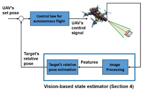
It is obvious thing for air navigation systems to be able to point out targets being tracked without the required for human involvement, while this is not every time the case. Air navigation and surveillance systems cannot be relied upon in these situations because the performance of operator vary frequently. To upgrade the performance and stability of the radar and navigation system, autonomous capabilities for moving target detection and identification are needed. In this study the reliance on human operators to follow and monitor aerial objects is reduced. By combining the cognitive engine, neural network, and air navigation and control system to be able to build a smart radar system instead of an experience human operator [1-4]. Radar networks and aerial surveillance have been intelligently added to the concept of artificial learning in the past decade. This system has the ability to preserve environment data much preferable than an individual radar component. Previous studies presented various techniques about air navigation, detection, tracking, identifying and controlling moving targets, but the real challenge emerged through the scenario of attempts to identify shapes of moving objects, which are often present in air monitoring systems, which include problems of environmental conditions, altitude, and speed [5, 6]. Studies and investigations in this field were somewhat weak, as it became necessary to build intelligent navigation and control systems that can assist the human side and enhance the capabilities of pilots, control elements, operators, and command personnel in order to ensure appropriate protection of aircraft and the airspace. The need for intelligent tracking systems is increasing, especially in the leave of appropriate sensors, radio receivers and cameras, and systems that recognize warning at an equitable pace without burdening the entire surveillance system with false warnings. Artificial Intelligence (AI) technologies help reduce the difficulties faced by moving object detection systems, which improves the security aspect. This includes moving human surveillance aircraft, vehicles and low-flying aircraft as suitable targets. Furthermore, the mission of air surveillance and control is to verify the classification of moving targets through different transport settings, both ground and air. How the navigation and control system works is covered in more technical and practical detail than in this work. The framework of the developed neural network dedicated to classifying radar targets will also be studied. To obtain automated classification results for such simulations using an AI, based on radar detection of typical moving targets. Figure 1 shows a typical intelligent surveillance UAV system signal process for moving targets [6-10]. A summary of the work of air surveillance and control systems will be explained in general by clarifying their mechanism of operation. First, the UAV drone's radar sends an RF signal to determine the target's range, speed and direction as it is analyzed and processed. A vehicle, or other moving target may be detected within the radar range where it is identified. There are three different operating modes to which monitoring can be applied. Initial target detection will be through the use of a high-resolution Doppler device, with an inverse synthetic aperture radar. In the future, the neural network applies high-resolution images for analysis, and must be superior to operating modes on radar to obtain the preferable results. Once the search location is determined, changing the control and tracking parameters to accurately locate the target is critical. Secondly, improving the location of the target has an impact on the frequency of the returned signal to determine the extent of the target’s progress, as the monitoring system is committed to advancing between the transmitting and receiving modes of the returned signal, accompanied by a Doppler shift of the reflected signal. Next, high-resolution profiles are used for the viewing frame to provide a high 2-D image. Accuracy of the object or target is a point of interest [7-12].
Figure 1. Schematic diagram of intelligent surveillance UAV system signal process for moving targets [8]
1.1 Moving objects analysis
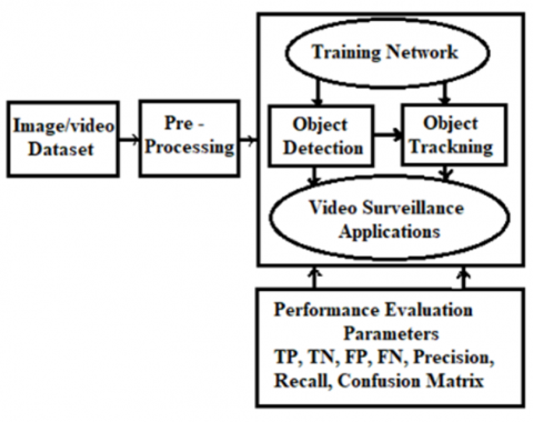
Moving object analysis, which is viewed as continuous identification of moving objects is an important execution. Moving object recognition is used to find varieties in pictures and whether there are variations, next removes the animated object. The moving object is distinguished by isolating the foreground object, that is to say, the moving object, along the fixed information perceived as background. Through video handling, the essential video is changed over into photo placements. Pretreatment is an underlying step that ought to be accomplished for the expulsion of noise in the pictures. The image will additionally be improved by pretreatment procedures. Include extraction is a methodology for catching the visual substance of pictures for indexing and retrieval. Highlight extraction is a sort of dimensionality decrease technique. Transforming the information to frame a gathering of features is known as the extraction include. The picked component ought to incorporate adequate information around the image with no other explicit information expected for their extraction. The picked component ought to be just to assess the chosen features. The features may be of either kind like tone, shape, and so forth. There are different element extraction strategies; principal component analysis, Gabor channel, string code character shape histogram, gray level co-occurrence matrix (GLCM), and so forth are a few of the element extraction systems. Extricated features are arranged as required. There are different classification approaches such ANNs, a classifier may be prepared relying upon requests. These may be neurons prepared relating to inputs and may be basically adjusted according to rules chose for classification. Over ongoing years, regions, for example, picture analytics with visual analytics have acquired a great many purposes. Spectral analysis with AI is two significant innovations that hang out in particular logical gatherings. There are late endeavors to address and mimic the visual vision of people, where the individual vision is the normal, substantial, and fathomable feeling of the person, with the development of an impression of the three-layered outside world [11, 12]. Human intelligence has been arranged over the course of the years to perceive and handle scenes caught by the eyes. These senses are at the center of most innovations. Ongoing exploration is currently uplifting researchers to uncover more nuances in the formation and information on pictures. Such progressions are because of top tier advancements, for example, CNN innovation. The applications given from Internet (Google, Facebook, and Snapchat) overall are among the ramifications of the enhancement in personal computer (PC) delivering and uses of deep learning methods. Through time-lapse, vision-based development has transformed from a discovery just philosophy to a shrewd handling structure that might get this ongoing reality. PC vision applications type moving way, observing, and autonomous moving object direction for object recognition and follow-up as significant hardships. For vehicles with other genuine objects, video surveillance is an interesting environment. In certain examinations, powerful calculation is a devoted utilization of body area and follow-up video surveillance in a perplexing environment [13, 14]. The application field of object area and tracking centers indivisibly around per PC vision applications. Where shape recognition is to perceive the component or track down the event of interest in assembling the thought frames. Where the object is molded by a novel directional strategy or technique to catch the shape in the incidental edges. The picture got from the dataset has various edges. Where the fundamental box chart of component recognition and its spin-off is displayed in Figure 2. The information set is isolated into twofold segments. 80% of the pictures in the dataset are utilized for planning and 20% for assessment. Picture recognition is additionally finished to follow the shapes in it utilizing CNN procedures estimations with YOLOv3. The leap box is created along the figure versus the over-interface (IoU) >0.5. The perceived bob box is sent as a source to the cerebrum networks that help it to get tracking. Limited edges are followed at the same time utilizing multi- object tracking (Adage). The meaning of such investigation mission is utilized in registering traffic thickness at heavy traffic convergences, in independent vehicles to distinguish different sorts of components with fluctuating enlightenment, additionally in optimizing smart city and smart vehicle systems [11-15].
Figure 2. Object recognition and tracking block diagram [15]
1.2 Object recognition and tracking
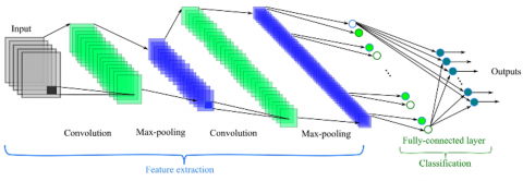
There is a capacity of computer vision functions that assist society, such as thing description, tracking, recognition, image annotation, counting, semantic segmentation. Interacting with things highlighted in the image and observing their location is recognized as thing recognition. Many UAC thing recognition tasks as presented in Figure 3. Along the advances in AI-assisted computer vision, task recognition has become possible along the time scale. Semantic segmentation function for clustering pixels based on similarity. The order localization and thing recognition strategy work to distinguish the shape category and unambiguously identify the bouncing box of its composition. State partitioning is a semantic partitioning applied to multiple objects [12-20]. Hence, among programmed object recognition, face reconstruction plans have been broadly examined, because of their likely employed, in numerous down-to-earth frameworks, for example, video observation, biometrics, also connection regulation frameworks amidst alternatives, those are powerfully reliant upon a precise face recognition. The face is a biometric personal trademark including significant info around the individual's personality. Consequently, an exact face reconstruction is the primary stage in numerous implementations, as example, face acknowledgment, face picture recovery, facial following, video observation, and so on. There are two methodologies utilized for face recognition which will be broke down: the handcrafted based-face identifiers as well as the ANNs-based face indicators. As explained in the previous sections, object recognition and tracking are achieved through a combination of technologies, as well as characteristics detection and matching, things classification and tracking. characteristics detection and matching involve extracting characteristics from a thing or site, such as lines and shapes, and contrast those characteristics with data from a database. In this part, we will review some of the most important techniques, algorithms and methods used to recognize objects, track and detect their features [16-25].
Figure 3. Various UAC object detection and recognition mechanism [18]
1.2.1 CNN structure
CNN is a kind of feed forward of ANN such that the singular neurons are brick in such a manner which they return to covering zones in the visible field. Along the first investigations, it is realized that the visual cortex includes an intricate plan of neurons. Such neurons are sensitive to little sub-zones of the visible area, named a responsive area. The sub-regions are tiled to covering the whole visible area.
These neurons operate as nearby filters along the data domain as well as are appropriate to take advantage of locally neighborhood relationship illustrated in regular pictures. Another studies, recently computes schemes relied upon such nearby networks among neurons and on progressively coordinated transformations of the image. In this work, it has been recognized that whenever neurons against the exact parameters are employed upon splatters of the last layer at various locations, a type of transitive invariance is accomplished. As per this thought, LeCun designed and prepared CNNs utilizing the blunder slope against back-proliferation calculation, acquiring state-of-the art execution on lots of example acknowledgment tasks [17-25]. Part of the fundamental improvements of CNN on neural network zone is the execution of substances allocating, applying identical loads on similar element plan that advances the training effectiveness by significantly diminishing the quantity of qualified components. Next, at that point, lately, dynamic functions with dropout computations were executed on CNN, that advances the non-linearity with autonomy of component plans, next, at such point, tends to larger-understanding with further stable features gained. In dependence on proceeding as a start to finish structure, many researches illustrate that the profound learning features inside the model might further being utilized as features to take UAVs of towards classification filters to lead PC visual missions, that is similar against conventional hand-make features. Contrasted against conventional pattern extraction with PC visual techniques, CNNs needs little pre-processing. Specifically, the system is subjected for training filters which is hand-designed in conventional techniques.
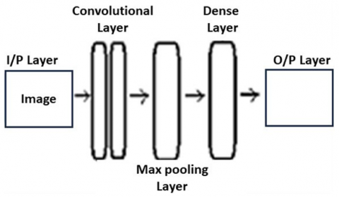
Contrasted against remaining trouble against design hand-designed features, the autonomy on earlier data is a significant advance of CNN. There are dual basic layer kinds in a CNN: convolutional layers with pooling layers. Also, against the advancement of CNN, dynamic utilities, fells are summed in request to ascend the inclusion of CNN. What's further, in the last layer of CNN, unique loss layers are select by the sort of missions. It will briefly make sense of all components that implemented in such study. Figure 4 displays a configuration of CNN complete model [18-26]. The bounds of the convolutional layer are made up of a set of learnable filters, which are sparse locally. During advanced access, each filter is transformed by the depth and level of the information field, providing two-layers legislation plan for such a filter. The network learns which filters will be triggered by certain types of features along contributing to certain locations, which is similar to convolutional activity in traditional striped algorithms-scraping key features from doorways.
Figure 4. General construction of CNN algorithm model [22]
A. Convolutional layer
Convolutional layer is a center structure block of CNN, that alters CNN against customary ANNs. To stay away along the direction of training billions of components (on the off chance that all layers are completely associated), using convolutional operations on limited territory has been illustrated. One significant benefit of convolutional networks is the substances participating in convolutional layers, as well as that known as carrying out similar filters on equivalent element plane. Loads participating assists to diminish the expected computing storage also to further develop CNN execution on PC vision missions. Figure 5 illustrates the substances participating impact on boundary decrease. Then, by lessening the quantity of qualified components, the past-meeting issue of customary neural network was satisfied [18-26]. Then loading these run plans for each filter on the depth side frames the overall size of the result. With the help of load sharing, the pool of trained filters in the convolutions has been expanded, enabling more information to be recognized on the input data. In a convolutional layer, a characteristic scheme is gotten by renew utilize of a capacity over sub-areas of the whole picture, all in all, by convolution of info picture against a filter, summing a predisposition term.
Figure 5. Demonstration of the convolutional layers versus fully combined weight sharing for the CNN algorithm [25]
In the event that we mean the k -th entered aspect guide of a certain convolutional layer as $h^k$, whose filter is designated as $W^k$ with predisposition is $b^k$, next the outcome feature guide of such convolutional layer $h^{k^* l}$ is gotten as:
$h^{k^* I}=W^k * h^k * b^k$ (1)
Such that, (*) represents the convolutional activity. For completely associated layer, it is an extraordinary instance of convolutional layer. A completely associated layer is a convolutional layer which catches every neuron in the past layer as well attaches them to each individual neuron it has, that is applying a convolutional layer beyond parameters allocating with each filter of such layer is using size 1×1. The essential operation of totally linked layer is to minimize the locally neurons positioned as well as along huge-perception features. A general mechanism to perform the mission is to use a CNN along the image. CNN handles image corrections to complete the task that may be obtained by region proposal networks, such as region convolutional neural network (RCNN) and fast region convolutional neural network (Fast-RCNN). To perform a specific object recognition task, a hierarchical clustering algorithm is used. Barely any bottlenecks with such methodologies are eliminated by best-in-class computations like the You Only Look Once (YOLO), Single Shot Detector (SSD). It is the professional object recognition computation that ensures a bounce box is given to all objects of distinct size to be perceived, in exchange for amazing computational capabilities, and faster processing. Serious consequences an SSD is guaranteed to deliver promising results; however, it has a trade-off between speed and accuracy. Thus, account identification is an explicit implementation [18-26]. Assuming the inputs in vectors to the network are denoted by; $X=\left[x_1, x_2, \ldots, x_l\right]^T$, the output layers represented by; $Y=\left[y_1, y_2, \ldots, y_k\right]^T$ with the prototypical for the optimization formulated as; $X: h \rightarrow Y$. The target datasets and its addictive noise might respectively being represented as; $\left[t^1, t^2, \ldots, t^k\right]$ with $u=\left[e^1, e^2, \ldots, e^k\right]$, the eccentric K denotes the overall network patterns with the associated vectors represented as; $V=\left[v_1, v_2, \ldots, v_{k-1}\right]$. The training algorithm is modeled with the following constraints when the training epochs are set to 1000 and the objective error is 0.001.
$\min _{h, w} \frac{1}{k} \sum_{j=1}^k\left(t^j-y_2^j\right)^2$ (2)
For forward and backward propagation, fully connected CNN employ the following formulations:
$x_j^{T+1}=\sum_i w_{j, i}^{T+1} x_i^T$ (3)
$g_j^{T+1}=\sum_i w_{j, i}^{T+1} g_i^T$ (4)
where, $w_{j, i}^{T+1}, \mathrm{~g}_j^T$ and $x_j^T$, are respectively, the weight connecting unit i at layer T to unit j at layer T+1 and the gradient and activation of unit I at layer T. The formulations above indicate that the activation units and gradients are pooled by the lower layer units connected to them and the higher layer units connected to them. However, due to the fact that connections leaving every piece are not constant lane of border effects, the pooling strategy becomes extremely painful and difficult to implement whenever calculating the gradients of the CNN. By dragging the incline from the upper layer, our model addresses this issue, and the CNN might be discriminately trained using the back propagation algorithm. A stochastic gradient decline might be utilized to update influences, as our formulation below demonstrates;
$w_{i, j}(t+1)=w_{i, j}(t)+\mu \frac{\partial C}{\partial w_{i, j}}$ (5)
The cost function, which is heavily influenced by factors like the learning type and the activation function, is located between C and the learning rate. The activation function and cost function, respectively, are the softmax and cross entropy functions, and this study is being carried out using supervised learning on a multiclass classification problem. The following is a definition of the softmax function:
$P_j=\frac{\exp \left(x_j\right)}{\sum \exp \left(x_k\right)}$ (6)
The unit j is the output that indicates the class probability, and the total inputs to units k and j of the same level are presented. The problem for multiclass classification in supervised learning is the cost function, which is well-defined as follows:
$C_r=\sum_j d_j \log \left(P_j\right)-v_j$ (7)
The weight is then linked to the preference unit in the unseen layer, and is the target probability for the output j. Weight is used to begin at the output unit, and error signals are transmitted value the input layer in a recursive fashion. As a cost function for the estimated error in the network's targeted function, the detected output compares favorably to the target valued, which was the facial image of the entire training set. The required minimization error is as follows:
$E^T=\frac{1}{2} \sum_{k=1}^K\left(t_k^T-\mathrm{g}_k^T\right)^2$ (8)
Such that, $E^T$ is the resulting error, $\mathrm{t}_{\mathrm{k}}^{\mathrm{T}}$, is the matching target value of the detected output (the activation of the kth output unit) is where the error is well-defined, $\mathrm{g}_k^T$.
B. Pooling layer
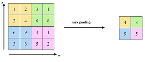
Pooling layer is regularly embedded among convolutional layers intermittently in a CNN structure. The capacity of pooling layer is to diminish the goal of feature maps, in this manner accomplishing spatial invariance as well as lightening the over-fitting issue [19-26]. In a pooling layer, each pooled feature map relates to a feature guide of the past layer. A little n × n patch, as illustrated in Figure 5, is utilized to join units of the feature plan, hence making location invariance along bigger neighborhoods. At the same time, it provides down examples of the contribution of n × n element along each direction. The maximum pooling strategy applied to the CNN pooling layer is illustrated in Figure 6 [18-26].
Figure 6. The maximum pooling technique utilized in CNN pooling layer [26]
Despite of mean pooling was regularly utilized in conventional CNN, maximum pooling has illustrated a superior execution in tests with is broadly utilized in ongoing CNN architecture plans. The outcome illustrates that maximum pooling is better than sub-examining for invariance catches in picture similar information. In addition, maximum pooling empowers quicker union rate by picking prevalent invariant features that further develops execution in speculation what's more, decreases the quantity of teachable boundaries, in this manner limiting estimations and processing time, bringing about a superior efficiency during preparing. Maximum pooling layer must satisfy the following formula:
$a_j=\max \left(a_i^{n \times n} u(n, n)\right)$ (9)
where, u(n, n) is the input data applied window that utilized to excerpt the ultimate value in the neighbored pixels data.
C. The activation function
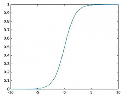
Using CNN, part of the almost important aspects is the execution of active function. Active functions increment the non-linearity in frameworks that prompts huge comprehension of the info group. Notwithstanding non-linearity, active function likewise provides out a feature plan beyond outrageous information amounts, which expands the independency of neurons in next layer, hence, at such point, outcomes increment the security of the entire network. Several utmost commonly involved active formulas in CNN are presented here. Unique significant normal affirmation is that each effective utilities ought to be differentiable, that guarantees the utilize of back-propagation technique in the preparation interaction. The activation function might be represented by what called sigmoid function as below [19-26]:
${sigm}(x)=\frac{1}{1-e^{-x}}$ (10)
The sigmoid function has been illustrated in Figure 7.
Figure 7. Graphical diagram of a typical sigmoid activation function [26]
D. Leakage
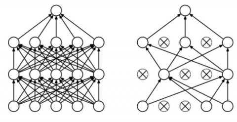
A CNN structure includes multiplexed non-straight hidden layers that compose CNN as dramatic scheme which might become familiar against the convoluted connections among the information sources and results. Notwithstanding, under the circumstance whereas there is restricted preparation information, large sums of such muddled connections will be the consequence of testing clamor, that only available in the preparation sets yet not in test information, regardless of whether the examining information is drawn along a similar dissemination. Then, at that point, over fitting would happen during preparing operation. Numerous techniques have been created to diminish such issue, such as halting the preparation whenever execution on an approval set begins to get more awful, presenting various weights punishments and delicate weight sharing sorts. Dropout is a strong calculation acquainted with take UAVs of the over fitting issue, which diminishes the speculation mistake of enormous brain systems. It diminishes complicated co-transformations of neurons, since in leakage calculation a solitary neuron can't depend on the presence of various neurons. Dropout, consequently, upgrades CNN to be capable to learn further vigorous features with balanced construction [27]. The term dropout alludes to exiting units (hidden and apparent) in a brain network. By rejecting a cell out, that mean briefly eliminating it along the system, alongside it everything associations [28]. A typical leakage diagram is illustrated in Figure 8 [19-26].
Figure 8. Graphical chart of a common dropout operation [26]
Actually, there are some drawbacks through the implementation of the CNNs that might be taken into consideration whenever employing such algorithms especially in patterns recognition and object recognition fields. The utmost necessary drawback in employing CNN algorithms is the requirement of further details and more data, which is an important condition in order to achieve superior performances. By other words, the further info entered to the CNN algorithm, the further efficient and accurate results will be obtained. Therefore, CNNs are considered as complicated techniques that consume huge sum of calculations and processing. This will be extremely expensive for training data because of the complicated info models. Furthermore, CNNs techniques require expensive machines hardware’s which will definitely increase the overall charge. As a summary of the proposed CNN algorithm, the advantages and disadvantages are reviewed in Table 1 [19-26].
Table 1. Advantages and drawbacks of the CNN algorithm [19-26]
|
Algorithm |
Advantages |
Disadvantages |
|
CNN |
1. Low dependency upon preprocessing operation of data. 2. Reducing the demands for human efforts and actions. 3. Simple in implementation. 4. Fast processing. 5. Highest accuracy among all image prediction techniques. |
1. Large computations expense 2. High cost 3. High complexity |
1.2.2 The gray level co-occurrence matrix
The gray level co-occurrence matrix (GLCM) technique is a statistical approach for feature extraction. Features are crucial item of objects data. By separate the feature, the processing period as well as the complication will be minimized. The spatial relationship of pixels is taken in an account to extract features. The image co-occurrence matrix might be determined utilizing GLCM. Pixels relation against other pixels might be specified in terms of distance and angle. The rows and columns number in a matrix is equal to the sum of grayscale levels in the GLCM matrix. GLCM format for the scaled image N × N is:
$\begin{aligned} & P_{i, j}(i, j) =\sum_{i=1}^N \sum_{j=1}^N 1, I(x, y), \text { and } I(x+\Delta x, y+\Delta y)=j, 0, { Otherwise }\end{aligned}$ (11)
where, p(i, j) indicates the co-occurrence joint probability at an offset (Δx, Δy) with spatial locations x and y also having a strength i and j. The length as well as the angle among the pixels to its territories are determined by the (Δx, Δy) offset. The number of distinct gray levels in the quantitative picture is indicated by G. In fact, pi(i) and pj(j) indicates the marginal probability matrix. Many features are determined by the following symbols:
$P_i(i)=\sum_{j=1}^G P(i, j)$ (12)
$P_j(j)=\sum_{i=1}^G P(i, j)$ (13)
A. The mean value
The mean values are denoted by μi and μj, micrometer. This provides the subscription of individual pixels density for the total picture [20-27].
$\mu_i=\sum_{i=1}^G P_i(i)$ (14)
$\mu_j=\sum_{j=1}^G P_j(j)$ (15)
B. The standard deviation
The standard deviation might be expressed by:
$\sigma_i=\sum_{i=1}^G\left(i-\mu_i\right)^2 P_i(i)$ (16)
$\sigma_j=\sum_{j=1}^G\left(j-\mu_j\right)^2 P_j(j)$ (17)
C. The variance
The variance is used to observe how each pixel varies along the adjacent pixel and it is utilized to classify various areas.
$Variance =\sum_{i, j}\left(P(i, j) \frac{1}{N}\right)^2$ (18)
D. The entropy
Entropy is a measure of the spatial disturbances within a picture. For example, if the info is organized, the entropy will be little amount.
$Entropy$ $=-\sum_{i, j} P(i, j) \log (P(i, j))$ (19)
E. The energy
The energy is opposite to entropy since it is utilized to estimate the local homogeneity. Energy will find the uniformity of the text.
$Homogeneity =\sum_{i=0}^{G-1} \sum_{j=0}^{G-1} \frac{P(i, j)}{1+(i-j)^2}$ (20)
F. The correlation
The correlation feature is a measurement of the linear dependency gray tone in the picture ad it is expressed by the following expression:
$Correlation =\sum_{i=0}^{G-1} \sum_{j=0}^{G-1} P(i, j) \frac{\left(i-\mu_i\right)\left(j-\mu_j\right)}{\sigma_x \sigma_y}$ (21)
G. The contrast
The contrast is specified as the local gray level alternation in the intensity of a pixel, which might be given by the expression:
$Correlation =\sum_{i=0}^{G-1} n^2\left\{\sum_{i=1}^G \sum_{j=1}^G P(i, j)\right\},|i-j|=n$ (22)
The remaining contents of this study will be organized as follows. Section 2 introduces the necessary concepts and important background of the subject of UAV navigation control and moving target detection with neural networks in terms of literature review of the most recent papers and related studies. Section 3 presents the design details and adjustments concerning the suggested model with illustration charts with discussions. Next, the simulation results and outcome signals will be displayed in Section 4. Finally, conclusions and future works will be outlined in Section 5.
1.3 Environmental effects
In fact, the effects of target height and weather changes are simulated by projecting them onto the data resolution, clarity, and contrast of captured images, thereby affecting the accuracy of the convolutional neural network algorithm in detecting objects and image objects.
1.3.1 Data resolution
Impact: Low resolution makes characteristics less clear, which makes it more difficult to identify small or far-off objects (like drones in aerial photos). While high resolution enhances detection, it also raises the cost of computing.
Where to process: The input layer includes preprocessing (such interpolation) and resizing.
Feature extraction: If the resolution is too low, early CNN layers (like Conv1-3) lose fine detail.
1.3.2 Image clarity (blur/noise)
Impact:
Blur minimizes edge sharpness, weakening gradient-relied feature detection.
Noise (e.g., sensor noise) creates false activations in filters.
Where to Address:
Preprocessing: Denoising (e.g., Gaussian filters) or deblurring (e.g., GANs).
Convolutional Layers: Deeper layers (e.g., Conv4-5) may fail to capture distorted features.
1.3.3 Contrast (lighting conditions)
Impact:
Low contrast (e.g., fog, shadows) flattens pixel intensity differences, minimizing feature discriminability.
High contrast might oversaturate edges, causing false detections.
Where to Address:
Normalization: BatchNorm layers or histogram equalization in preprocessing.
Activation Functions: ReLU might suppress little-contrast features; alternatives like LeakyReLU assist.
1.3.4 Final conclusions
Early CNN Layers (Conv1-3): Most affected by resolution and clarity.
Mid/Late Layers (Conv4-FC): More sensitive to contrast and high-level feature loss.
Preprocessing is Critical: Normalization, denoising, and resolution scaling directly influence CNN robustness.
For UAV detection, high-resolution, clear, and well-contrasted images maximize accuracy, while data augmentation (e.g., simulating fog/noise) improves model generalization.
The remaining contents of this study will be organized as follows. Section 2 introduces the necessary concepts and important background of the subject of UAV navigation control and moving target detection with neural networks in terms of literature review of the most recient papers and related studies. Section 3 presents the design details and adjustments concerning the suggested model with illustration charts with discussions. Next, the simulation results and outcome signals will be displayed in Section 4. Finally, conclusions with future works recommendations will be outlined in Section 5.
Several of the important examination articles and papers which talked about the moving object tracking and discovery with utilizing deep learning methods have been gathered and investigated. Through such audit, the subject of moving target discovery will be likewise addressed and reenacted utilizing mobile robotic multipurpose activity movement and moving object tracking that will be surveyed with logical papers connected with such point to be momentarily summed up in the accompanying paragraphs. Brunner et al. [20], a few kinematic structures allowed the robot to deliver the turning point maneuver, that makes them to revolve past transmission. It is gainful to correlate the event of described robots which can the inside plotting to accomplish part of the sort of advantage as well as give multiple kinds of motion. The enunciated robots, versus tracks, for instance, could effectively control their security while guiding on unpleasant terrains. Norouzi et al. [21] presented the usage of the Fast-Marching-Tree (FMT), the sampling-based computation, to tackle the innovation planning of a wheeled-legs mixture robot. The motion of the robot adapts finest or most consistent depending on the terrain mentalities. such characteristics may possibly subject to either the patterns or the terrain creation. Some portion of these features is the tilt or terrain bent. The slop impacts the robot's orientation points (roll and pitch), that is main requirement to be esteem for soundness conservation. Coman et al. [22] introduced one more investigation of the synthetic aperture radar (SAR) target classification using deep learning strategies. In this task, the proposed model of the examination, and the dataset of the SAR target have been dissected, modified, and arranged with the help of deep learning algorithms. Sánchez-Ibánez et al. [23], realized the capacity of method present algorithms is in fact needed for such kinds of robots, as they could observe gain to that take advantages of their huge adaptability. In the matter of popular preparation, the author used a Chart Search calculation, Dijkstra, for designing access by simulation hardware, register that motion formed is perfect to proceed all aspects of its parts. Thus, the specialists of such review distribution proposed the use of a PDE assessment way to deal with respect the multi-motion plans using an equally cost capability at the immediate of planning. Agarwal et al. [24] examined the information augmentation inside meager sign models using deep learning strategies. This study talked about the information augmentation issue against scanty waveform structures which are used in the demonstrating of the moving target applications. The exploration has been progressed by introducing deep learning algorithms to add brilliant methods to the recommended model. Bergman et al. [25] proposed the maneuver of robots is inspected utilizing vision charts and cross-section diagrams. The last choice involves making Edges based on motion substitutions, ensuring that the subsequent way is plausible because of progress limits, especially while utilizing diagram search algorithms. These diagrams' cells or hubs could save components (static or dynamic) of data about the surface at their areas. This could be as elevation data. In 2020, Effati et al. [26] proposed the robot's motion positioning is the issue of investigation. Below are a part of the different motor and dynamic models that the researchers collected up in this review is drive by differential. The stand turning sweep of robots with front Ackermann directing and high-rise energy employment of slip guiding robots during turning movement are two cases of imperatives that are proper to way arrangement. Vagale et al. [27] algorithms that don't need map portrayal (progressed) and those that do (exemplary) have been presented as a charming division in robot development control. High level delicate registering and sampling-based algorithms are dealt with by the conventional methodology, which incorporates chart research techniques. Feng et al. [28] proposed SAR target categorization based the combination of the ASC parts model and deep learning calculation. The creators in this task, the proposed model of the review, have examined the issue of the SAR target classification by applying the integration of the ASC areas plot against the deep learning calculation. This examination will help in giving classifications to the moving target, contingent upon the execution of the deep learning strategies. Kamal et. al. [29] proposed present day approaches for mobile object calculations by applying radio frequency recognizable proof. In this task, the proposed model of the examination, the moving object will be distinguished and assessed through using frequency space investigation of the communicated radio transmissions. The research problem and research gap can be summarized as the difficulty of determining the high accuracy of deep learning algorithms for detecting autonomous aircraft, especially in real time, with the increase in the percentage of errors and dispersion with altitude and climatic conditions.
3.1 Methodology details
The proposed deep leaning technique devoted for moving target tracking and detection will be presented and investigated in details. The problem of moving target detection and tracking might be implemented using deep learning strategies such as CNN. The fast regional CNN (FRCNN) has been nominated as the proposed method for moving target detection and tracking. Deep convolutional nets as of late have essentially gotten to the next level object recognition and picture grouping precision. The proposed model moving target detection and tracking using AI techniques is designed and simulated with the assistance of MatLab2020b m. files scripts codes as shown in Figure 9.
Figure 9. The proposed UAV moving target detection and tracking using AI techniques model simulation with MatLab2020b m. files scripts
Referring to Figure 9, the tested data will be entered first to the suggested model through a motion filter block. This block will act as features filter that will provide the required target properties by choosing specific pixels maps from the features of the motion data. This stage is very important in describing and preparing the entered data input in order to classify the required target data. Next, the filtered data will be entered to the suggested regional convolutional neural network (RCNN) algorithm block or section. The suggested RCNN algorithm will operate to train the entered data and adjusting the values of the internal hidden layer weights according to the required moving target data provided by the features filter section. The inner weights will still update until the resulting data track the desired moving target data sets and capturing the moved object picture. The flow chart of the proposed FRCNN algorithm is illustrated in Figure 10.
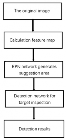
Figure 10. Flow chart of the proposed FRCNN algorithm
As presented in Figure 10, the structure of the flow chart will start with the original image reading section. The calculation of the features map will be accomplished in the second stage using features filters. Next, the suggested area of capturing will be generated using Region Processing Network section. Then the selected region will be entered to the detection network for target inspection comparison. Finally, after comparing the selected region with the target area, the results will be obtained and displayed in the detection results section. The construction of our proposed FRCNN algorithm is further demonstrated in Figure 11.
Figure 11. MatLab2020b design planning tool of the suggested FRCNN algorithm
Thus, by regarding Figure 11, this construction which has accomplished utilizing MatLab2020b application tools will provide the designer with powerful built-in functions to satisfy the details of the planned FRCNN flow chart. The necessary operational layers and functions inside the construction of the suggested FRCNN algorithm are introduced such as the input data layer, convolutional features filters layers, Relu functions, fully connected hidden layer weights, and SoftMax functions. These internal layers blocks and functions will construct the suggested deep learning FRCNN algorithm and specify its necessary operations for moving target detection. Moreover, the training of FRCNN Deep Neural Network classification has been analyzed as shown in Figure 12.
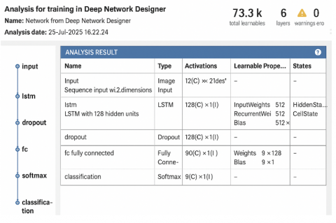
Figure 12. Analysis of testing the proposed designed FRCNN Deep Neural Network classification
By looking to Figure 12, one could observe the analysis tool which provides the necessary training examination to the designed deep neural RCNN network. The observed from the examination analysis that the suggested deep learning neural RCNN network will pass successfully without any errors, which indicates the success of the initial design of layers for the proposed algorithm using MATLAB tools to confirm the efficiency of its performance when implemented. Moreover, Table 2 illustrates the necessary parameters and design specifications utilized to adjust the operation of our suggested model implementation.
Table 2. Design parameters and specifications utilized to adjust the operation of the proposed model implementation
|
A |
B |
C |
D |
E |
F |
G |
H |
|
Training Options1 |
sgdm |
1 µ sec |
'piecewise' |
0.1 |
5 |
20 |
32 |
|
Training Options2 |
sgdm |
1 µ sec |
'piecewise' |
0.2 |
10 |
30 |
32 |
|
Training Options3 |
sgdm |
1 µ sec |
'piecewise' |
0.3 |
15 |
20 |
32 |
3.2 The employed datasets
In order to train the FRCNN network, several images will be tested containing information about safety conditions and prevention of moving target cases as described in the next paragraphs. The data sets have been obtained from Kaggle.com data store web site. The downloaded datasets containing of “561 Mbytes” with three groups, tested, training, and validation data. They consist of images of moving UAVs in various towns and streets with different marks. These data will train the FRCNN algorithm to be able of detecting any groups or individuals those who do not wear a protective mask, identify their photos and reveal their identities, are not committed to the conditions of prevention and safety.
In this Section, the proposed model for detecting and tracking moving targets using AI techniques was successfully implemented using the MatLab2020b m. Implement file script codes with necessary functions, modules and components, such as supporting functions, adaptive tuning algorithm tools and built-in utilities, with internal classes and important supporting simulation tools and functions. The results were achieved and presented in illustrative forms and organized tables, with a detailed discussion of each result achieved. Comprehensive discussions and scientific explanations were also provided for the recorded simulation results, comparing them to similar modern scientific studies and research.
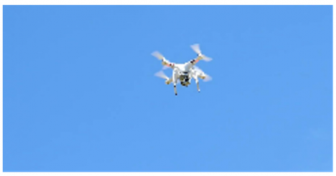
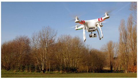
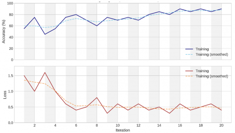
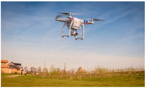
The program has been successfully implemented on a huge number of images downloaded from kaggle.com which contain details of face mask gathering groups persons. The Faster-RCNN algorithm was trained on a set of images of the needed object, those were selected to be the moving target sign, by choosing the square of the desired target area (object) and training the algorithm on it. The program has been executed many times on different image samples including various move UAVs details and upon the contents of a variety of surrounding, buildings, UAVs and roads to increase the accuracy of the algorithm in determining the target and enhance its efficiency. The figures presented below show the results of the practical examples of the program, such that, and thanks to God, were identical and with high accuracy, even reaching 95% applying the FRCNN technique. The first data picture test is for individual moving UAV target, that will enter to the FRCNN algorithm and trained among all tested data sets of various moving UAVs with various angles, and surrounding with different circumstances such as buildings, UAVs and roads. The first tested data picture entered to the suggested model is shown in Figures 13. Referring to Figure 13, we could observe the examination of the first input image which represents single moving coming UAV through road. We could recognize the tested moving Drone as the first target image to be examined by the suggested FRCNN algorithm. The training process of the implemented FRCNN algorithm has been obtained for the first test moving target Drone image as shown in Figure 14. From Figure 14, one could notice the progress of the implemented FRCNN algorithm accuracy curve appeared in the upper half of the figure with blue color. This accuracy curve starts from 20% and increased with the training epoch time to reaches 70% accuracy for the first image test. Also, we could recognize the error curve that appears in the lower half of the figure with red color which begun from 5 loss rate and reduced until it reaches to 1 loss error rate.
Figure 13. Examination of the 1st test image data
Figure 14. Training process of the implemented FRCNN algorithm for the first test moving Drone image
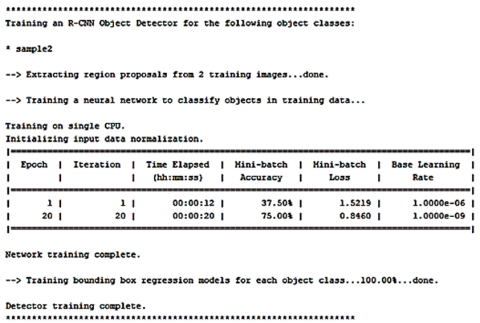
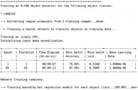
Also, the resulting statistics of the first tested image examination using the suggested FRCNN algorithm are presented in Figure 15.
By concerning the results achieved in Figure 15, we could observe the improved training accuracy from 37.5 to 75%, within 20 sect elapsed time, with epoch of 20, iterations of 20, minimum batch loss of 0.846, and base learning rate of 1*10-9, which indicates good accuracy results. Hence, the final obtained detected moving target image has been displayed in Figure 16 for the first tested data image.
Figure 15. The resulting statistics of the first tested image examination using the suggested FRCNN algorithm
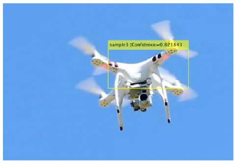
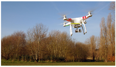
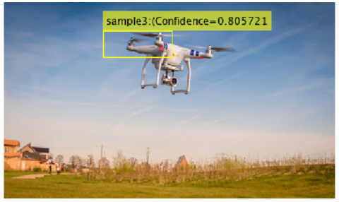
Thus, as illustrated in Figure 16, the final obtained detected moving target image has been presented with a frame box appears in yellow surrounding the moving part of the moving Drone image, which confirms the accuracy of the detection of the first examined data image from the trained data. Now, repeating the examination with the second data picture test of an individual second moving UAV target, which will entered to the FRCNN algorithm and trained among all tested data sets of various moving UAVs with various angles, and surrounding with different circumstances such as buildings, UAVs and roads. The second tested data picture entered to the suggested model is shown in Figures 17.
Figure 16. The final achieved detected UAV navigation control for moving target detection for the first tested data image
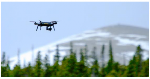
Figure 17. Examination of the 2nd test image data
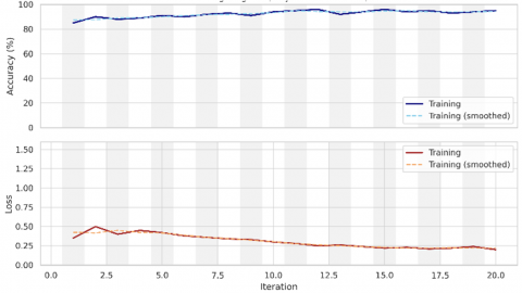
Referring to Figure 17, we could observe the examination of the second input image which also represents single moving outgoing UAV through road. We could notice the tested moving UAV as the second target image to be examined by the suggested FRCNN algorithm. The training process of the implemented FRCNN algorithm has been achieved for the second test moving target UAV image as displayed in Figure 18. From its figure, one might recognize the progress of the implemented FRCNN algorithm accuracy curve appeared in the upper half of the figure with blue color. This accuracy curve starts from 40% and increased with the training epoch time to reaches more than 80% accuracy for the second image test.
Figure 18. The obtained training process of the implemented FRCNN algorithm for the second test moving target UAV image
Furthermore, we could recognize the error curve that appears in the lower half of the figure with red color which begun from 1.5 loss rate and reduced until it reaches to 0.5 loss error rate. The resulting statistics of the second tested image examination using the suggested FRCNN algorithm are presented in Figure 19.
Figure 19. The resulting statistics of the second tested image examination using the suggested FRCNN algorithm
By concerning the results achieved in Figure 19, one could notice the improved training accuracy from 75.0 to 87.5%, within 12 sec elapsed time, with epoch of 20, iterations of 20, minimum batch loss of 0.5585, and base learning rate of 1*10-9, which indicates very good accuracy and fast training results. Now, the final achieved detected moving target image has been displayed in Figure 20 for the second tested data image. Thus, as illustrated in Figure 20, the final achieved detected moving target image has been presented with a frame box appears in yellow surrounding the most obvious part of the moving UAV image, which confirms the very good accuracy of the detection of the second examined data image from the trained data. Now, repeating the examination with the third data picture test of another two moving UAVs target data pictures, which will entered to the FRCNN algorithm and trained among all tested data sets of various moving Drones with various angles, and surrounding with different circumstances such as buildings, Drones and roads. The third tested data picture entered to the suggested model is shown in Figure 21.
Figure 20. The final obtained detected UAV navigation control for moving second tested data image
Figure 21. Examination of the 3rd UAV navigated test image data
Referring to Figure 21, one could observe the examination of the third input image which represents two moving opposite Drones. We could recognize the tested moving UAVs as the third target image to be examined by the suggested FRCNN algorithm. The training process of the employed FRCNN algorithm is achieved for the third test moving target UAV image as illustrated in Figure 22.
Figure 22. The achieved training process of the implemented FRCNN algorithm for the third test moving target UAV image
From Figure 22, the progress of the implemented FRCNN algorithm accuracy curve appeared in the upper half of the figure with blue color. This accuracy curve starts from 87.5% and increased with the training epoch time to reaches less than 75% accuracy for the third image test. Also, we might recognize the error curve that appears in the lower half of the figure with red color which begun from 0.55 loss rate and reduced until it reaches to 0.55 loss error rate. The resulting statistics of the third tested image examination using the suggested FRCNN algorithm are displayed in Figure 23.
Figure 23. The resulting statistics of the third tested image examination using the suggested FRCNN algorithm
By concerning the results obtained in Figure 23, we might see the decreased training accuracy from 87.5 to 75.5%, within 16 sec elapsed time, with epoch of 20, iterations of 20, minimum batch loss of 1.0805, and base learning rate of 1*10-9, which indicate good accuracy with fast training but confused results. Thus, the final obtained detected moving target image has been presented in Figure 24 for the third tested data image.
Figure 24. The final achieved detected UAV navigation control for moving the third tested data image
Thus, as demonstrated in Figure 25, the final obtained detected moving target image has been presented with a frame box appears in small yellow surrounding the most obvious part of the two moving UAVs image, which confirms the good accuracy but confused results for the detection of the third examined data image from the trained data.
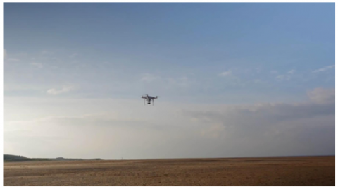
Figure 25. Exam of the 4th UAV navigated test image data
Moreover, repeating the examination with the fourth data picture test of another three moving UAVs target data pictures, which will entered to the FRCNN algorithm and trained among all tested data sets of various moving UAVs with various angles, and surrounding with different circumstances such as buildings, UAVs and roads. The fourth tested data picture entered to the suggested model is introduced in Figures 26. Referring to Figure 25, one might observe the examination of the 4th input image which represents three moving line rew UAVs. We could analyze the tested moving UAVs as the 4th target image to be examined by the suggested FRCNN algorithm. The training procedure of the employed FRCNN algorithm is obtained for the 4th test moving target UAV image as predicted in Figure 26.
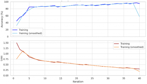
Figure 26. The achieved training process of the implemented FRCNN algorithm for the 4th test moving target UAV image
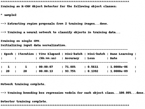
From Figure 26, one could notice the progress of the implemented FRCNN algorithm accuracy curve appeared in the upper half of the figure with blue colour. This accuracy curve starts from 70% and increased with the training epoch time to reaches about 90% accuracy for the 4th image test. Moreover, we might recognize the error curve that appears in the lower half of the figure with red colour which begun from 0.5 loss rate and reduced until it reaches to 0.2 loss error rate. Also, the resulting statistics of the 4th tested image examination using the suggested FRCNN algorithm are displayed in Figure 27. By regarding the results achieved in Figure 27, we might recognize the improved training accuracy from 71.88 to 93.75%, within 13 sec elapsed time, with epoch of 20, iterations of 20, minimum batch loss of 0.1292, and base learning rate of 1*10-9, which indicates an excellent accuracy with fast training results. Hence, the final achieved detected moving target image has been introduced in Figure 28 for the 4th UAV navigated tested data image.
Figure 27. The resulting statistics of the 4th UAV navigated tested image examination using the suggested FRCNN algorithm
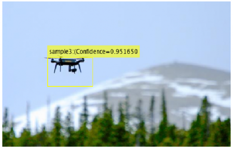
Figure 28. The final achieved detected moving target image for the 4th UAV navigated tested data image
Thus, as presented in Figure 28, the final achieved detected moving target image has been displayed with a frame box appears in large yellow surrounding the most obvious and nearest part of the three moving Drones image, which confirms the excellent accuracy results for the detection of the 4th examined data image from the trained data. Next, repeating the examination with the fifth data picture test of another moving Drone target data picture, which will entered to the FRCNN algorithm and trained among all tested data sets of various moving UAVs with various angles, and surrounding with different circumstances such as buildings, UAVs and roads. The fifth tested data picture entered to the suggested model is shown in Figure 29.
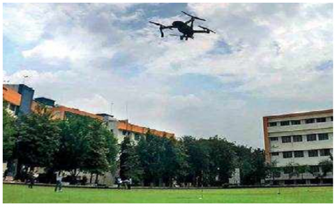
Figure 29. Examination of the 5th test image data
The training process of the employed FRCNN algorithm is achieved for the 5th test moving target UAV image as presented in Figure 30.
Figure 30. The process of the implemented FRCNN algorithm for the 5th test moving target UAV image
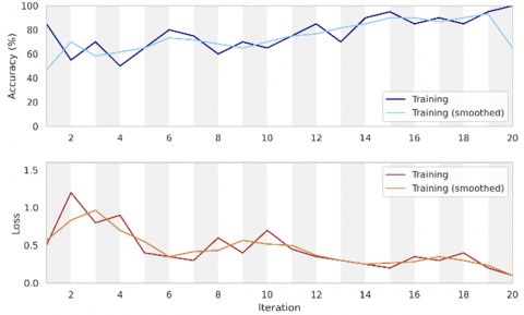
From Figure 30, we might notice the progress of the implemented FRCNN algorithm accuracy curve appeared in the upper half of the figure with blue colour. This accuracy curve starts from 40% and increased with the training epoch time to reaches about 90% accuracy for the 5th image test. Furthermore, we could observe the error curve that appears in the lower half of the figure with red colour which begun from 2 loss rate and reduced until it reaches to 0.25 loss error rate. Moreover, the resulting statistics of the 5th tested image examination using the suggested FRCNN algorithm are presented in Figure 31.
Figure 31. Resulting statistics of a 5th UAV navigated tested image examination using the suggested FRCNN algorithm
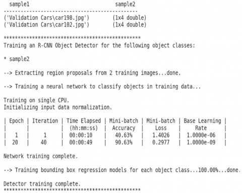
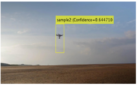
By considering the results displayed in Figure 31, one could notice the improved training accuracy from 40.63 to 99.63%, within 49 sec elapsed time, with epoch of 20, iterations of 20, minimum batch loss of 0.2977, and base learning rate of 1*10-9, which indicate an excellent accuracy with slow training results. Thus, the final obtained detected moving target image has been introduced in Figure 32 for the 5th tested data image. Thus, as illustrated in Figure 32, the final obtained detected moving target image has been introduced with a frame box appears in small yellow surrounding the most obvious and nearest part of the moving UAV image, which confirms the excellent accuracy but slow training results for the detection of the 5th examined data image from the trained data. At last, repeating the examination with the sixth data picture test of another moving UAV target data picture, which will entered to the Faster RCNN algorithm and trained among all tested data sets of various moving Drones with various angles, and surrounding with different circumstances such as buildings, drones and roads.
Figure 32. The final achieved detected UAV navigation control for the 5th moving tested data image
The 6th UAV tested data picture entered to the suggested model is shown in Figure 33.
Figure 33. Exam of a 6th UAV navigated test image data
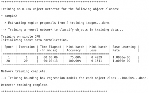
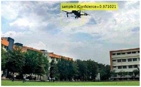
The training process of the employed FRCNN algorithm is analysed for the 6th test moving target UAV image as illustrated in Figure 34. In this Figure, one could recognize the progress of the implemented FRCNN algorithm accuracy curve appeared in the upper half of the figure with blue colour. This accuracy curve starts from 75% and increased with the training epoch time to reaches more than 95% accuracy for the 6th image test. Also, we might see the error curve that appears in the lower half of the figure with red colour which begun from 0.5 loss rate and reduced until it reaches to 0.1 loss error rate. Furthermore, the resulting statistics of the 6th tested image examination using the suggested FRCNN algorithm are presented in Figure 35. By regarding the results shown in Figure 35, we might observe the improved training accuracy from 75 to 100%, within 13 sec elapsed time, with epoch of 20, iterations of 20, minimum batch loss of 0.1611, and base learning rate of 1*10-9, which indicates the utmost better and excellent accuracy with fast training results. Thus, the final achieved detected moving target image has been introduced in Figure 36 for the 6th tested data image with a frame box appears in yellow surrounding the most obvious and nearest part of the moving UAV image, which confirms the excellent accuracy but slow training results for the detection of the 6th examined data image from the trained data.
Figure 34. The achieved training process of the implemented FRCNN algorithm for the 6th test moving target UAV image
Figure 35. Resulting statistics of a 6th UAV navigated tested image examination using the suggested FRCNN algorithm
Figure 36. The final achieved detected moving target image for the 5th UAV navigated tested data image
Finally, we might conclude that robust implementation has been achieved for moving target detection and tracking simulation using efficient deep learning FRCNN algorithm updated by applying MATLAB and tested on a set of data for images of various moving wheels. The results of several tests showed the success of the applied algorithm design in identifying and detecting moving targets with a high accuracy of more than 93% and a small error rate of 0.01 with a good training speed for the tested data set of 12 seconds.
In addition to the results obtained in this chapter, the proposed model of the proposed Artificial Intelligence technology FRCNN was used to detect and track moving targets with high efficiency and a low error rate, in addition to achieving a good training speed by testing sets of experimental data and entering them into the layers of the proposed algorithm using MATLAB m. files scripts codes. In this thesis, and through the results achieved for the system and the smart technology used, we can summarize the advantages and disadvantages, or the so-called strengths and weaknesses, to provide the reader with a final conclusion and a general review of the quality of the proposed model, as shown in Table 3.
Moreover, we could compare our achieved results with other detection techniques, as shown in Table 4.
Table 3. Advantages against drawbacks of the proposed UAV navigation using modified NNsl
|
Advantages |
Drawbacks |
|
-Robust deep learning implementing with high efficiency of >93% |
-Reduced efficiency in distinguishing multiple moving targets at the same time |
|
-Very good min. batch loss = 0.01for epochs time = 20 |
-Increased training time in multi-target data tests, slow access and convergence of results |
|
-Min. Training time =12 sec |
-The need for a fast processor to achieve real time implementation |
|
-Improved deep learning FRCNN algorithm implementation with low cost |
-Increasing the effort of calculations, especially with increasing accuracy of the entered data, especially in shooting data for rapidly moving targets |
Table 4. Comparison of our achieved results with other detection techniques
|
Model |
Performance |
Error Rate |
Accuracy |
Delay (Inference Speed) |
Notes |
|
CNN |
Moderate |
Medium-High |
Moderate |
High (Slow) |
Good for feature extraction but slower for real-time. |
|
YOLO (v5/v8) |
High |
Low-Medium |
High |
Low (Fast) |
Optimized for real-time, balances speed/accuracy. |
|
SSD |
High |
Medium |
High |
Medium |
Faster than CNN but slightly less accurate than YOLO. |
|
Transformers (DETR) |
Very High |
Low |
Very High |
High (Slow) |
High accuracy but computational heavy. |
An air UAV surveillance system for navigation control and monitoring devices which operates with smart technologies to detect moving targets was proposed. The ANNs trained utilizing the developed Levenberg-Marquardt technique that are used to automatically recognize and classify moving targets in the advanced radar system. The data of the moving object through reflected radar signals is fed into the training module of the AI system, which trains the AI algorithm to plot and track the path of the moving object based on the reflected radar signals. In this study, we conclude that a robust implementation of moving target detection and tracking simulation has been achieved using an efficient deep learning FRCNN algorithm that has been updated by implementing MATLAB and tested on a dataset of different moving wheel images. The results of several tests showed the success of the applied algorithmic design in identifying and detecting moving targets with a high accuracy of more than 93% and a simple error rate of 0.01, with a good training speed for the tested data set of 12 seconds.
[1] Alonso-Mora, J., Breitenmoser, A., Rufli, M., Beardsley, P., Siegwart, R. (2013). Optimal reciprocal collision avoidance for multiple non-holonomic robots. In Distributed Autonomous Robotic Systems: The 10th International Symposium. Springer Berlin Heidelberg, pp. 203-216. https://doi.org/10.1007/978-3-642-32723-0_15
[2] Bera, A., Kim, S., Manocha, D. (2015). Efficient trajectory extraction and parameter learning for data-driven crowd simulation. Canadian Information Processing Society, Canada, pp. 65-72. https://dl.acm.org/doi/10.5555/2788890.2788903
[3] Bertinetto, L., Valmadre, J., Henriques, J.F., Vedaldi, A., Torr, P.H. (2016). Fully-convolutional siamese networks for object tracking. In Computer vision—ECCV 2016 Workshops: Amsterdam, the Netherlands, pp. 850-865. https://doi.org/10.1007/978-3-319-48881-3_56
[4] Brockman, G., Cheung, V., Pettersson, L., Schneider, J., Schulman, J., Tang, J., Zaremba, W. (2016). OpenAI gym. arXiv preprint arXiv:1606.01540. https://doi.org/10.48550/arXiv.1606.01540
[5] Xia, C., El Kamel, A. (2015). A reinforcement learning method of obstacle avoidance for industrial mobile vehicles in unknown environments using neural network. In Proceedings of the 21st International Conference on Industrial Engineering and Engineering Management 2014, Tianjin, China, pp. 671-675. https://doi.org/10.2991/978-94-6239-102-4_136
[6] Cova, T.J., Johnson, J.P. (2003). A network flow model for lane-based evacuation routing. Transportation Research Part A: Policy and Practice, 37(7): 579-604. https://doi.org/10.1016/S0965-8564(03)00007-7
[7] Curtis, S., Manocha, D. (2013). Pedestrian simulation using geometric reasoning in velocity space. In Pedestrian and Evacuation Dynamics 2012. Springer International Publishing, USA, pp. 875-890. https://doi.org/10.1007/978-3-319-02447-9_73
[8] Dung, L.T., Komeda, T., Takagi, M. (2008). Reinforcement learning for POMDP using state classification. Applied Artificial Intelligence, 22(7-8): 761-779. https://doi.org/10.1080/08839510802170538
[9] Fiorini, P., Shiller, Z. (1998). Motion planning in dynamic environments using velocity obstacles. The International Journal of Robotics Research, 17(7): 760-772. https://doi.org/10.1177/027836499801700706
[10] Vagale, A., Oucheikh, R., Bye, R.T., Osen, O.L., Fossen, T.I. (2021). Path planning and collision avoidance for autonomous surface vehicles I: A review. Journal of Marine Science and Technology, 26: 1292-1306. https://doi.org/10.1007/s00773-020-00787-6
[11] Souissi, O., Benatitallah, R., Duvivier, D., Artiba, A., Belanger, N., Feyzeau, P. (2013). Path planning: A 2013 survey. In Proceedings of 2013 International Conference on Industrial Engineering and Systems Management (IESM), Agdal, Morocco, pp. 1-8.
[12] Yi, C.H., Jeong, S.D., Cho, J.W. (2012). Map representation for robots. Smart Computing Review, 2(1): 18-27. https://doi.org/10.6029/smartcr.2012.01.002
[13] Nash, A., Koenig, S. (2013). Any-angle path planning. AI Magazine, 34(4): 85-107. https://doi.org/10.1609/aimag.v34i4.2512
[14] Petres, C., Pailhas, Y., Petillot, Y., Lane, D. (2005). Underwater path planing using fast marching algorithms. In Europe Oceans 2005, Brest, France, pp. 814-819. https://doi.org/10.1109/OCEANSE.2005.1513161
[15] Huang, H.P., Chung, S.Y. (2004). Dynamic visibility graph for path planning. In 2004 IEEE/RSJ International Conference on Intelligent Robots and Systems (IROS), Sendai, Japan, pp. 2813-2818. https://doi.org/10.1109/IROS.2004.1389835
[16] Patel, N., Slade, R., Clemmet, J. (2010). The ExoMars rover locomotion subsystem. Journal of Terramechanics, 47(4): 227-242. https://doi.org/10.1016/j.jterra.2010.02.004
[17] Papadakis, P. (2013). Terrain traversability analysis methods for unmanned ground vehicles: A survey. Engineering Applications of Artificial Intelligence, 26(4): 1373-1385. https://doi.org/10.1016/j.engappai.2013.01.006
[18] Zhang, H.J., Zhang, Y.D., Yang, T.T. (2020). A survey of energy-efficient motion planning for wheeled mobile robots. Industrial Robot: the International Journal of Robotics Research and Application, 47(4): 607-621. https://doi.org/10.1108/IR-03-2020-0063
[19] Otsu, K., Matheron, G., Ghosh, S., Toupet, O., Ono, M. (2020). Fast approximate clearance evaluation for rovers with articulated suspension systems. Journal of Field Robotics, 37(5): 768-785. https://doi.org/10.1002/rob.21892
[20] Brunner, M., Fiolka, T., Schulz, D., Schlick, C.M. (2015). Design and comparative evaluation of an iterative contact point estimation method for static stability estimation of mobile actively reconfigurable robots. Robotics and Autonomous Systems, 63: 89-107. https://doi.org/10.1016/j.robot.2014.09.003
[21] Norouzi, M., Miro, J.V., Dissanayake, G. (2017). Planning stable and efficient paths for reconfigurable robots on uneven terrain. Journal of Intelligent & Robotic Systems, 87: 291-312. https://doi.org/10.1007/s10846-017-0495-8
[22] Coman, C. (2018). A deep learning SAR target classification experiment on MSTAR dataset. In 2018 19th International Radar Symposium (IRS), Bonn, Germany, pp. 1-6. https://doi.org/10.23919/IRS.2018.8448048
[23] Sánchez-Ibánez, J.R., Pérez-del-Pulgar, C.J., Azkarate, M., Gerdes, L., García-Cerezo, A. (2019). Dynamic path planning for reconfigurable rovers using a multi-layered grid. Engineering Applications of Artificial Intelligence, 86: 32-42. https://doi.org/10.1016/j.engappai.2019.08.011
[24] Agarwal, T., Sugavanam, N., Ertin, E. (2023). Sparse signal models for data augmentation in deep learning ATR. Remote Sensing, 15(16): 4109. https://doi.org/10.3390/rs15164109
[25] Bergman, K., Ljungqvist, O., Axehill, D. (2020). Improved path planning by tightly combining lattice-based path planning and optimal control. IEEE Transactions on Intelligent Vehicles, 6(1): 57-66. https://doi.org/10.1109/TIV.2020.2991951
[26] Effati, M., Fiset, J.S., Skonieczny, K. (2020). Considering slip-track for energy-efficient paths of skid-steer rovers. Journal of Intelligent & Robotic Systems, 100: 335-348. https://doi.org/10.1007/s10846-020-01173-5
[27] Taghavifar, H., Rakheja, S., Reina, G. (2021). A novel optimal path-planning and following algorithm for wheeled robots on deformable terrains. Journal of Terramechanics, 96: 147-157. https://doi.org/10.1016/j.jterra.2020.12.001
[28] Feng, S.J., Ji, K.F., Zhang, L.B., Ma, X.J., Kuang, G.Y. (2021). SAR target classification based on integration of ASC parts model and deep learning algorithm. IEEE Journal of Selected Topics in Applied Earth Observations and Remote Sensing, 14: 10213-10225. https://doi.org/10.1109/JSTARS.2021.3116979
[29] Kamal, A.E., Mahmood, Z.S., Nasret, A.N. (2022). A new methods of mobile object measurement by using radio frequency identification. Periodicals of Engineering and Natural Sciences (PEN), 10(1): 295-308.