Khaoula Talbi*![]() | Samia Harrouni
| Samia Harrouni![]()
© 2025 The authors. This article is published by IIETA and is licensed under the CC BY 4.0 license (http://creativecommons.org/licenses/by/4.0/).
OPEN ACCESS
Assessing solar energy potential is vital for developing solar conversion technologies. Despite Algeria's high solar capacity, the country faces challenges due to a limited number of meteorological stations that measure solar radiation (SR). This paper presents a study investigating the performance of innovative hybrid models (HMs) proposed to improve the SR estimation on inclined surfaces over 5-minute intervals. These HMs are formed by combining five empirical models (EMs) and five transposition models (TMs), resulting in a total of 25 models. The 25 HMs are applied to estimate the SR in two locations in Algeria, Bouzareah and Ghardaia. A comparative study is conducted in MATLAB, evaluating the performance of the suggested HMs and five EMs. The findings demonstrate that the HMs significantly enhance accuracy, particularly under cloudy conditions, reducing the normalized root mean square error (NRMSE) by up to 90% in some cases. For example, on August 16th in Ghardaia, the NRMSE decreased from 25% to 5.32% with our hybrid technique, demonstrating its superiority. Unlike traditional clear-sky models, our method performs well on overcast days. For example, on December 10th in Ghardaia, the Bird and Hulstrom model alone produced a high NRMSE of 35% with a KT value of 0.28; however, combining it with the Temps model reduced the NRMSE to 13.37%. In addition, the HMs based on Bird & Hulstrom-Temps provide the most accurate estimates at both locations, with coefficient of determination (R²) values from 0.9788 to 0.9992 and NRMSE values between 3.33% and 19.64%. In contrast, the Davis and Hay-Hay-based HMs offer the lowest R² values and the highest NRMSE and NMBE values.
solar radiation (SR), empirical models (EMs), estimation, transposition models (TMs), hybrid models (HMs), clearness index, statistical assessment
The spectral distribution of radiation reaching the Earth's surface is influenced by both the dispersal of radiation from outer space and the atmospheric constituents. The distribution of this phenomenon on land is of utmost importance in a wide range of applications, including earth-based solar power systems, the Earth's reflectivity, and photochemical reactions [1]. These applications require precise knowledge of solar resource availability in different regions [2]. In Algeria, the national energy plan emphasizes the rapid expansion of solar energy, particularly through the development of solar photovoltaic (PV) and solar power technologies. The government aims to launch multiple solar PV projects with a combined capacity of 800 MWp by 2020, with plans for additional projects with an annual capacity of 200 MWp from 2021 to 2030. However, accurately determining the distribution of solar radiation (SR) remains a challenge [3].
In regions where observed data is unavailable, it is customary to estimate SR using models, often classified into radiative transfer models [4], remote sensing retrievals [5], machine learning models [6, 7], and empirical models (EMs) [8, 9]. The EMs are widely used for SR estimation due to their low computational cost and their readily available inputs [10]. Among them are the models developed by Liu & Jordan, Perrin de Brichambaut, and Capderou. Various studies have utilized these models to estimate global, beam, and diffuse radiation across several regions in Algeria. For instance, Hamdani et al. [11] applied the Capderou, Perrin de Brichambaut, and R. Sun models to calculate hourly SR in Ghardaia, a city in the northern central region of the Sahara Desert of Algeria. Similarly, S-Koussa et al. [12] used the Bird & Hulstrom model to determine the three components of SR per hour in Ghardaia. Further, Benkaciali and Gairaa [13] applied both Liu & Jordan, and Brichambaut models to estimate daily and hourly SR at a specific location. Mesri-Merad et al. utilize several models, including Lacis & Hansen, Bird & Hulstrom, Davies & Hay, and Atwater, to compute hourly global SR (GSR) at two locations: Bouzareah in northern Algiers and Ghardaia [14]. Nia et al. [15] conducted a study using the Angstrom & Prescott model to assess monthly GSR across four cities in Algeria: Algiers, Oran, Bechar, and Tamanrasset. Bouramdane et al. [16] applied two semi-empirical methods to estimate daily inclined SR in Ghardaia. Their findings showed that the Liu & Jordan model produced more accurate results compared to experimental data, particularly at dawn and sunset. In addition, the Perrin de Brichambaut model proved to be the most suitable around solar noon. In another study, Lantri et al. [17] used available meteorological records to estimate different components of SR on a horizontal surface, concluding that Model 3 was the most accurate for estimating the global component based on relative humidity and water vapor tension. Soulouknga et al. [18] evaluated six EMs over 26 years of meteorological data from the Abeche site. Their results showed that the Sabbagh model provided the most accurate estimation, with excellent precision based on statistical indicators. EMs in the literature typically represent clear-sky conditions, leading to notable discrepancies compared to measured values, especially on cloudy days. Therefore, three models, Liu & Jordan, Capderou, and Perrin de Brichambaut, develop semi-EMs to estimate solar irradiance on horizontal surfaces. These models use consistent equations to convert data from horizontal to inclined planes, based on the well-known Liu & Jordan model from 1968. Since then, other transposition models (TMs) have emerged, offering enhancements to facilitate the transformation from horizontal to inclined planes, primarily differing in their treatment of the diffuse component.
From this survey, it can be observed that despite the availability of numerous estimation methods (EMs), only a few have been evaluated for short-term (5-minute) GSR predictions at Algerian sites. Given the inherently dynamic nature of SR, which can fluctuate significantly within minutes, and the critical need for real-time control and optimization in PV systems, 5-minute GSR estimation is crucial for ensuring their efficient and stable operation. Forecasts from a few seconds to a few minutes are necessary to manage rapid fluctuations and ramp rates, leading to smoother power production. This allows PV inverters, energy storage systems, and grid control equipment to adjust preemptively before cloud-induced power drops occur. A 5-minute resolution aligns with the response time of automatic grid control systems and helps prevent costly power quality issues, spinning reserve activations, and voltage fluctuations that can impact grid stability. For large PV installations, this results in measurable improvements in capacity factor, reduced curtailment losses, and enhanced grid integration capabilities, making it an essential tool for modern grid-scale PV systems [19, 20]. On the other hand, we note that EMs typically demonstrate the highest accuracy under clear-sky conditions; however, their precision diminishes significantly during cloudy periods, when SR exhibits the most variability. Furthermore, the performance investigation of hybrid models combining EMs with TMs has not yet been adequately explored in the literature. To address this research gap, this study investigates the performance of innovative hybrid models that merge five EMs with five TMs for predicting 5-minute GSR on inclined surfaces at two climatically diverse locations in Algeria: Ghardaia and Bouzareah. The main aim of the proposed method is to ensure an accurate estimation of the GSR on inclined surfaces. The paper’s key contributions are:
The remainder of the paper is structured as follows: Section 2 describes the proposed method and provides a comprehensive evaluation of five EMs and five TMs. In Section 3, the results of a comparative study evaluating the performance of the developed models are presented and discussed. Finally, Section 4 offers the main conclusions.
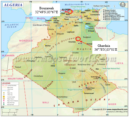
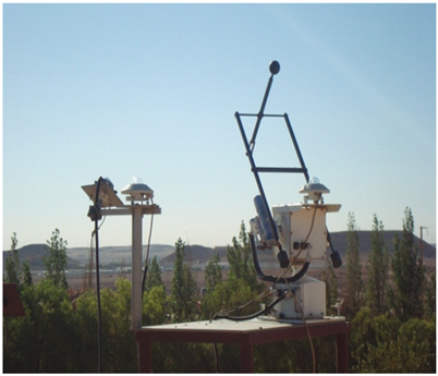
A data bank containing GSR measurements at 5-minute intervals is used to evaluate the effectiveness of the radiation models under study for two locations. The first site, Ghardaia, is located in the southern region of Algeria (Figure 1(a)). The Applied Research Unit for Renewable Energies (URAER) collected the data in 2006 on surfaces inclined at a 30° angle by using a radiometric station shown in Figure 1(b). The second site, Bouzareah, is situated in Algiers, in the northern region of Algeria (Figure 1(a)). The Renewable Energy Development Center (CDER) gathered the data there in 2013 on surfaces inclined at a 36.8° angle. Table 1 presents the geographic coordinates of the examined regions.
(a)
(b)
Figure 1. (a) Ghardaia and Bouzareah sites' location and (b) Ghardaia radiometric station (latitude 33°27'N, longitude 3°46'E, and altitude 463 m)
Table 1. Geographical locations of the sites under study
|
Site |
Latitude |
Longitude |
Altitude |
|
Ghardaia |
32°49'N |
03°67'E |
503 m |
|
Bouzareah |
36°78'N |
03°01'E |
226 m |
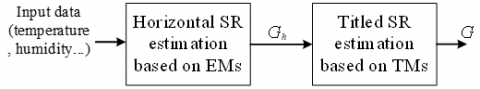
The global expansion of solar energy has underscored the imperative for an accurate and meticulous assessment of SR. Using only traditional models, such as empirical ones, may not be enough to achieve accurate estimation with high performance. Hybridizing these models with other models is a compelling approach to overcome the limitations of individual estimating models and enhance estimation accuracy. Figure 2 shows the developed HMs, which merge five empirical and five transposition models, resulting in 25 combinations, to predict GSR on inclined surfaces. Each HM consists of one EM and one TM. The EM estimates the horizontal GSR, Gh, from the input data, while the TM facilitates the conversion from a flat to an inclined surface and achieves the titled GSR, G. These HMs offer two significant benefits. First, it enables the application of TMs in cases where horizontal radiation data are unavailable, a common occurrence across many locations in Algeria, particularly in the expansive southern area. Second, it enhances the performance of EMs, leading to more accurate estimation. Note that the five EM and TM are selected due to their: i) simplicity and proven estimation accuracy, ii) extensive validation in prior literature for SR estimation in similar climates/regions [11].
The mathematical formulas of each EM and TM involved are given in the next subsections.
Figure 2. Schematic diagram of the HMs designed for GSR estimation on inclined surfaces
3.1 Empirical models
3.1.1 Capderou model
As Figure 3 depicts, the total radiation, G, incident on a surface with any given orientation is expressed as the sum of two components as follows [3]:
Figure 3. Solar radiation distribution
$G=I+D$ (1)
where, I and D denote the direct and diffuse radiations, which are defined below.
a) Direct radiation: The direct radiation on the inclined surface is expressed by:
$I=I_{S C} exp \left[-T_l\left(0.9+\frac{9.4}{(0.89)^z} \sin (h)\right)^{-1}\right] \cos (i)$ (2)
where, ISC is the solar constant, h is the sun height, z is the altitude, Tl is the link trouble factor, and i is the angle of incidence, for a horizontal plane is given by $\cos (i)=\sin (h)$.
b) Diffuse radiation: The diffuse radiation consists of three components as given in Eq. (3):
$D=D_1+D_2+D_3$ (3)
with:
$D_1=\delta_d \cos (i)+\delta_i \frac{1+\sin (\omega)}{2}+\delta_h \cos (\omega)$ (4)
where, the terms $\delta_d, \delta_i$, and $\delta_h$ refer to the direct or circumsolar, isotropic, and horizon circles, respectively, and $\omega$ denotes the hour angle.
$D_2=\delta_a \frac{1-\sin (\omega)}{2}$ (5)
where, $\delta_a$ defines the soil diffusion coefficient, and for a horizontal plane, the diffuse radiation from the ground is zero.
$D_2=\delta_a \frac{1-\sin (\omega)}{2}$ (6)
3.1.2 Liu & Jordan model
Liu & Jordan model define the general formula for GSR, G, received by a tilted surface comprising three components, as follows [15]:
$G=I_h \cdot R_b+D_h \cdot\left(\frac{1+\cos (\beta)}{2}\right)+\left(\frac{1-\cos (\beta)}{2}\right) \cdot G_h \cdot \rho$ (7)
In this formula, Ih, Dh, and Gh represent the direct, diffuse, and global radiation on a horizontal surface, respectively. The parameter β denotes the tilt angle, ρ is the ground albedo (reflectance of the ground), and Rb is the ratio of beam radiation incident on an inclined plane to that on a horizontal plane. For surfaces in the northern hemisphere that are south-facing, Rb is defined as:
$R_b=\frac{\cos (\varphi-\beta) \cos (\delta) \cos (\omega)+\sin (\varphi-\beta) \sin (\delta)}{\cos (\varphi) \cos (\delta) \cos (\omega)+\sin (\varphi) \sin (\delta)}$ (8)
where, $\varphi$ and $\delta$ are the latitude of the location and the declination angle of the sun, respectively.
For a horizontal plane, the GSR can be formulated as:
$G=G_h=I_h+D_h$ (9)
a) Direct radiation: The direct radiation on a horizontal surface $I_h$ is expressed as:
$I_h=A \sin (h) \exp \left(\frac{-1}{c \sin (h+2)}\right)=\frac{I}{R_b}$ (10)
where, I is the direct radiation on a tilted surface at an angle β.
b) Diffuse radiation: The diffuse radiation Dh is determined by:
$D_h=B(\sin (h))^{0.4}$ (11)
In Eqs. (10) and (11), A, B, and c are constants that take into account the nature of the sky [16].
The reflected radiation on a tilted surface, R, is given by:
$R=\left(I_h+D_h\right)\left(\frac{1-\cos (\beta)}{2}\right) \rho$ (12)
For a horizontal plane, the value of the reflected radiation is zero [16].
3.1.3 Bird & Hulstrom model
Bird & Hulstrom model developed an alternative method to determine diffuse D and direct I radiation and the total SR, G, received on a tilted surface, which is the sum of these two components [12]:
$G=I+D$ (13)
a) Direct radiation: The direct radiation, I, is calculated as follows:
$I=0.9751 * \cos \left(\theta_z\right) * I_{s c} * \tau_0 * \tau_r * \tau_\omega * \tau_g * \tau_a$ (14)
where, $\theta_z$ is the zenith angle, $\tau_0, \tau_r, \tau_\omega, \tau_g$, and $\tau_a$ indicate the ozone, Rayleigh, water, gas, and aerosols scattering transmittances, respectively, which are defined in study [21].
b) Diffuse radiation: The diffuse radiation on a tilted plane is composed of three components: $D_r$ the diffuse radiation, $D_a$ the aerosols scattering after the first pass through the atmosphere, and $D_m$, the multiply reflected diffuse radiation, which are defined as follows:
$D_r=0.395 * I_{s c} * \cos \left(\theta_z\right) * \tau_0 * \tau_g * \tau_\omega * \tau_{a a} * \frac{\left(1-\tau_r\right)}{\left(1-m_{a+} m_a^{1.02}\right)}$ (15)
$D_a=0.79 * I_{s c} * \cos \left(\theta_z\right) * \tau_0 * \tau_g * \tau_\omega * \tau_{a a} * F_c * \frac{\left(1-\tau_{a s}\right)}{\left(1-m_a+m_a^{1.02}\right)}$ (16)
$D_m=\left[\left(1+D_a+D_r\right) \cdot \rho \cdot \rho_a^{\prime}\right] /\left[1-\rho \cdot \rho_a^{\prime}\right]$ (17)
where, $\tau_{a a}$ represents the transmittance of direct radiation due to aerosol absorption, $\tau_{a s}$ is the atmospheric transmittance due to aerosol scattering, $F_c$ is the atmospheric dispersion coefficient [22]. $m_a$ defines the air mass at a specified pressure [21], and $\rho_a^{\prime}$ is the Albedo of the cloudless-sky atmosphere.
3.1.4 Davies & Hay's model
The general formula proposed by Davies & Hay for calculating the GSR, Gh, received on a horizontal plane is:
$G_h=I_h+D_h$ (18)
where, Ih and Dh are the direct and diffuse radiations on a horizontal surface. To convert to SR on a tilted surface, the Liu & Jordan formula (Eq. (8)) is applied.
a) Direct radiation: In this model, Ih is given by:
$I_h=I_{s c} \cos \left(\theta_z\right)\left[\left(1-\alpha_0\right) \tau_r-\alpha_\omega\right] \tau_a$ (19)
where, $\alpha_0$ and $\alpha_\omega$ represent the fractions of incident energy absorbed by the ozone layer and water vapor, respectively.
b) Diffuse radiation: The diffuse radiation, $D_h$, is composed of three components:
$D_h=D_r+D_a+D_m$ (20)
where, $D_r$ is the diffuse radiation after Rayleigh scattering, $D_a$ is the diffuse radiation after scattering and absorption by aerosols, and $D_m$ represents the multiply reflected diffuse radiation. $D_m$ is a function of the albedo of the cloudless-sky atmosphere $\rho_a^{\prime}$ and the ground albedo $\rho$.
3.1.5 Perrin de Brichambaut model
The GSR on a tilted surface, G, as presented by Perrin de Brichambaut, can be calculated for any location and time using (21):
$G=I_n * R_b+D+D_s$ (21)
where, Inis the direct normal irradiance, which is the irradiance received by a surface perpendicular to the sun rays, Rb is the inclination factor, defined in Eq. (8), D denotes the scattered or diffuse radiation on a tilted surface, while Ds is the diffuse radiation reflected from the ground and received on a horizontal plane.
3.2 Transposition models
The TMs aim to convert horizontal irradiance to in-plane irradiance. All the TMs proposed by several authors differ only in terms of the diffuse transposition factor, Rd, formulation. Diffuse radiation models for inclined surfaces are generally categorized into two types: isotropic and anisotropic. The key difference between them lies in how they partition the sky based on the intensity of diffuse radiation. Isotropic models assume a uniform distribution of diffuse radiation across the entire sky [1], while anisotropic models include modules that depict regions with higher levels of diffuse radiation.
Various mathematical models have been developed in the literature to calculate the factor Rd. In this study, we will focus on five specific models: Hay, Willmot, Temps and Coulson, Klucher, and Steven and Unsworth. The Rd formulation of these models is defined as follows.
3.2.1 Hay model [1]
$R_d^{ {Hay }}=\left(1-A_4\right) * \cos ^2\left(\frac{\beta}{2}\right)+A_4 * R_b$ (22)
where, the anisotropy index; $A_4=\frac{I_h}{I_0}$ and $R_b=\frac{\cos (\theta)}{\cos \left(\theta_z\right)}$ with $\theta$ is the incident angle.
3.2.2 Willmott model
$R_d^{{WILLMOTT }}=A_4^{\prime} \cdot R_b+C_\beta\left(1-A_4^{\prime}\right)$ (23)
where, $C_\beta=1.0115-0.20293 \beta-0.080823 \beta^2$
3.2.3 Temps and Coulson’s model
$R_d^{T E P M S}=cos ^2\left(\frac{\beta}{2}\right) \cdot\left(1+sin ^3\left(\frac{\beta}{2}\right)\right) \cdot\left(1+cos ^2 \theta sin ^3 \theta_z\right)$ (24)
3.2.4 Klucher’s model
$R_d^{K L U C H E R}=\cos ^2\left(\frac{\beta}{2}\right)\left[1+f_k \cos ^2 \theta\left(\sin ^3 \theta_z\right)\right]\left[1+f_k \sin ^3\left(\frac{\beta}{2}\right)\right]$ (25)
where, fkdenotes the modulation function [16].
3.2.5 Steven and Unsworth’s model
$R_d^{S T E V E N}=S * \frac{\cos (\theta)}{\cos \left(\theta_z\right)}+(-S)$$\left[cos ^2\left(\frac{\beta}{2}\right)+\frac{2 * b}{\pi(3+2 * b)} \cdot\left(sin (\beta)-\beta \cos (\beta)-\pi sin ^2\left(\frac{\beta}{2}\right)\right)\right]$ (26)
where, S denotes the anisotropy index, and b is a constant.
In this section, the performance of the developed HMs intended for estimating the 5-minute GSR is evaluated. This section first describes the adopted days' classification, and then the statistical results are reported and discussed.
4.1 Classification of the days
In our study, two different sky conditions are analyzed at each site in Algeria: a clear sky and a partially overcast sky. The clearness index $K_T$ is used to classify the days. This parameter represents the ratio of the daily GSR on a tilted surface, $G_d$, to the daily extraterrestrial SR on a tilted surface $G_{d 0}$:
$K_T=G_d / G_{d 0}$ (27)
Our classification is based on the value of the clearness index, as follows:
$\left\{\begin{array}{l}K_T<0.5 \text { Cloudy day } \\ K_T \geq 0.5 \quad \text { Clear day }\end{array}\right.$
The study utilizes five selected EMs to estimate the SR at both sites for representative days of each month. Table 2 summarizes the classification of days based on the clearness indexes, providing a clear distinction between cloudy and clear conditions throughout the year.
Table 2. Classification of representative days for each month based on the clearness index
|
Bouzareah 2013 |
Ghardaïa 2006 |
|
||||
|
Month |
Day Number |
$K_T$ |
Month |
Day Number |
$K_T$ |
|
|
Feb. |
16 |
0.53 |
Feb. |
16 |
0.62 |
Clear sky |
|
April |
15 |
0.51 |
Mar. |
16 |
0.62 |
|
|
Jun. |
11 |
0.72 |
April |
15 |
0.65 |
|
|
July |
17 |
0.50 |
May |
15 |
0.71 |
|
|
Aug. |
16 |
0.79 |
July |
17 |
0.76 |
|
|
Oct. |
15 |
0.50 |
Aug. |
16 |
0.72 |
|
|
Dec. |
10 |
0.54 |
Oct. |
15 |
0.61 |
|
|
Jan. |
17 |
0.32 |
Jan. |
17 |
0.39 |
Cloudy sky |
|
Mar. |
16 |
0.38 |
Jun. |
11 |
0.48 |
|
|
May |
15 |
0.29 |
Sep. |
15 |
0.42 |
|
|
Sep. |
15 |
0.41 |
Nov. |
14 |
0.49 |
|
|
Nov. |
14 |
0.25 |
Dec. |
10 |
0.2 |
|
4.2 Results and discussion
The accuracy of the developed HMs is assessed by considering key statistical metrics, commonly referred to as performance indicators. These include R², NRMSE, and normalized mean bias error (NMBE). The following expressions define these metrics.
$R^2=1-\frac{\sum_{i=1}^n\left(G_{i, m}-G_{i, c}\right)^2}{\sum_{i=1}^n\left(G_{i, m}-\overline{G_m}\right)^2}$ (28)
$\operatorname{NRMSE}(\%)=\left(100 *\left(\frac{R M S E}{\overline{G_m}}\right)\right)$ (29)
$N M B E(\%)=\left(100 *\left(\frac{M B E}{\overline{G_m}}\right)\right)$ (30)
In addition, the root means square error (RMSE) and the mean bias error (MBE) are defined as:
$R M S E=\sqrt{\frac{1}{n} \sum_{i=1}^n\left(G_{i, m}-G_{i, c}\right)^2}$ (31)
$M B E=\frac{1}{n} \sum_{i=1}^n\left(G_{i, m}-G_{i, c}\right)$ (32)
In these equations, n is the size of the GSR data, Gi,m, is the measured SR value, Gi,c, is the calculated SR value, and $\overline{G_m}$ denotes the mean measured GSR.
The performance of GSR estimation using the developed HMs and conventional EMs is assessed through three statistical metrics: R², NRMSE, and NMBE. Let’s recall that a model is considered more efficient when the coefficient of determination R² approaches 1 as closely as possible, while the NRMSE value should be closer to zero. The MBE metric provides information on the model's over- or under-estimation. The obtained results are summarized in Tables 3 and 4, which present the statistical values of the models for both clear and cloudy days, comparing the performance of EMs with that of the HMs across two sites in Algiers. Note that in these tables, only the HMs that provide the most significant performance are reported for each specific day. In addition, the HMs based on the same EM, exhibiting optimal performance, are presented in bold. Furthermore, the HM with better performance for both cloudy and clear days is highlighted in bold.
Table 3. Statistical results of the proposed hybrid model on typical monthly days (Bouzareah)
|
Day |
EM/HM |
R² |
NRMSE |
NMBE |
|
17 Jan. |
Capderou |
0.7802 |
53.09 |
41.20 |
|
Capderou+Temps |
0.8969 |
7.99 |
4.53 |
|
|
Liu & Jordan |
0.7811 |
49.27 |
36.43 |
|
|
Liu & Jordan+Temps |
0.8998 |
8.47 |
6.78 |
|
|
Bird & Hulstrom |
0.8924 |
29.60 |
19.36 |
|
|
Bird&Hulstrom+Temps |
0.9152 |
6.28 |
4.43 |
|
|
Perrin de Brich |
0.7939 |
34.15 |
28.46 |
|
|
Perrin de Brich+Temps |
0.8801 |
15.25 |
10.75 |
|
|
Perrin de Brich+Klucher |
0.8966 |
13.01 |
12.12 |
|
|
Davis & Hay |
0.7828 |
34.46 |
28.14 |
|
|
Davis & Hay+Temps |
0.8891 |
15.27 |
12.72 |
|
|
16 Feb. |
Capderou |
0.9884 |
21.21 |
19.00 |
|
Capderou+Temps |
0.9969 |
19.97 |
18.52 |
|
|
Capderou+Klucher |
0.9989 |
12.52 |
12.04 |
|
|
Capderou+Willmott |
0.9964 |
13.45 |
11.23 |
|
|
Liu & Jordan |
0.9888 |
33.37 |
22.73 |
|
|
Liu & Jordan+Temps |
0.9769 |
32.99 |
24.51 |
|
|
Liu & Jordan+Klucher |
0.9991 |
2.94 |
8.22 |
|
|
Bird & Hulstrom |
0.9602 |
47.53 |
37.11 |
|
|
Bird & Hulstrom+Temps |
0.9969 |
6.99 |
4.51 |
|
|
Bird & Hulstrom+Klucher |
0.9839 |
14.56 |
8.77 |
|
|
Perrin de Brich |
0.9852 |
34.37 |
22.11 |
|
|
Perrin de Brich+Temps |
0.9969 |
7.90 |
4.53 |
|
|
Perrin de Brich+Klucher |
0.9982 |
2.82 |
8.75 |
|
|
Davis & Hay |
0.9502 |
58.37 |
45.11 |
|
|
Davis & Hay+Temps |
0.9909 |
17.33 |
14.50 |
|
|
Davis & Hay+Klucher |
0.9979 |
6.22 |
3.18 |
|
|
16Mar. |
Capderou |
0.7774 |
54.25 |
42.15 |
|
Capderou+Temps |
0.8969 |
12.56 |
9.05 |
|
|
Liu & Jordan |
0.7801 |
49.38 |
16.45 |
|
|
Liu & Jordan+HAY |
0.8964 |
13.87 |
10.03 |
|
|
Liu & Jordan+Temps |
0.8998 |
14.04 |
10.61 |
|
|
Bird & Hulstrom |
0.8814 |
24.61 |
9.36 |
|
|
Bird&Hulstrom+Temps |
0.8999 |
9.28 |
6.43 |
|
|
Perrin de Brich |
0.6839 |
12.14 |
8.47 |
|
|
Perrin de Brich+Temps |
0.9002 |
8.25 |
6.83 |
|
|
Davis & Hay |
0.7828 |
37.48 |
28.15 |
|
|
Davis & Hay+Temps |
0.8985 |
5.28 |
7.43 |
|
|
15 Apr. |
Capderou |
0.9602 |
55.31 |
45.32 |
|
Capderou+Steven |
0.9947 |
8.08 |
6.64 |
|
|
Capderou+Temps |
0.9969 |
17.32 |
8.32 |
|
|
Liu & Jordan |
0.9855 |
54.27 |
42.17 |
|
|
Liu & Jordan+Temps |
0.9969 |
12.65 |
9.13 |
|
|
Liu & Jordan+Klucher |
0.9979 |
6.25 |
5.23 |
|
|
Bird & Hulstrom |
0.8802 |
34.38 |
12.11 |
|
|
Bird & Hulstrom+Temps |
0.9995 |
5.33 |
4.2 |
|
|
Perrin de Brich |
0.8872 |
44.37 |
18.11 |
|
|
Perrin de Brich+Temps |
0.9969 |
17.59 |
14.53 |
|
|
Perrin de brich+Klucher |
0.9981 |
8.94 |
7.92 |
|
|
Davis & Hay |
0.7872 |
44.87 |
35.11 |
|
|
Davis & Hay+HAY |
0.9948 |
8.08 |
6.68 |
|
|
Davis & Hay+Temps |
0.9975 |
8.54 |
7.42 |
|
|
15 May. |
Capderou |
0.8774 |
53.25 |
46.15 |
|
Capderou+Temps |
0.9149 |
6.95 |
4.12 |
|
|
Liu & Jordan |
0.7828 |
44.12 |
31.12 |
|
|
Liu & Jordan+Temps |
0.8891 |
15.27 |
12.72 |
|
|
Bird & Hulstrom |
0.8872 |
23.88 |
10.25 |
|
|
Bird & Hulstrom+Temps |
0.8992 |
10.72 |
8.13 |
|
|
Perrin de Brich |
0.7811 |
49.27 |
36.43 |
|
|
Perrin de Brich+Temps |
0.8998 |
8.48 |
6.78 |
|
|
Davis & Hay |
0.7939 |
32.25 |
20.52 |
|
|
Davis & Hay+Temps |
0.8801 |
15.25 |
10.75 |
|
|
Davis & Hay+Klucher |
0.8966 |
13.01 |
12.12 |
|
|
11 Jun. |
Capderou |
0.9822 |
20.10 |
17.41 |
|
Capderou+Temps |
0.9369 |
19.27 |
16.52 |
|
|
Capderou+Klucher |
0.9924 |
9.14 |
6.22 |
|
|
Capderou+Willmott |
0.9962 |
13.68 |
10.56 |
|
|
Liu & Jordan |
0.9788 |
32.37 |
42.17 |
|
|
Liu & Jordan+Temps |
0.9768 |
31.99 |
4.53 |
|
|
Liu & Jordan+Klucher |
0.9989 |
3.94 |
2.22 |
|
|
Bird & Hulstrom |
0.9896 |
54.37 |
44.51 |
|
|
Bird & Hulstrom+Temps |
0.9969 |
6.99 |
4.51 |
|
|
Perrin de Brich |
0.9855 |
34.12 |
22.15 |
|
|
Perrin de Brich+Temps |
0.9966 |
7.92 |
4.55 |
|
|
Perrin de Brich+Klucher |
0.9992 |
2.53 |
3.28 |
|
|
Davis & Hay |
0.9550 |
32.11 |
45.71 |
|
|
Davis & Hay+Temps |
0.9912 |
15.21 |
14.40 |
|
|
Davis & Hay+Klucher |
0.9970 |
4.26 |
3.14 |
|
|
17 Jul. |
Capderou |
0.7774 |
54.25 |
42.15 |
|
Capderou+Temps |
0.8969 |
7.51 |
7.32 |
|
|
Liu & Jordan |
0.7801 |
49.38 |
16.45 |
|
|
Liu & Jordan+Temps |
0.8998 |
14.04 |
10.61 |
|
|
Bird & Hulstrom |
0.8814 |
29.60 |
9.36 |
|
|
Bird & Hulstrom+Temps |
0.8999 |
9.28 |
6.43 |
|
|
Perrin de Brich |
0.8839 |
44.21 |
25.47 |
|
|
Perrin de Brich+Temps |
0.9002 |
8.25 |
6.83 |
|
|
Davis & Hay |
0.7828 |
39.71 |
28.19 |
|
|
Davis & Hay+Temps |
0.8985 |
5.28 |
7.43 |
|
|
16 Aug. |
Capderou |
0.9754 |
35.12 |
20.35 |
|
Capderou+Steven |
0.9957 |
8.08 |
6.64 |
|
|
Capderou+Temps |
0.9992 |
8.23 |
4.15 |
|
|
Liu & Jordan |
0.9909 |
54.27 |
42.17 |
|
|
Liu & Jordan+Temps |
0.9969 |
7.05 |
4.52 |
|
|
Liu & Jordan+Klucher |
0.9979 |
5.28 |
3.47 |
|
|
Bird & Hulstrom |
0.8814 |
29.60 |
9.36 |
|
|
Bird & Hulstrom+Temps |
0.9995 |
5.11 |
4.08 |
|
|
Perrin de Brich |
0.8877 |
44.42 |
18.18 |
|
|
Perrin de Brich+Temps |
0.9971 |
16.99 |
14.53 |
|
|
Perrin de Brich+Klucher |
0.9988 |
8.94 |
10.22 |
|
|
Davis & Hay |
0.7881 |
44.01 |
35.19 |
|
|
Davis & Hay+Temps |
0.9979 |
7.16 |
4.58 |
|
|
15 Sep. |
Capderou |
0.7821 |
37.48 |
17.24 |
|
Capderou+Temps |
0.8991 |
14.27 |
10.72 |
|
|
Liu & Jordan |
0.7939 |
30.24 |
16.45 |
|
|
Liu & Jordan+Temps |
0.8801 |
13.25 |
10.75 |
|
|
Liu & Jordan+Klucher |
0.8966 |
13.01 |
12.12 |
|
|
Bird & Hulstrom |
0.8856 |
33.18 |
10.26 |
|
|
Bird & Hulstrom+Temps |
0.9085 |
8.32 |
6.10 |
|
|
Perrin de Brich |
0.7939 |
37.05 |
27.12 |
|
|
Perrin de brich+Temps |
0.8810 |
15.25 |
10.73 |
|
|
Perrin de brich+Klucher |
0.8966 |
13.01 |
12.12 |
|
|
Davis & Hay |
0.7811 |
49.27 |
36.43 |
|
|
Davis & Hay+Temps |
0.8978 |
18.27 |
16.18 |
|
|
15 Oct. |
Capderou |
0.9956 |
08.58 |
7.32 |
|
Capderou+Temps |
0.9972 |
7.01 |
4.33 |
|
|
Liu & Jordan |
0.9856 |
50.27 |
48.17 |
|
|
Liu & Jordan+Temps |
0.9961 |
7.92 |
4.42 |
|
|
Liu & Jordan+Klucher |
0.9986 |
6.38 |
6.22 |
|
|
Bird & Hulstrom |
0.9951 |
24.38 |
19.11 |
|
|
Bird & Hulstrom+Temps |
0.9991 |
3.33 |
2.2 |
|
|
Perrin de Brich |
0.9872 |
44.37 |
18.11 |
|
|
Perrin de Brich+Temps |
0.9967 |
17.98 |
14.53 |
|
|
Perrin de Brich+Klucher |
0.9992 |
4.94 |
3.22 |
|
|
Davis & Hay |
0.9875 |
54.77 |
45.71 |
|
|
Davis & Hay+Temps |
0.9986 |
5.97 |
0.25 |
|
|
14 Nov. |
Capderou |
0.7811 |
49.27 |
36.43 |
|
Capderou+Temps |
0.8998 |
12.38 |
12.01 |
|
|
Liu & Jordan |
0.7828 |
34.48 |
29.24 |
|
|
Liu & Jordan+Temps |
0.8895 |
15.29 |
10.72 |
|
|
Bird & Hulstrom |
0.8872 |
23.88 |
10.25 |
|
|
Bird & Hulstrom+Temps |
0.8992 |
10.71 |
8.13 |
|
|
Perrin de Brich |
0.7828 |
37.14 |
19.29 |
|
|
Perrin de Brich+Temps |
0.8891 |
15.27 |
12.72 |
|
|
Davis & Hay |
0.7939 |
33.75 |
19.32 |
|
|
Davis & Hay+Temps |
0.8851 |
11.25 |
10.74 |
|
|
10 Dec. |
Capderou |
0.9668 |
56.62 |
34.21 |
|
Capderou+Temps |
0.9889 |
7.29 |
4.08 |
|
|
Liu & Jordan |
0.9874 |
54.05 |
38.22 |
|
|
Liu & Jordan+Temps |
0.9975 |
6.54 |
4.21 |
|
|
Liu & Jordan+Klucher |
0.9985 |
5.47 |
3.75 |
|
|
Bird & Hulstrom |
0.8802 |
54.38 |
32.15 |
|
|
Bird & Hulstrom+Temps |
0.9891 |
18.55 |
12.35 |
|
|
Perrin de Brich |
0.8822 |
44.39 |
38.37 |
|
|
Perrin de Brich+Temps |
0.9898 |
10.44 |
4.55 |
|
|
Perrin de Brich+Klucher |
0.9921 |
8.92 |
10.51 |
|
|
Davis & Hay |
0.7872 |
46.88 |
35.88 |
|
|
Davis & Hay+Temps |
0.8975 |
38.14 |
25.35 |
|
|
Davis & Hay+Klucher |
0.9039 |
16.47 |
10.44 |
Table 4. Statistical results of the proposed hybrid model on typical monthly days (Ghardaia)
|
Day |
EM/HM |
R² |
NRMSE |
NMBE |
|
17 Jan |
Capderou |
0.7684 |
52.16 |
36.22 |
|
Capderou+Temps |
0.8941 |
18.29 |
9.62 |
|
|
Capderou+Klucher |
0.8997 |
12.08 |
6.45 |
|
|
Liu & Jordan |
0.7825 |
42.10 |
24.35 |
|
|
Liu & Jordan+Temps |
0.8751 |
10.92 |
8.41 |
|
|
Liu & Jordan+Klucher |
0.8999 |
10.75 |
7.34 |
|
|
Bird & Hulstrom |
0.7941 |
35.14 |
18.64 |
|
|
Bird & Hulstrom+Temps |
0.8841 |
8.65 |
8.41 |
|
|
Bird & Hulstrom+Klucher |
0.8813 |
16.32 |
9.75 |
|
|
Perrin de Brich |
0.7661 |
53.74 |
19.54 |
|
|
Perrin de brich+Steven |
0.8521 |
16.04 |
8.62 |
|
|
Perrin de brich+Temps |
0.8151 |
32.65 |
13.25 |
|
|
Davis & Hay |
0.7654 |
47.26 |
19.42 |
|
|
Davis & Hay+Temps |
0.7992 |
36.41 |
24.18 |
|
|
Davis & Hay+Klucher |
0.8125 |
16.75 |
10.32 |
|
|
16 Feb |
Capderou |
0.9885 |
25.03 |
16.24 |
|
Capderou+Temps |
0.9891 |
21.21 |
8.52 |
|
|
Capderou+Klucher |
0.9901 |
18.09 |
12.81 |
|
|
Liu & Jordan |
0.9892 |
37.50 |
27.11 |
|
|
Liu & Jordan+Temps |
0.9882 |
36.12 |
13.05 |
|
|
Liu & Jordan+Klucher |
0.9942 |
12.05 |
6.97 |
|
|
Bird & Hulstrom |
0.9923 |
18.65 |
12.30 |
|
|
Bird & Hulstrom+Temps |
0.9945 |
10.87 |
3.85 |
|
|
Perrin de Brich |
0.9828 |
31.12 |
18.36 |
|
|
Perrin de Brich+Temps |
0.9845 |
42.13 |
26.85 |
|
|
Perrin de brich+Klucher |
0.9923 |
9.25 |
4.75 |
|
|
Davis & Hay |
0.9727 |
42.19 |
22.28 |
|
|
Davis & Hay+Steven |
0.9819 |
31.11 |
20.24 |
|
|
Davis & Hay+Temps |
0.9795 |
39.54 |
22.11 |
|
|
Davis & Hay+Klucher |
0.9772 |
29.18 |
18.54 |
|
|
16 Mar |
Capderou |
0.9862 |
28.44 |
19.05 |
|
Capderou+Temps |
0.9884 |
18.54 |
12.58 |
|
|
Capderou+Klucher |
0.9927 |
11.08 |
5.26 |
|
|
Liu & Jordan |
0.9811 |
33.04 |
25.31 |
|
|
Liu & Jordan+Temps |
0.9867 |
30.16 |
18.49 |
|
|
Liu & Jordan+Klucher |
0.9912 |
18.07 |
10.47 |
|
|
Bird & Hulstrom |
0.9910 |
21.21 |
16.35 |
|
|
Bird & Hulstrom+Temps |
0.9916 |
14.29 |
6.25 |
|
|
Bird&Hulstrom+Willmott |
0.9918 |
12.33 |
3.02 |
|
|
Perrin de Brich |
0.9835 |
42.68 |
31.12 |
|
|
Perrin de Brich+Temps |
0.9828 |
43.18 |
17.25 |
|
|
Perrin de Brich+Klucher |
0.9949 |
8.21 |
5.48 |
|
|
Perrin de Brich+Willmott |
0.9881 |
12.04 |
8.59 |
|
|
Davis & Hay |
0.9826 |
41.18 |
34.18 |
|
|
Davis & Hay+Steven |
0.9886 |
31.48 |
20.94 |
|
|
Davis & Hay+Temps |
0.9818 |
34.15 |
28.27 |
|
|
Davis & Hay+Klucher |
0.9871 |
31.59 |
24.24 |
|
|
15 Apr |
Capderou |
0.9875 |
44.12 |
13.08 |
|
Capderou+Temps |
0.9892 |
12.08 |
6.52 |
|
|
Capderou+Klucher |
0.9892 |
18.55 |
10.87 |
|
|
Liu & Jordan |
0.9871 |
41.51 |
10.45 |
|
|
Liu & Jordan+Temps |
0.9866 |
36.41 |
15.62 |
|
|
Liu & Jordan+Klucher |
0.9875 |
8.33 |
5.42 |
|
|
Bird & Hulstrom |
0.9891 |
25.16 |
8.49 |
|
|
Bird & Hulstrom+Temps |
0.9895 |
13.87 |
2.03 |
|
|
Bird & Hulstrom+Klucher |
0.9931 |
4.79 |
1.55 |
|
|
Perrin de Brich |
0.9852 |
36.36 |
18.61 |
|
|
Perrin de Brich+Temps |
0.9874 |
12.45 |
9.65 |
|
|
Perrin de Brich+Klucher |
0.9875 |
12.45 |
9.12 |
|
|
Perrin de Brich+Willmott |
0.9871 |
10.35 |
9.24 |
|
|
Davis & Hay |
0.9856 |
28.65 |
12.53 |
|
|
Davis & Hay+Temps |
0.9884 |
16.45 |
10.54 |
|
|
Davis & Hay+Klucher |
0.9887 |
12.67 |
9.55 |
|
|
15 May |
Capderou |
0.9871 |
35.36 |
17.80 |
|
Capderou +Steven |
0.9905 |
20.13 |
4.15 |
|
|
Capderou +Temps |
0.9905 |
22.51 |
12.16 |
|
|
Liu & Jordan |
0.9871 |
33.12 |
16.52 |
|
|
Liu & Jordan +Steven |
0.9942 |
12.62 |
2.04 |
|
|
Liu & Jordan +Temps |
0.9941 |
10.54 |
4.58 |
|
|
Bird&Hulstrom |
0.9924 |
18.32 |
6.45 |
|
|
Bird&Hulstrom +Temps |
0.9968 |
12.11 |
6.14 |
|
|
Bird&Hulstrom+Klucher |
0.9968 |
8.56 |
0.255 |
|
|
Perrin de Brich |
0.9826 |
22.16 |
12.65 |
|
|
Perrin de Brich +Steven |
0.9867 |
10.68 |
4.25 |
|
|
Perrin de Brich +Temps |
0.9864 |
19.65 |
6.33 |
|
|
Perrin de Brich +Klucher |
0.9861 |
19.62 |
6.47 |
|
|
Davis & Hay |
0.9834 |
24.12 |
12.74 |
|
|
Davis & Hay +Temps |
0.9836 |
17.05 |
7.41 |
|
|
Davis & Hay +Klucher |
0.9896 |
11.74 |
5.75 |
|
|
11 Jun |
Capderou |
0.8642 |
46.11 |
35.46 |
|
Capderou +Steven |
0.8912 |
23.85 |
13.05 |
|
|
Capderou +Temps |
0.8955 |
21.14 |
14.32 |
|
|
Liu & Jordan |
0.8894 |
33.63 |
26.18 |
|
|
Liu & Jordan +Steven |
0.8991 |
23.11 |
10.28 |
|
|
Liu & Jordan +Temps |
0.8947 |
23.19 |
13.31 |
|
|
Bird &Hulstrom |
0.8994 |
32.85 |
24.48 |
|
|
Bird &Hulstrom +Temps |
0.9788 |
23.54 |
10.36 |
|
|
Bird &Hulstrom +Klucher |
0.9788 |
12.33 |
0.94 |
|
|
Perrin de Brich |
0.8817 |
37.12 |
27.40 |
|
|
Perrin de Brich +Temps |
0.8956 |
26.44 |
10.37 |
|
|
Perrin de Brich +Klucher |
0.8994 |
18.17 |
8.21 |
|
|
Davis & Hay |
0.8805 |
33.41 |
18.04 |
|
|
Davis & Hay +Temps |
0.8892 |
42.81 |
9.55 |
|
|
Davis & Hay +Klucher |
0.8892 |
42.66 |
9.23 |
|
|
15 Jul |
Capderou |
0.9951 |
12.55 |
8.45 |
|
Capderou +Temps |
0.9962 |
8.64 |
4.55 |
|
|
Capderou +Klucher |
0.9971 |
8.13 |
0.23 |
|
|
Liu & Jordan |
0.9947 |
16.45 |
11.38 |
|
|
Liu & Jordan +Temps |
0.9965 |
6.65 |
2.30 |
|
|
Liu & Jordan +Klucher |
0.9963 |
6.24 |
2.48 |
|
|
Bird & Hulstrom |
0.9963 |
10.15 |
4.27 |
|
|
Bird & Hulstrom +Steven |
0.9966 |
6.68 |
0.21 |
|
|
Bird & Hulstrom +Temps |
0.9966 |
9.54 |
5.61 |
|
|
Bird & Hulstrom +Klucher |
0.9975 |
9.37 |
0.8 |
|
|
Perrin de Brich |
0.9922 |
14.25 |
4.95 |
|
|
Perrin de Brich +Temps |
0.9961 |
7.62 |
4.31 |
|
|
Perrin de Brich +Klucher |
0.9961 |
5.36 |
2.12 |
|
|
Davis & Hay |
0.9906 |
19.30 |
9.47 |
|
|
Davis & Hay +Steven |
0.9947 |
12.15 |
3.65 |
|
|
Davis & Hay +Temps |
0.9943 |
12.68 |
6.54 |
|
|
16 Aug |
Capderou |
0.9924 |
25.20 |
9.54 |
|
Capderou +Temps |
0.9939 |
12.36 |
5.28 |
|
|
Capderou +Klucher |
0.9945 |
4.16 |
1.33 |
|
|
Liu & Jordan |
0.9945 |
26.13 |
6.37 |
|
|
Liu & Jordan +Temps |
0.9967 |
12.48 |
4.94 |
|
|
Liu & Jordan +Klucher |
0.9967 |
10.63 |
4.05 |
|
|
Bird & Hulstrom |
0.9967 |
25.07 |
4.33 |
|
|
Bird & Hulstrom +Temps |
0.9969 |
5.22 |
2.65 |
|
|
Bird&Hulstrom +Klucher |
0.9976 |
2.12 |
0.19 |
|
|
Bird&Hulstrom +Willmott |
0.9968 |
7.15 |
1.78 |
|
|
Perrin de Brich |
0.9935 |
27.31 |
7.47 |
|
|
Perrin de Brich +Temps |
0.9949 |
13.45 |
10.41 |
|
|
Perrin de Brich +Klucher |
0.9949 |
5.32 |
2.55 |
|
|
Perrin de Brich +Willmott |
0.9941 |
5.89 |
2.94 |
|
|
Davis & Hay |
0.9945 |
27.01 |
5.11 |
|
|
Davis & Hay +Steven |
0.9961 |
6.32 |
2.65 |
|
|
Davis & Hay +Temps |
0.9949 |
10.55 |
3.43 |
|
|
15 Sep |
Capderou |
0.8712 |
47.63 |
36.28 |
|
Capderou +Temps |
0.8845 |
22.89 |
10.67 |
|
|
Capderou +Klucher |
0.8883 |
24.53 |
10.08 |
|
|
Liu & Jordan |
0.8834 |
39.45 |
27.88 |
|
|
Liu & Jordan +Temps |
0.8935 |
37.46 |
6.78 |
|
|
Liu & Jordan +Klucher |
0.8942 |
19.88 |
2.45 |
|
|
Bird & Hulstrom |
0.8892 |
39.17 |
25.66 |
|
|
Bird & Hulstrom +Steven |
0.8993 |
18.44 |
8.29 |
|
|
Bird & Hulstrom +Temps |
0.8991 |
15.64 |
23.59 |
|
|
Perrin de Brich |
0.8812 |
40.51 |
33.18 |
|
|
Perrin de Brich +Steven |
0.8875 |
33.14 |
19.65 |
|
|
Perrin de Brich +Temps |
0.8875 |
29.78 |
15.33 |
|
|
Davis & Hay |
0.8722 |
45.64 |
39.22 |
|
|
Davis & Hay +Temps |
0.8871 |
32.14 |
11.74 |
|
|
15 Oct |
Capderou |
0.9755 |
45.89 |
36.18 |
|
Capderou +Temps |
0.9865 |
31.08 |
24.01 |
|
|
Capderou +Klucher |
0.9886 |
25.21 |
16.28 |
|
|
Liu & Jordan |
0.9823 |
33.28 |
19.22 |
|
|
Liu & Jordan +Steven |
0.9889 |
21.18 |
8.21 |
|
|
Liu & Jordan +Temps |
0.9861 |
29.29 |
19.20 |
|
|
Liu & Jordan +Willmott |
0.9862 |
24.18 |
8.99 |
|
|
Bird & Hulstrom |
0.9853 |
37.05 |
29.14 |
|
|
Bird & Hulstrom +Temps |
0.9892 |
18.05 |
5.26 |
|
|
Bird & Hulstrom +Klucher |
0.9891 |
15.20 |
8.07 |
|
|
Perrin de Brich |
0.9757 |
40.36 |
34.09 |
|
|
Perrin de Brich +Temps |
0.9793 |
36.25 |
14.32 |
|
|
Perrin de Brich +Klucher |
0.9881 |
14.82 |
9.05 |
|
|
Davis & Hay |
0.9734 |
44.15 |
27.73 |
|
|
Davis & Hay +Temps |
0.9806 |
18.55 |
10.28 |
|
|
Davis & Hay +Klucher |
0.9886 |
15.34 |
9.33 |
|
|
14 Nov |
Capderou |
0.8875 |
36.45 |
21.65 |
|
Capderou +Temps |
0.8961 |
26.17 |
8.64 |
|
|
Capderou +Klucher |
0.8961 |
29.31 |
14.67 |
|
|
Liu & Jordan |
0.8851 |
34.65 |
18.44 |
|
|
Liu & Jordan +Steven |
0.8992 |
10.48 |
5.47 |
|
|
Liu & Jordan +Temps |
0.8992 |
19.36 |
9.63 |
|
|
Liu & Jordan +Klucher |
0.8992 |
12.84 |
8.46 |
|
|
Bird & Hulstrom |
0.8931 |
28.19 |
16.45 |
|
|
Bird & Hulstrom +Temps |
0.8975 |
19.64 |
0.245 |
|
|
Bird & Hulstrom+Klucher |
0.8999 |
12.37 |
4.65 |
|
|
Perrin de Brich |
0.8854 |
35.65 |
18.49 |
|
|
Perrin de Brich +Temps |
0.8894 |
12.48 |
8.36 |
|
|
Perrin de Brich +Klucher |
0.8898 |
16.45 |
7.21 |
|
|
Davis & Hay |
0.8873 |
33.26 |
25.86 |
|
|
Davis & Hay +Temps |
0.8891 |
19.64 |
8.84 |
|
|
Davis & Hay +Klucher |
0.8897 |
16.48 |
6.07 |
|
|
10 Dec |
Capderou |
0.7899 |
42.13 |
33.75 |
|
Capderou +Temps |
0.7932 |
25.46 |
16.38 |
|
|
Capderou +Klucher |
0.7916 |
29.47 |
14.36 |
|
|
Liu & Jordan |
0.7921 |
40.33 |
29.68 |
|
|
Liu & Jordan +Temps |
0.8821 |
23.16 |
8.72 |
|
|
Liu & Jordan +Klucher |
0.8979 |
23.18 |
6.28 |
|
|
Bird & Hulstrom |
0.8014 |
35.01 |
28.45 |
|
|
Bird & Hulstrom +Temps |
0.8956 |
13.37 |
4.28 |
|
|
Bird & Hulstrom +Klucher |
0.8913 |
21.41 |
11.78 |
|
|
Perrin de Brich |
0.7885 |
45.85 |
35.45 |
|
|
Perrin de Brich +Temps |
0.7942 |
36.71 |
13.24 |
|
|
Perrin de Brich +Klucher |
0.7936 |
23.98 |
15.44 |
|
|
Davis & Hay |
0.6991 |
66.01 |
36.18 |
|
|
Davis & Hay +Temps |
0.7712 |
46.63 |
25.16 |
|
|
Davis & Hay +Klucher |
0.7712 |
41.12 |
18.37 |
From the results of these Tables, it can be observed that:
All in all, the results presented in this study are promising, showing significant improvements, particularly under overcast conditions.
Table 5 compares the statistical parameters obtained using our method with those reported in other recent studies published in the literature. We note that the HM chosen for our method gives the best estimation performance for each region. The results of this table confirm that the developed HM offers a high accuracy of GSR estimation compared to the other methods.
Table 5. Performance comparison
|
Proposed Approach |
|||
|
Metrics Month |
R² |
RMSE (%) |
MBE (%) |
|
April 2013 |
[0.9961 0.9981] |
[8.08 31.29] |
[4.2 25.86] |
|
Nov 2013 |
[0.6839 0.8992] |
[10.71 29.64] |
[8.13 19.21] |
|
Bouramdane et al. [16] |
|||
|
April 2016 |
[0.93 0.97] |
[4.46 5.97] |
/ |
|
Nov 2016 |
[0.7305 0.8632] |
[7.98 13.34] |
/ |
|
Lantri et al. [17] |
|||
|
Spring 2016 |
0.98 |
[21.63 42] |
[5.59 50.58] |
|
Winter 2016 |
0.98 |
[-10.83 17] |
[-7.24 28] |
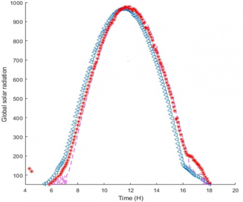
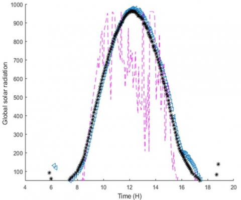
Figure 4 shows the performance of a selected HM, which provides the most accurate inclined GSR estimation, i.e., Bird and Hulstrom-Temps, and Bird & Hulstrom EM for an hourly solar profile of two different days in Bouzareah. Figure 4(a) portrays the estimation performance for a clear-sky day, May 15th, while Figure 4(b) presents the case of a cloudy-sky day, November 2nd. These figures demonstrate the accuracy of the selected HM for predicting the average behavior of the measured data curve compared to the EM for a solar profile.
(a)
(b)
Figure 4. Inclined GSR for (a) a clear sky day (15 May 2006) and (b) a cloudy sky day (02 November 2013)
This work investigates the performance of innovative HMs intended for estimating the 5-minute GSR on tilted surfaces for two locations in Algeria, Bouzareah and Ghardaia. These HMs are achieved by combining five EMs and five TMs, aiming mainly to improve the estimation accuracy of the semi-EMs in the case of overcast days. To demonstrate the effectiveness of the developed models, days in the dataset are classified based on sky conditions using a classification algorithm that relies on the clear index. The survey spanned twelve sample days throughout the year, beginning with assessments using only EMs, followed by HMs. The statistical results showed that the HMs yielded substantial enhancement over EMs, reducing NRMSE values by more than 90% in certain cases. For instance, the NRMSE value for the Bird & Hulstrom model on August 16th in Ghardaia was 25.07%. After integrating the Klucher model through hybridization, the NRMSE dropped to 5.32%. The proposed HMs demonstrated high accuracy even on overcast days, unlike standard EMs designed for clear skies. On December 10th, which was characterized by heavy cloud cover and a clearness index (KT) of 0.28, the Bird & Hulstrom EM alone yielded an NRMSE of 35%. But, when the Temps model was applied, the NRMSE decreased significantly to 13.37%. This analysis highlighted that the combinations of Bird & Hulstrom-Temps for Bouzareah and Bird & Hulstrom-Klucher for Ghardaïa provided the most accurate estimates on most days. Furthermore, it was also observed that integrating EMs with the Willmott transposition model was less effective. This research opened several avenues for future work, considering expanding the present study to cover additional regions and varying conditions, and examining the adaptability of the proposed approach to various temporal scales and horizons.
[1] Iqbal, M. (1983). Chapter 3 – The Solar Constant and its Spectral Distribution. In An Introduction to Solar Radiation, pp. 43-58. https://doi.org/10.1016/B978-0-12-373750-2.50008-2
[2] Jiang, W., Zhang, S., Wang, T., Zhang, Y., Sha, A., Xiao, J., Yuan, D. (2024). Evaluation method for the availability of solar energy resources in road areas before route corridor planning. Applied Energy, 356: 122260. https://doi.org/10.1016/j.apenergy.2023.122260
[3] Stambouli, A.B., Khiat, Z., Flazi, S., Kitamura, Y. (2012). A review on the renewable energy development in Algeria: Current perspective, energy scenario and sustainability issues. Renewable and Sustainable Energy Reviews, 16(7): 4445-4460. https://doi.org/10.1016/j.rser.2012.04.031
[4] Gueymard, C.A. (2001). Parameterized transmittance model for direct beam and circumsolar spectral irradiance. Solar Energy, 71: 325-346. https://doi.org/10.1016/S0038-092X(01)00054-8
[5] Alonso-Montesinos, J., Batlles, F.J., Bosch, J.L. (2015). Beam, diffuse and global solar irradiance estimation with satellite imagery. Energy Conversion and Management, 105: 1205-1212. https://doi.org/10.1016/j.enconman.2015.08.037
[6] Benatiallah, D., Zahouani, A., Yahiaoui, A., Djeldjli, H., Nasri, B., Benatiallah, A., Benabdelkrim, B. (2024). Estimating solar radiation based on machine learning approaches under Algerian desert climate. Instrumentation Mesure Métrologie, 23(5): 363-374. https://doi.org/10.18280/i2m.230504
[7] Tandon, A., Awasthi, A., Pattnayak, K.C., Tandon, A., Choudhury, T., Kotecha, K. (2025). Machine learning-driven solar irradiance prediction: Advancing renewable energy in Rajasthan. Discover Applied Sciences, 7: 107. https://doi.org/10.1007/s42452-025-06490-8
[8] Mujabar, S., Chintaginjala, V.R., (2021). Empirical models for estimating the global solar radiation of Jubail Industrial City, the Kingdom of Saudi Arabia. SN Applied Sciences, 3: 95. https://doi.org/10.1007/s42452-020-04043-9
[9] Sivakumar, M., Priya, S.J., Subathra, M.S.P. (2022). Global solar radiation prediction using empirical-based models. In 2022 International Conference on Applied Artificial Intelligence and Computing (ICAAIC), Salem, India, pp. 1635-1644. https://doi.org/10.1109/ICAAIC53929.2022.9793159
[10] Xiao, M., Yu, Z., Cui, Y. (2020). Evaluation and estimation of daily global solar radiation from the estimated direct and diffuse solar radiation. Theoretical and Applied Climatology, 140: 983-992. https://doi.org/10.1007/s00704-020-03140-4
[11] Hamdani, M., Bekkouche, S.M.A., Benouaz, T., Cherier, M.K. (2011). Etude et modélisation du potentiel solaire adéquat pour l’estimation des éclairements incidents à Ghardaïa. Revue Internationale d’Héliotechnique, 2(43): 8-13.
[12] S-Koussa, D., Koussa, M., Belhamel, M. (2006). Reconstitution du rayonnement solaire par ciel clair. Revue des Energies Renouvelables, 9(2): 91-97. https://doi.org/10.54966/jreen.v9i2.818
[13] Benkaciali, S., Gairaa, K. (2012). Comparative study of two models to estimate solar radiation on an inclined surface. Revue of Renewable Energies, 15(2): 219-228.
[14] Mesri-Merad, M., Rougab, I., Cheknaneand, A., Bachari, N.I. (2012). Estimation du rayonnement solaire au sol par des modèles semi-empiriques. Revue of Renewable Energies, 15(3): 451-463.
[15] Nia, M., Chegaar, M., Benatallah, M.F., Aillerie, M. (2013). Contribution to the quantification of solar radiation in Algeria. Energy Procedia, 36: 730-737. https://doi.org/10.1016/j.egypro.2013.07.085
[16] Bouramdane, A., Louazene, M.L., Benmir, A. (2023). Forecasting of inclined global solar radiation through empirical models applied in desert areas. In 4th International Conference on Technological Advances in Electrical Engineering (ICTAEE’23), Skikda.
[17] Lantri, F., Bachari, N.E.I., Belbachir, H. (2019). Estimating solar radiation in a clear sky on a horizontal surface from common meteorological data in Oran, Algeria. Revue of Renewable Energies, 22(1): 65-76. https://doi.org/10.54966/jreen.v22i1.726
[18] Soulouknga, M.C., Dandoussou, A., Djongyang, N. (2022). Empirical models for the evaluation of global solar radiation for the site of Abeche in the Province of Ouaddaï, in Chad. Smart Grid and Renewable Energy, 13: 223-234. https://doi.org/10.4236/sgre.2022.1310014
[19] Takilalte, A., Harrouni, S., Yaiche, M.R., Mora-López, L. (2020). New approach to estimate 5-min global solar irradiation data on tilted planes from horizontal measurement. Renewable Energy, 145: 2477-2488. https://doi.org/10.1016/j.renene.2019.07.165
[20] Dahmani, K., Dizene, R., Notton, G., Paoli, C., Voyant, C., Nivet, M.L. (2014). Estimation of 5-min time-step data of tilted solar global irradiation using an ANN (Artificial Neural Network) model. AIMS Energy, 70: 374-381. https://doi.org/10.1016/j.energy.2014.04.011
[21] Benatiallah, D., Benatiallah, A., Bouchouicha, K., Nasri, B. (2019). Estimation of clear sky global solar radiation in Algeria. AIMS Energy, 7(6): 710-727. https://doi.org/10.3934/energy.2019.6.710
[22] Van Heuklon, T.K. (1979). Estimating atmospheric ozone for solar radiation models. Solar Energy, 22(1): 63-68. https://doi.org/10.1016/0038-092X(79)90060-4