Vikram. M![]() | Sudhakar Uppalapati
| Sudhakar Uppalapati![]() | Ashok Battula
| Ashok Battula![]() | Srinivasa Babu Kasturi
| Srinivasa Babu Kasturi![]() | Harinadh Vemanaboina
| Harinadh Vemanaboina![]() | Satish Kumar*
| Satish Kumar*![]()
© 2025 The authors. This article is published by IIETA and is licensed under the CC BY 4.0 license (http://creativecommons.org/licenses/by/4.0/).
OPEN ACCESS
This study was used to predict the process parameters for control of residual stress for laser welding of stainless-steel plates using random forest algorithms in Machine Learning techniques. The model's inputs were laser power, welding speed, and shielding gas, and the resulting response was residual stress. The random forest algorithms are trained with 70% input data and 30% correlation for the targeted output. MATLAB was used initially for training using the random forest technique, the root means square error (RMSE), an absolute fraction of variance (R2), and mean absolute percentage error (MAPE) was carried out, and Python codes were used to predict the best combinations. According to the Python code, the laser power is predicted to be 3.25 kW, the welding speed is 2.45 mm/min, and the shielding is 15 LPM. The validation was carried out using FEA for thermal analysis to verify the weldability temperature, which was found to be 2310oK, and the final residual stresses were verified with the existing literature. The predicted process parameters are suitable for SS to have minimal residual stresses.
laser welding, machine learning, random forest, residual stress, FEA
Machine learning, a branch of artificial intelligence, allows computers to learn and develop independently via practical knowledge. It has attained prominence across several domains, including information technology, data security, robotics, manufacturing, and others [1, 2]. As more individuals get acquainted with the concept, its popularity and utilization expand [3, 4]. The ability to replicate human intelligence and learning provides a significant advantage over conventional approaches to doing identical tasks. Laser welding uses ML methods for precision, simplicity of implementation, and generalizability across all manufacturing procedures. AI methods optimize and estimate many parameters to attain high quality, low residual, and distortion in laser welding [5]. Numerous factors, including laser intensity, laser velocity, and gas movement, affect the quality of a laser weld. This set of variables is interconnected but operates separately. Laser welding relies heavily on artificial intelligence methods, notably the random forest algorithm. These methods foretell the outcomes of laser welding processes, such as generating residual stress and distortion-free weld connections. The primary users of the laser welding technique are established manufacturing plants in the aviation, aerospace, and automotive sectors. The laser beam welding business uses lasers for speed, accuracy, and power, but some drawbacks exist [6]. Laser-welded metals like high-carbon steels crack due to fast cooling [7]. Steel, aluminum, and titanium are suitable for laser beam welding.
Residual stresses remain in a material after the original source of the stress has been removed. In welding, uneven heating and cooling cycles often induce these stresses. The intense localised heat generated during welding causes the material in the weld zone to expand [8]. Upon cooling, it undergoes contraction; however, this shrinkage is constrained by the adjacent cooler material, leading to plastic deformation and tensile and compressive stresses inside the welded joint and heat-affected zone (HAZ). The material experiences temperature differences throughout its whole due to rapid thermal cycling [9]. Changes in materials like steel, such as the transition of austenite to martensite, may also alter volumetric properties. Internal stresses are produced due to the inflexible material surrounding the weld, which restricts the weld's ability to expand and contract without restriction. During the process of the molten weld pool becoming more solid, shrinkage occurs, which leads to tensile stresses. It is possible that cold cracking or delayed hydrogen-induced cracking might be facilitated by elevated tensile residual stress. This is because residual stresses reduce the fatigue resistance of joints that have been welded [10]. The residual stresses may significantly affect weld quality by increasing the risk of distortion, reducing the fatigue life of the weld, and leading to stress corrosion cracking or brittle fracture. To ensure the structural integrity and performance of welded components, it is essential to comprehend these stresses and exert control over them.
In the material processing industry, materials must be treated with precision and consistency to meet the required quality requirements. Consequently, lately, a neural network has been used to process linked components called neurons. Utilizing a computer, machine learning may autonomously discern all established physical laws, provided it is equipped with enough data and techniques. By analyzing a data segment, the machine learning methodology may discern underlying principles and autonomously develop a predictive model [11-13].
Cutting an opening in the object dramatically enhances the quality of the laser stream that reaches the material being worked. Moving the joint relative to the laser beam or the opening along the joint to be formed allows for full penetration in the welding. This method results in rivets with greater penetration than bead width. Under vapour pressure and surface tension, the liquid material at the keyhole's leading edge moves around the beam hollow to the rear and hardens to make the weld. Beads at the top of the joint with a zigzag design indicate where the welding process started. Compressive bending around the liquid zone causes leftover stress as the material warms and swells during welding. As the joint metal cools and shrinks, a tensile residual tension is produced, especially along the lengthwise axis [14]. Compressive stress develops at greater distances from the weld zone to counteract the leftover tensile stress that persists across the joint center line after welding [15]. The tension and excess stress on the weld line and any gaps or flaws connected with the weld bead decrease endurance, strength, and durability. The lengthwise residual stress in the seam and area is high tensile, while the top tube is compressive. The weld's crosswise residual stress is low tensile stress near the top surface and compressive stress near the bottom [16].
The structure deforms, resulting in distortion, to improve some of the residual stress brought on by the welding process. Buckling distortion, caused by compressive stress in the base material, is the primary distortion, especially in thin welded structures. Buckling distortion may also arise from other types of distortion. There are several distortion modes, but buckling distortion is the most common. New high-strength materials that make it possible to use thinner sections with fewer critical buckling loads increase the likelihood of buckling distortion [17]. Artificial intelligence (AI) is the focal point of technological advancements, benefiting both people and companies. Optical character recognition (OCR) extracts text and data from images and documents using artificial intelligence. This method transforms raw resources into actionable knowledge for companies [18-20]. Artificial intelligence is a field focused on creating computers and robots capable of thinking, learning, and doing activities that typically require human intellect or involve data sets too vast for human analysis.
Metals and alloys have been studied extensively, but most are isotropic materials with uniform thermal conductivity along horizontal lines. Materials exhibiting anisotropic thermo-physical properties and cold-rolled hard solids are used in nuclear power plants because of the intrinsic variance in thermal energy transfer across many orthogonal directions. Nuclear power plants are designed to accommodate this natural variability. Compared to isotropic materials, there is far less available literature on these materials. Uneven heat transfer through these materials increases thermal stress and leads to distorted end products. Therefore, a detailed heat transfer analysis in orthotropic substances is needed to forecast the thermal field and develop an appropriate cooling strategy.
This study's results illustrate that various welding processes may benefit from machine learning techniques, significantly improving efficiency and accuracy. Machine learning has been used to address challenges like quality monitoring, talent needs, time consumption, and others. The available literature is limited in predicting residual stress using Machine learning techniques of Stainless steel in laser joints. The controllable process parameters are used to train the algorithm using the data from the available literature. The ANN tool with the Random Forest Regression Machine Learning Algorithm was used in this analysis. A range of statistical indicators pertains to this domain. Indicators include the root mean square error (RMSE), the coefficient of determination (R²), the mean absolute percentage error (MAPE), the ability of methods to generalize across test and training datasets, and residual plots as a function of specific input parameters. The predicted process parameters for residual stress are discussed. ANSYS is used for thermal analysis using a Gaussian heat source to confirm the predicted parameters regarding weldability.
Sharper laser beams may increase thermal input and penetration depth, leading to stronger thermal gradients and more residual stress. The laser intensity must be fine-tuned to achieve sufficient penetration with minimal heat production. Accelerated welding reduces the HAZ size and residual stress by shortening the time for the heat cycle to complete. The converse is also true: fusion quality could be compromised quickly, resulting in flaws. Weld quality may be assured to meet demanding industrial requirements using advanced control systems and intelligent algorithms, which can increase accuracy and consistency. To optimise parameter optimisation, machine learning methods may establish a correlation between process parameters and residual stress results.
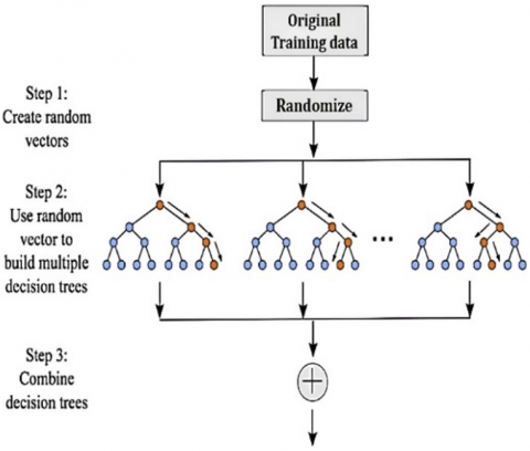
The random forest algorithm may resolve classification and regression problems in machine learning, as seen in Figure 1. We all know that a forest is only as mighty as its trees and that there must be many trees to be considered a forest. The precision and problem-solving effectiveness of a Random Forest method are directly proportional to the number of trees used in method [21]. Random Forest classifiers use the sum of several decision trees on different dataset groups to improve forecast accuracy. It relies on the concept of ensemble learning, in which numerous classifications are pooled together to improve the performance of a model for a challenging task [22].
(a)
(b)
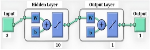
Figure 1. (a) Random forest algorithm (b) Neural network
The random forest algorithm has several benefits. The main advantages are a decreased risk of overfitting and a decrease in the time required for training. Furthermore, it offers a significant degree of accuracy as well. The RF method handles large data sets rapidly by inputting missing data, leading to exact predictions. This is done to provide predictions. The random forest algorithm is explained in the following steps:
Step 1: Select irregular examples from a given information or preparation set.
Step 2: Utilising this strategy, a decision tree will be constructed for each training dataset.
Step 3: The decision tree will be averaged as the voting process progresses.
Step 4: Select the predicted result that received the most votes.
The parameter settings used for the random forest algorithm are the number of trees set to 100 and the maximum depth of each tree limited to 10. These values were chosen based on preliminary experimentation and cross-validation to balance model accuracy with computational efficiency and prevent overfitting. A grid search was also conducted to tune these hyperparameters, evaluating combinations of tree counts as 100 and depth limits as 10. The selected settings yielded the best performance on validation data regarding accuracy and generalization.
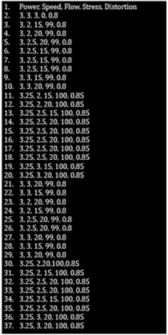
Table 1 shows the input parameters for laser welding: laser power, speed, and gas flow rate. These parameters and the responses were primarily obtained from simulations and experimental data collected during our welding trials under controlled laboratory conditions from literature as given in Table 1. The program uses these parameter values to predict the best values. Figure 2 shows the neural network structure for the given inputs. By training the inputs, an ANN network can be generated so that we can declare how many layers are needed to train the data. It mainly separates the hidden layer and output layers. The above network takes 3 inputs and fixed with 1 response. The single hidden layer backpropagation neural networks (BPNNs) in Figure 1(b) used in this study have one neuron for residual stress and three nodes in the input layer representing laser power, speed, and flow rate, respectively. During the training, the number of hidden layer neurons was considered a variable parameter and ranged from 5 to 15. The hidden and output layer neurons' respective activation functions are considered sigmoidal and linear, respectively.
Table 1. Inputs for the program [8-11, 14, 16]
|
Laser Power |
Laser Speed |
Argon Flow Rate |
Residual Stresses |
|
kW |
m/min |
LPM |
MPa |
|
3.0 |
2.0 |
15 |
100 |
|
3.0 |
2.0 |
15 |
109 |
|
3.0 |
2.0 |
20 |
70 |
|
3.0 |
2.5 |
15 |
78 |
|
3.0 |
2.5 |
15 |
88 |
|
3.0 |
2.5 |
20 |
99 |
|
3.0 |
3.0 |
15 |
68 |
|
3.0 |
3.0 |
20 |
76 |
|
3.0 |
3.0 |
15 |
107 |
|
3.5 |
2.0 |
20 |
98 |
|
3.5 |
2.0 |
15 |
96 |
|
3.5 |
2.0 |
20 |
95 |
|
3.5 |
2.5 |
15 |
101 |
|
3.5 |
2.5 |
20 |
116 |
|
3.5 |
2.5 |
15 |
101 |
|
3.5 |
2.5 |
15 |
112 |
2.1 Application of random forest algorithm using Python code
Regression and classification are two tasks that may be accomplished using the Random Forest ensemble learning approach. It produces several decision trees and consolidates their outcomes to improve forecast accuracy and reduce the likelihood of overfitting. Here are the detailed steps for the random forest algorithm:
Data transformation includes scaling, normalizing, and encoding the data to ensure it is in the proper format for the random forest method.
Feature selection involves selecting the most relevant features from the input data to improve performance and reduce the complexity of the random forest model.
Splitting the input data into a training set and a test set allows us to train the random forest model on one set of data and evaluate its performance on the other. By following these procedures for data preparation, you may train the random forest model on high-quality data, allowing for accurate predictions.
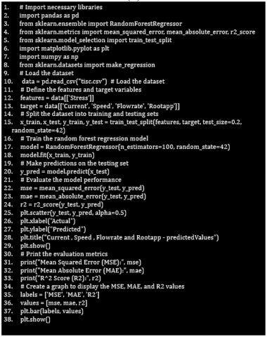
Step 2 is to prepare a Python program to train the data as shown in Figures 2 (a) and (b). We import the iris dataset into the training and testing subsets using the train-test split tool. This is accomplished by using the input data as the source data. Subsequently, we construct a Random Forest classifier object designated as RF, with 42 trees. Thereafter, we use the fit function to calibrate the model using the training data, subsequently applying the prediction method to forecast results on the test data. We evaluate the classifier's performance utilizing the accuracy score function from scikit-learn. In conclusion, we determine that the classifier is efficient.
Figures 2 (a) and (b) show the program for random forest algorithm where in the first python program it created for the residual stress with 100 neurons where the set of input data that is laser power laser speed, and gas flow rate are imported according to this the fix the target value that is 100 N/mm2. This Python program can also include the program for graph generation that graphs mean square error, mean absolute error, and R2 value.
(a)
(b)
Figure 2. Python programing (a) Import input data into algorithm (b) Program for residual stress
The model was developed using Python 3.9, and the following libraries were utilized with their respective versions:
Additionally, the key functions and steps involved in the process have been clearly described, train_test_split for splitting the dataset (80% training, 20% testing).
2.2 Finite element analysis
The Gaussian distribution heat source model simulates the transient thermal analysis with parameter inputs as predicted from the Random Forest techniques presented in section 3. The 3D model plate uses ANSYS with 100 mm×100 mm×5 mm dimensions. A solid 70 elements are used, an 8-node structure with one degree of freedom per node. Three different meshing methods are used: 1mm at the weld, 2mm at the HAZ, and 8 mm throughout the plate. The SS316 temperature-dependent properties were used for simulation.
2.2.1 Boundary conditions
2.3 Governing equation
Eq. (1) governs welding using a laser beam at 1.5 m/min speeds, which shows three-dimensional heat conduction.
$c \rho \frac{\partial^2 T}{\partial X^2}=k\left(\frac{\partial^2 T}{\partial X^2}\right)+k\left(\frac{\partial^2 T}{\partial Y^2}\right)+k\left(\frac{\partial^2 T}{\partial Z^2}\right)+Q$ (1)
$H=24.1^* 10^{-4} \varepsilon T^{1.61}$ (2)
The combined heat emission and diffusion coefficients from the welded material's top surface yield the following Eq. (2).
$\mathrm{q}(\mathrm{r})=\mathrm{q}(0) \mathrm{e}^{-\mathrm{c}^2}$ (3)
Eq. (3) specifies the flow distribution across the Gaussian surface, with the heat flux at a specific distance r from the heat source as 2mm, and C is constant.
Random forest is a well-liked classification and regression algorithm. Because classification and regression are the most crucial aspects of the field, the random forest algorithm shown in Figure 3 is one of the most significant algorithms in machine learning. Correctly classifying observations benefits various applications, such as prediction and optimization. The random forest algorithm can predict the laser power, speed, and gas flow rate for the laser welding process parameters. The residual stresses of the laser welding output can also be predicted using this algorithm [23]. This can be accomplished by creating a set of inputs in an Excel sheet, copying them, and importing them into a random forest algorithm program. After running the imported program, we obtained outputs with a lower mean square error suitable for the laser welding procedure. The Random Forest method is a supervised machine-learning technique that integrates the predictions of many algorithms [24-26]. Random Forest uses the ensemble learning technique to predict the output variables rather than the ensemble learning approach [27, 28]. As a result, it produces output predictions that are more accurate than those made by a single model [29-31].
(a)
(b)
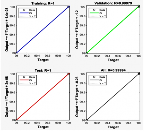
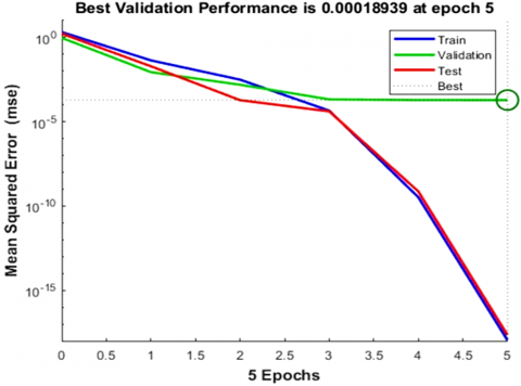
Figure 3. Matlab was used for (a) The regression performance of the developed model. (b) Network performance on datasets
The total size of the input and output data sets was a matrix of 3 by 18 and 1 by 18. The neural network received 80% of the input data for model training, while the testing and validation phases of the ANN model development each received 20% of the input data. A model with an R-value (correlation value) of 1.0 for training data, an R-value (correlation value) of 0.9997 for validation data, an R-value (correlation value) of 1.0 for test data, and finally, an R-value (correlation value) of 0.9999 for an overall correlation between the actual outputs and the targets were obtained after several training iterations.
Table 1 shows the predicted process parameters for the respected targets, i.e., laser power, speed, and gas flow rate. Residual stress is fixed to 99 and 100 N/mm2. The above process parameters meet the requirements for training the given data. It provides the regression of the R-value near 1, so we can reduce the residual stresses with the help of these predicted values.
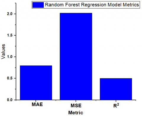
Figure 4 shows the results of the random forest algorithm for residual stress. It indicates that the MAE, MSE, and R2 values, where MAE is 0.89 and MSE is 2.02, are always more than MAE, and the R2 value is 0.58. These values are always less than 1 or equal to 1. MAE measures the average absolute difference between the predicted and actual values. A value around 0.9 suggests that, on average, the model's predictions deviate from the actual values by 0.89 units. This indicates moderate accuracy, depending on the scale of the output variable. Lower MAE values are desirable. This MAE indicates reasonably good performance, but there's room for improvement. MSE squares the error before averaging, giving higher weight to more significant errors. A value around 2.02 implies that some predictions have higher variance from actual values. R² indicates the proportion of variance in the target variable explained by the model. This relatively high MSE compared to MAE suggests the model may produce occasional significant errors. Outliers might be influencing this. A value of 0.58 suggests that the model explains 58% of the variance, which reflects limited explanatory power. The model has captured some patterns in the data but may benefit from additional features.
Figure 4. Regression graph for MSE, MAE, R2 values of residual stresses
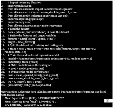
Figure 5. Trained program for residual stress
Figure 5 shows the program for residual stress; we input the given data and train the program, then input the data set into the program and train it to get the output. Figure 4 depicts the laser welding process, outlining the expected operational parameters. The variables include the laser's power, speed, and gas flow rate. All these distinctive characteristics are shown at various phases of the data-collecting process. Alongside the R², MSE and MAE are all shown; these three terms can decide whether the predicted values are absolute. When the R2 is always less than 1, the MSE is less than 10, and the final MAE is less than the MSE. In this condition, only the predicted values are perfect. From Figure 5, the program shows that fixing 100 N/mm2 stress gives 3.25 kW, 2.5 mm/sec, and 17.19 LPM of laser power, laser speed, and gas flow rate, respectively. The R2 value is 0.58, the MSE is 2.02, and the MAE is 0.8, so all aspects are within the condition, and the predicted process parameters for residual stress are accurate.
3.1 Validation through FEA and existing literature
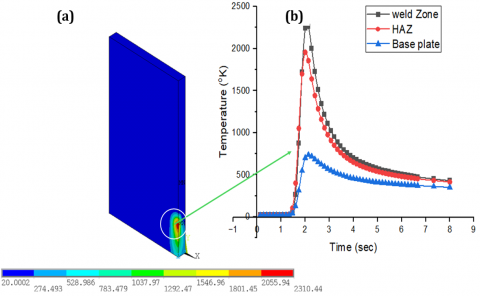
The investigation revealed significant variations in temperature throughout the length of the plate, which may be attributed to its elevated thermal conductivity. In the fusion zone, temperatures peaked due to the high energy contraction at the weld during the experiment. Radiation from the fusion zone was distributed throughout the weld as it generated heat. In Figure 6, weld temperatures are measured at the top of the weldment to show the temperature distribution of the welds. Temperature distribution during welding is recorded at the start of the welding process and before the weld plate. In Figure 6(a), the temperature at the starting is 2310oK at 2sec after the beginning of the weld (with 3.25kW and speed 1.5mm/min), and Figure 6(b) illustrates the temperature distribution in the transverse direction at 2 seconds and the melting temperature of stainless steel is 1700oK.
Figure 6. Temperature distribution at 2 sec of time
The temperature has risen to the extent that the base material is beginning to boil (the melting point of SS is 1700 °K), resulting in the expansion of the keyhole due to evaporation. A material's melting point is the temperature at which it attains its maximum state above the solidus temperature [32]. Should the temperature be above the liquidus temperature, total melting will occur. The temperature exhibits symmetry due to the uniform geometry distribution, heat flow, and boundary conditions.
The temperature is above the melting point, which needs confirmation through experimentation. From the available literature for stainless steel, the welding temperature reaches 1700 °K, and the residual stresses vary from 20 MPa to 178 MPa (both tensile and compressive in nature based on the boundary conditions), which requires experimental validation. It also confirms that the factor of safety is above 1.0, as required for stainless steel. The selection of production parameters in the laser welding process, which is recognised as an innovative manufacturing method, is frequently based on employee experience. This can have some adverse effects, including increased production costs, ineffective products, and lost time.
Selecting the production parameters in the laser welding process is an innovative and inventive manufacturing method. Recent advancements in machine learning techniques have enabled the selection of input parameters and the prediction of output parameters for laser welding with enhanced accuracy. This paper has thoroughly examined and evaluated standard ML methods for laser welding.
•The most frequently used artificial intelligence method, with an accuracy rate of approximately 99%, was found to be ANN in studies. Nevertheless, artificial neural network prediction studies are highly accurate.
•The predicted critical process parameters are a laser power of 3.25 kW, a welding speed of 2.5 m/sec, and shielding gas of 17 LPM for residual stress below 100 N/mm2, as well as the prediction from ANN and Random Forest method algorithms.
•The prediction of laser welding quality was complex due to many factors.
•FEA is used to simulate the process in the first phase to confirm the weldability of plates with the predicted parameters; the temperature is above the melting temperature of the base material.
Integrating Machine learning algorithms is best suited for predicting process parameters for more accuracy for the fixed targets to minimize the residual stresses or other responses.
|
CP |
specific heat, J. kg-1. K-1 |
|
k |
thermal conductivity, W.m-1. K-1 |
|
hr |
radiation boundary condition |
|
Q |
net heat, W.m3 |
|
C |
constant |
|
Greek symbols |
|
|
a |
thermal diffusivity, m2. s-1 |
|
ρ |
density, kg/m3 |
|
ε |
emissivity of surface radiating |
[1] Rodrigues, M., Kormann, M., Schuhler, C., Tomek, P. (2013). An intelligent real time 3D vision system for robotic welding tasks. In 2013 9th International Symposium on Mechatronics and Its Applications (ISMA), Amman, Jordan, pp. 1-6. https://doi.org/10.1109/ISMA.2013.6547393
[2] Chen, C., Lv, N., Chen, S. (2018). Data-driven welding expert system structure based on internet of things. In Transactions on Intelligent Welding Manufacturing, Springer Singapore, pp. 45-60. https://doi.org/10.1007/978-981-10-8330-3_3
[3] Wang, B., Hu, S.J., Sun, L., Freiheit, T. (2020). Intelligent welding system technologies: State-of-the-art review and perspectives. Journal of Manufacturing Systems, 56: 373-391. https://doi.org/10.1016/j.jmsy.2020.06.020
[4] Yifei, T., Meng, Z., Jingwei, L., Dongbo, L., Yulin, W. (2018). Research on intelligent welding robot path optimization based on GA and PSO algorithms. IEEE Access, 6: 65397-65404. https://doi.org/10.1109/ACCESS.2018.2878615
[5] You, D.Y., Gao, X.D., Katayama, S. (2014). Review of laser welding monitoring. Science and Technology of Welding and Joining, 19(3): 181-201. https://doi.org/10.1179/1362171813y.0000000180
[6] Kucukoglu, A., Yuce, C., Sozer, I.E., Karpat, F. (2023). Multi-response optimization for laser transmission welding of PMMA to ABS using Taguchi-based TOPSIS method. Advances in Mechanical Engineering, 15(8): 16878132231193260. https://doi.org/10.1177/16878132231193260
[7] Phanikumar, G., Dutta, P., Chattopadhyay, K. (2005). Continuous welding of Cu–Ni dissimilar couple using CO2 laser. Science and Technology of Welding and Joining, 10(2): 158-166. https://doi.org/10.1179/174329305x36043
[8] Arroju, P., Panchagnula, K.K., Saritha, P., Nune, M.M.R., Madhura, K., Kumar, J.S., Vemanaboina, H., Naidu, G.G. (2023). Analysis of residual stress in SS321 laser butt-welded plates using finite element analysis. International Journal on Interactive Design and Manufacturing (IJIDeM), 18(5): 2897-2902. https://doi.org/10.1007/s12008-023-01362-0
[9] Yelamasetti, B., Ramana, G.V., Manikyam, S., Vardhan T, V. (2022). Thermal field and residual stress analyses of similar and dissimilar weldments joined by constant and pulsed current TIG welding techniques. Advances in Materials and Processing Technologies, 8(sup3): 1889-1904. https://doi.org/10.1080/2374068X.2021.1959114
[10] Yelamasetti, B., Panchagnula, J.S., Padamurthy, A., Vemanaboina, H., Prakash, C., Paramasivam, P. (2024). Microstructure and mechanical analysis of SS321 in CO2 laser beam welding joint. The International Journal of Advanced Manufacturing Technology, 135(11): 5861-5874. https://doi.org/10.1007/s00170-024-14850-8
[11] Balasubramanian, K.R., Buvanashekaran, G., Sankaranarayanasamy, K. (2010). Modeling of laser beam welding of stainless steel sheet butt joint using neural networks. CIRP Journal of Manufacturing Science and Technology, 3(1): 80-84. https://doi.org/10.1016/j.cirpj.2010.07.001
[12] Liu, B., Jin, W., Lu, A., Liu, K., Wang, C., Mi, G. (2020). Optimal design for dual laser beam butt welding process parameter using artificial neural networks and genetic algorithm for SUS316L austenitic stainless steel. Optics & Laser Technology, 125: 106027. https://doi.org/10.1016/j.optlastec.2019.106027
[13] Olanipekun, A.T., Mashinini, P.M., Owojaiye, O.A., Maledi, N.B. (2022). Applying a neural network-based machine learning to laser-welded spark plasma sintered steel: Predicting Vickers micro-hardness. Journal of Manufacturing and Materials Processing, 6(5): 91. https://doi.org/10.3390/jmmp6050091
[14] Mohanty, S., Arivarasu, M., Arivazhagan, N., Phani Prabhakar, K.V. (2017). The residual stress distribution of CO2 laser beam welded AISI 316 austenitic stainless steel and the effect of vibratory stress relief. Materials Science and Engineering: A, 703: 227-235. https://doi.org/10.1016/j.msea.2017.07.066
[15] Goldak, J., Chakravarti, A., Bibby, M. (1984). A new finite element model for welding heat sources. Metallurgical Transactions B, 15(2): 299-305. https://doi.org/10.1007/bf02667333
[16] Vemanaboina, H., Purushotham, A., Reddy, K.S., Reddy, P.N., Prakash, C., Kumar, R., Mehdi, H. (2024). Optimization of process parameters of CO2 laser beam butt joints of SS321. International Journal on Interactive Design and Manufacturing (IJIDeM), 2024: 1-13. https://doi.org/10.1007/s12008-024-02095-4
[17] Parks, R.W., Levine, D.S., Long, D.L. (1998). Fundamentals of neural network modeling: Neuropsychology and cognitive neuroscience. Mit Press. https://doi.org/10.7551/mitpress/3163.003.0005
[18] Gardner, D. (1993). Introduction: Toward neural neural networks. Mit Press, pp. 1-12. https://doi.org/10.7551/mitpress/4941.003.0004
[19] Bernacki, A. (2024). Modern methods and algorithms of path planning for autonomous mobile robots, their objective functions. Communication, Informatization and Cybersecurity Systems and Technologies, 1(6): 24-58. https://doi.org/10.58254/viti.6.2024.02.24
[20] Mukhopadhyay, S., Kumar, A., Gupta, J., Bhatnagar, A., Kantipudi, M.P., Singh, M. (2024). A review and analysis of IoT enabled smart transportation using machine learning techniques. International Journal of Transport Development and Integration, 8(1): 61-77. https://doi.org/10.18280/ijtdi.080106
[21] Chen, X., Güttel, S. (2024). Fast and exact fixed-radius neighbor search based on sorting. PeerJ Computer Science, 10: e1929. https://doi.org/10.7717/peerj-cs.1929/table-6
[22] Bock, F.E., Blaga, L.A., Klusemann, B. (2020). Mechanical performance prediction for friction riveting joints of dissimilar materials via machine learning. Procedia Manufacturing, 47: 615-622. https://doi.org/10.1016/j.promfg.2020.04.189
[23] Kantipudi, M.P., Vemuri, S., Sreenath Kashyap, S., Aluvalu, R., Satish Kumar, Y. (2020). Modeling of microstrip patch antenna using artificial neural network algorithms. In International Conference on Advanced Informatics for Computing Research, Singapore: Springer Singapore, pp. 27-36. https://doi.org/10.1007/978-981-16-3653-0_3
[24] Kantipudi, M.P., Kumar, S., Kumar Jha, A. (2021). Scene text recognition based on bidirectional LSTM and deep neural network. Computational Intelligence and Neuroscience, 2021(1): 2676780. https://doi.org/10.1155/2021/2676780
[25] Sani, V., Kantipudi, M.V.V., Meduri, P. (2023). Enhanced SSD algorithm-based object detection and depth estimation for autonomous vehicle navigation. International Journal of Transport Development and Integration, 7(4): 341-351. https://doi.org/10.18280/ijtdi.070408
[26] NS, P.K., Kantipudi, M.P., N, P., S, S., Aluvalu, R., Jagtap, J. (2024). A security analysis model for IoT-ecosystem using machine learning-(ML) approach. Recent Advances in Computer Science and Communications (Formerly: Recent Patents on Computer Science), 17(6): 39-47. https://doi.org/10.2174/0126662558286885240223093414
[27] Buchade, A.C., Kantipudi, M.P. (2024). Recent trends on brain Tumor detection using hybrid deep learning methods. Revue d'Intelligence Artificielle, 38(1): 103-113. https://doi.org/10.18280/ria.380111
[28] Babaiyan, V., Mollayi, N., Taheri, M., Azargoman, M. (2022). An ensemble random forest model to predict bead geometry in GMAW process. Journal of Advanced Manufacturing Systems, 21(2): 393-410. https://doi.org/10.1142/s021968672250007x
[29] Çavuşoğlu, Ü. (2019). A new hybrid approach for intrusion detection using machine learning methods. Applied Intelligence, 49(7): 2735-2761. https://doi.org/10.1007/s10489-018-01408-x
[30] Gopal, P.M., Kavimani, V., Sudhagar, S., Barik, D., Paramasivam, P., Vemanaboina, H. (2024). Enhancing WEDM performance on Mg/FeCoCrNiMn HEA composites through ANN and entropy integrated COCOSO optimization. AIP Advances, 14(9): 095213. https://doi.org/10.1063/5.0226558
[31] Piekarska, W., Kubiak, M. (2012). Theoretical investigations into heat transfer in laser-welded steel sheets. Journal of Thermal Analysis and Calorimetry, 110(1): 159-166. https://doi.org/10.1007/s10973-012-2486-0
[32] Vemanaboina, H., Kunduru, K.R., Kumar, P.K., Goud, R.R., Gowd, G.H. (2024). Mechanical properties of CO2 laser beam butt-welded plates of Hastelloy c-276. Proceedings of the Institution of Mechanical Engineers, Part E: Journal of Process Mechanical Engineering, 2024: 09544089241239620. https://doi.org/10.1177/09544089241239620