Sana Khalid Abdulhassan*![]() | Mouna Ben Smida
| Mouna Ben Smida![]() | Anis Sakly
| Anis Sakly![]() | Firas Mohammed Tuaimah
| Firas Mohammed Tuaimah![]()
© 2025 The authors. This article is published by IIETA and is licensed under the CC BY 4.0 license (http://creativecommons.org/licenses/by/4.0/).
OPEN ACCESS
Power transmission networks play a critical role in linking generation and distribution systems. One key aspect of the network's performance is voltage optimization. This study focuses on comparing the impacts of High-Voltage Direct Current (HVDC) transmission and Flexible Alternating Current Transmission Systems (FACTS), specifically the Unified Power Flow Controller (UPFC), on system voltage stability, grid power losses, and transmission capacity under load fault conditions. This present study develops the IEEE 30-bus and IEEE 57-bus systems as test cases, incorporating Genetic Algorithms (GA) to analyze the effects of HVDC and UPFC integration. The Power System Simulator for Engineering (PSS/E) version 33 software program is used to model multi-terminal UPFC and HVDC. A comparative study is performed between the system's performance with and without HVDC and UPFC under various load conditions in the transmission network. Three load conditions were analyzed. The results demonstrate that for the IEEE 30-bus system, the total active power loss under normal load conditions is reduced by 69.594% after adding UPFC between buses (3-4) and by 75% after introducing multi-terminal VSC-HVDC between buses (2-6) and (2-4). Similarly, reactive power losses are reduced by 74% with UPFC and 73% with multi-terminal VSC-HVDC under the same conditions. For the IEEE 57-bus system, the addition of UPFC and VSC-HVDC improves active and reactive power losses by 49% and 55%, respectively, under normal load conditions. The studied results confirm that connecting HVDC to the system achieves better results in terms of bus voltage profile, a significant reduction in total network power losses, and a higher effective power transfer rate compared to UPFC. Moreover, multi-terminal HVDC transmission delivers greater voltage improvements and larger reductions in total power losses compared to adding UPFC to the same system.
multi terminal VSC-HVDC, UPFC, power flow control, MATLAB, PSS/E, active power, reactive power, IEEE-30, IEEE-57
The increase in demand in our daily life is one of the important things that must be taken into consideration because it requires an increase in the rate of electrical energy, because this exposes electrical power transmission networks to operate under high pressures and unstable voltages [1]. Therefore, it is important to develop electrical transmission networks in terms of control and equipping networks with devices that increase the rate of energy supply to confront these complexities and the increase in demand rate [2]. Whereas the FACTs and technologies of high-voltage direct current (HVDC) transmission have many advantages such as they can be used to control power flow, transmit maximum power, control voltage, compensate reactive power, improve stability and power quality and power conditioning [3].
A very powerful FACTS tool for managing power flow, lowering transmission losses, improving stability, and increasing transmission efficiency is the (UPFC) control system. However, obstacles to its wider implementation include its high cost, complexity, and maintenance needs. Notwithstanding these drawbacks, this system is still an essential piece of technology for contemporary power grids, especially when it comes to integrating renewable energy sources and improving system dependability.
With features like grid connectivity, long-distance efficiency, and integration of renewable energy, HVDC is a crucial component of contemporary power systems. However, its broad adoption is constrained by high costs, complexity, and compatibility problems. HVDC is anticipated to become more prevalent in energy systems of the future due to developments in multi-terminal networks and VSC-HVDC [4, 5].
Unified Power Flow Controller (UPFC) which can be defined as a versatile device characterized by high flexibility, reliability and flexibility through which the flow of real and reactive power can be controlled and the independent control of voltage and redistribution of power in a way that can be used to exploit areas with low load to peak areas in transmission lines [6].
In the other hand, transmitting power over long distances and through asynchronous systems requires the use of high-voltage direct current (HVDC) to be considered useful and effective for this purpose. High-voltage direct current cables and lines compared to three-phase alternating current transmission lines are less expensive, have fewer losses and require fewer transmission lines High-voltage direct current connections offer steady capacity without being constrained by network congestion or loop flow on parallel paths since they are controllable [7, 8]. The large power can be transmitted without distance conditions through high-voltage direct current cable systems that use fewer cables than alternating current cable systems due to their charging current. VSC-HVDC provides the network with high control methods for both active and reactive power independently of each other [9].
To achieve the best results that improve network functionality, this requires good selection of the optimal location and the best size for both MT-HVDC and UPFC components [10, 11]. After the loaded transmission lines in the system are identified, Genetic Algorithm (GA) will be used to locate the optimal HVDC and UPFC power systems under the normal system load capacity with safely operation. GA supports the search for optimal placement, best generation and optimal size of the UPFC and HVDC to maintain the voltage system profile, minimize the total active and reactive power losses. Where the UPFC and HVDC parameter rate and control the power flow in the overloaded transmission lines [12].
In reference [13], the optimal location of FACTS devices that is UPFC and HVDC are investigated using Power Flow Analysis in order to decrease the active power losses which analyzed on WSCC 3 machine 9 bus system and its doing using PSAT (Power System Analysis Toolbox) software. While in study [14], the study examined the advantages of using high voltage DC and FACTS devices in power systems such as increased power transmission capacity, improved static and dynamic stability, increased availability and reduced transmission losses using power electronics technologies. In the study [15], the comparison of the performance of HVDC transmission and UPFC controller, the controllers can work with multiple operating modes to control voltage, active power, reactive power flow and transmission line. The obtained results demonstrate the feasibility of the proposed models in solving Newton-Raphson power flow. These devices can be used by a company that can implement HVDC transmission with multiple control function and also UPFC with the following control types [16, 17].
The Power System Simulator for Engineering (PSS/E) is one of the programs used to analyze and design electrical networks in a smooth, flexible and highly reliable manner in identifying problems to be addressed. As a result, PSS/E has been widely utilized to analyze electrical networks. Additionally, real power system data can be used with PSS/E to show how the HVAC and UPFC power grids interact with the HVDC power grid [18, 19].
2.1 UPFC system model
The concept of The Unified Power Flow Controller, or UPFC, is a power electronics-based system that allows for the simultaneous management of active and reactive power flow rate, phase angle, transmission line issues, and voltage magnitude [20]. UPFC have two voltage source convertors: one acts as shunt converter called a STATCOM and the other series converter called a SSSC. In series with the line, the SSSC converter regulates the phasor voltage. Through this voltage source, the transmission line current exchanges active and reactive power with the AC system [21]. Additionally, the transformer that connects the STATCOM converter to the power supply allows it to exchange reactive power with the system. A DC capacitor serves as the connection between STATCOM and SSSC [22].
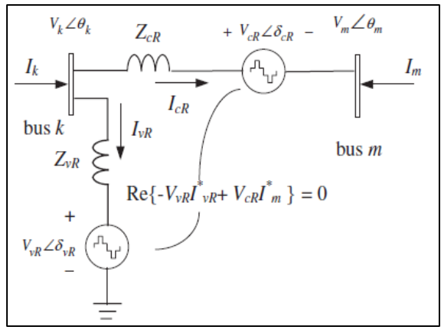
The STATCOM and SSSC converters both are used controllers [23]. The controller is used in order to control of give or consume real and reactive power in the transmission line [24]. Figure 1 depicts the basic equivalent circuit of a UPFC device, which includes two compensators: the Static Compensator (STATCOM), which is linked in parallel, and the Static Synchronous Series Compensator (SSSC), which is connected in series. In order to exchange real power between the STATCOM and SSSC output terminals, both compensators are connected via a "DC" link [12, 25].
Figure 1. UPFC equivalent circuit [24]
2.2 Power flow analysis for UPFC
To distinguish the ability of the UPFC devices to regulate the active power P and the reactive power sent across the line, $Q s$ and $Q r$, at the sending and receiving ends of the line, respectively, the basic ac system with the transmission parameters is introduced in Figure 1.
Two series and shunt voltage sources, which are frequently converted into two current (power) injections, are used to simulate the UPFC in steady state modeling. These current injections can be used to control the voltage at the shunt bus, control the real power of the ac transmission line with the same magnitudes at reverse pass, and adjust bus bar voltages and reactive power through the line (while ignoring the UPFC loss). Consequently, the UPFC's operational status may be limited.
by the three factors as following:
a. Reactive power generation by shunt current
b. Reactive power generation by series voltage injection
c. Active power generation on the DC-link from shunt to series converters.
So the controllable voltage magnitude which can be injected through sending and reserving convertor ($E_{v r}$ and $E_{c r}$) is:
$\mathrm{E}_{\mathrm{Vr}}=\mathrm{V}_{\mathrm{vr}}\left(\cos \delta_{\mathrm{vr}}+\mathrm{j} \sin \delta_{\mathrm{Vr}}\right)$ (1)
$\mathrm{E}_{\mathrm{cr}}=\mathrm{V}_{\mathrm{cr}}\left(\cos \delta_{\mathrm{cr}}+\mathrm{j} \sin \delta_{\mathrm{cr}}\right)$ (2)
$\operatorname{Re}\left\{-\mathrm{E}_{\mathrm{vR}} \mathrm{I}_{\mathrm{vR}} *+-\mathrm{E}_{\mathrm{cR}} \mathrm{I}_{\mathrm{cR}} *\right\}=0$ (3)
where, $V v R$ and $\delta c R$ are the phase angle value $(0 \leq \delta v R \leq 2 \pi)$ and controlled voltage magnitude ($V v R \min <V v R \leq V v R \max$) of the voltage source converter that functions as a shunt converter. The voltage source converter that functions as a series converter has a programmable value $(V c R)$ and a phase angle $(\delta c R)$ that may be altered between limits ($V c R m i n$ $<V c R \leq V c R \max )$ and $(0 \leq \delta c R \leq 2 \pi)$. The phase angle value of the injected voltage at the series converter can be used to describe the power flow control mode. When $\delta c R$ is in phase with the angle of nodal voltage $\theta k$, the UPFC can function as a voltage controller at the terminal bus.
Additionally, when $\delta c R$ is in quadrature with respect to $\theta k$, the UPFC devices can function as an active power flow controller. It is possible to think of the UPFC devices as series controller devices. At various magnitudes of $\delta c R$, the UPFC functions as a voltage controller and a series compensator. If $\delta c R$ is in quadrature with the angle of line current, it operates on control of the actual power. The magnitude of the seriesinjected voltage can be used to determine the quantity of power flow [26].
Real and reactive power equations at bus k [27, 28]:
$\begin{aligned} P_k=V_k^2 G_{k k}+V_k & V_m\left[G_{k m} \cos \left(\theta_k-\theta_m\right)\right. \\ & \left.+B_{k m} \sin \left(\theta_k-\theta_m\right)\right] \\ & +V_k V_{c R}\left[G_{k m} \cos \left(\theta_k-\delta_{c R}\right)\right. \\ & \left.+B_{k m} \sin \left(\theta_k-\delta_{c R}\right)\right] \\ & +V_k V_{v R}\left[G_{v R} \cos \left(\theta_k-\delta_{v R}\right)\right. \\ & \left.+B_{v R} \sin \left(\theta_k-\delta_{v R}\right)\right]\end{aligned}$ (4)
$\begin{aligned} Q_k=-V_k^2 B_{k k}+ & V_k V_m\left[G_{k m} \sin \left(\theta_k-\theta_m\right)\right. \\ & \left.-B_{k m} \cos \left(\theta_k-\theta_m\right)\right] \\ & +V_k V_{c R}\left[G_{k m} \sin \left(\theta_k-\delta_{c R}\right)\right. \\ & \left.-B_{k m} \cos \left(\theta_k-\delta_{c R}\right)\right] \\ & +V_k V_{v R}\left[G_{v R} \sin \left(\theta_k-\delta_{v R}\right)\right. \\ & \left.+B_{v R} \cos \left(\theta_k-\delta_{v R}\right)\right]\end{aligned}$ (5)
And at bus m:
$\begin{aligned} & P_m=V_m^2 G_{m m}+ V_m \\ & V_k\left[G_{m k} \cos \left(\theta_m-\theta_k\right)\right. \\ &\left.+B_{m k} \sin \left(\theta_m-\theta_k\right)\right] \\ &+V_m V_{c R}\left[G_{m m} \cos \left(\theta_m-\delta_{c R}\right)\right. \\ &\left.+B_{m m} \sin \left(\theta_m-\delta_{c R}\right)\right]\end{aligned}$ (6)
$\begin{aligned} \mathrm{Q}_{\mathrm{k}}=-\mathrm{V}_{\mathrm{m}}^2 \mathrm{~B}_{\mathrm{mm}}+ & V_{\mathrm{m}} V_{\mathrm{k}}\left[\mathrm{G}_{\mathrm{mk}} \sin \left(\theta_{\mathrm{m}}-\theta_{\mathrm{k}}\right)\right. \\ & \left.-B_{\mathrm{mk}} \cos \left(\theta_{\mathrm{m}}-\theta_{\mathrm{k}}\right)\right] \\ & +V_{\mathrm{m}} V_{\mathrm{cR}}\left[\mathrm{G}_{\mathrm{mm}} \sin \left(\theta_{\mathrm{m}}-\delta_{\mathrm{cR}}\right)\right. \\ & \left.-B_\mathrm{mm} \cos \left(\theta_{\mathrm{m}}-\delta_{\mathrm{cR}}\right)\right]\end{aligned}$ (7)
3.1 HVDC system converter model
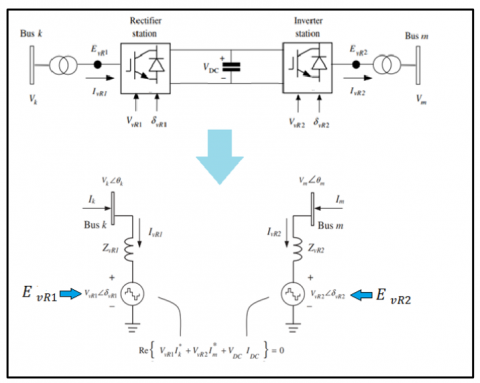
HVDC-VSC consists of two VSC units, one as a rectifier and the other as a converter. The converters are connected either mutually or via a DC cable, depending on the application. It transmits steady DC power to the inverter station from the rectifier. between complex and different frequency networks with high controllability [29]. Figure 2 displays the analogous circuit for HVDC-VSC [24].
One convertor is responsible for controlling the DC voltage, while the other is responsible for transferring the active power across the DC link. The active power flow into the DC system, is equal to the active power entering the AC system at the inverter end minus the losses experienced during the DC cable transfer, as indicated by Eqs. (16) and (17), provided the transformers are loss-free. Both convertors independently manage reactive power during normal operation [30].
Figure 2. VSC-HVDC equivalent circuit [24]
3.2 Power flow analysis for HVDC
In the VSC-HVDC equivalent circuit depicted in Figure 2. The voltage sources which express the two VSC terminals in HVDC according to Eqs. (1) and (2) [31].
So, the power equation for VSC- HVDC without DC line (RDC = 0) is:
$\operatorname{Re}\left\{V_{\mathrm{vR} 1} \mathrm{I}_{\mathrm{vR} 1}^*+\mathrm{V}_{\mathrm{vR} 1} \mathrm{I}_{\mathrm{vR} 2}^*\right\}=0$ (8)
Or the power equation when HVDC-VSC is linked with DC line (RDC > 0) is
$\operatorname{Re}\left\{\mathrm{V}_{\mathrm{vR} 1} \mathrm{I}_{\mathrm{vR} 1}^*+\mathrm{V}_{\mathrm{vR} 1} \mathrm{I}_{\mathrm{vR} 2}^*+\mathrm{P}_{\mathrm{DCloss}}\right\}=0$ (9)
It is assumed the bus k is (rectifier connected terminal) and the bus m is (inverter connected terminal), and that power flows from bus k to bus m.
At the k-bus (at rectifier bus) can express to the active and reactive power equations [24]:
$\begin{aligned} \mathrm{P}_{\mathrm{vR} 1}=V_{k \mathrm{VR} 1}^2 G_{v R 1} & +V_k V_{v R 1}\left[G_{v R 1} \cos \left(\delta_{v R 1}-\theta_k\right)\right. \left.+B_{v R 1} \sin \left(\delta_{v R 1}-\theta_k\right)\right]\end{aligned}$ (10)
$\begin{gathered}\mathrm{Q}_{\mathrm{vR} 1}=-V_{v R 1}^2 B_{v R 1}+V_k V_{v R 1}\left[G_{v R 1} \sin \left(\delta_{v R 1}-\theta_k\right)\right. \left.-B_{v R 1} \cos \left(\delta_{v R 1}-\theta_k\right)\right]\end{gathered}$ (11)
where, the admittance equation $\mathrm{Y}_{\mathrm{vR} 1}=G_{v R 1}+j B_{v R 1}$ where $G_{v R 1}$ and $B_{v R 1}$ represent the conductance and susceptibility of the converter transformer, respectively.
Similarly, for the m-bus (at inverter bus), the power flow is determined by the following equations:
$\begin{aligned} \mathrm{P}_{\mathrm{vR} 2}=V_{k \mathrm{vR}}^2 G_{v R 2} & +V_m V_{v R 2}\left[G_{v R 2} \cos \left(\delta_{v R 2}-\theta_m\right)\right. \\ & \left.+B_{v R 2} \sin \left(\delta_{v R 2}-\theta_{k m}\right)\right]\end{aligned}$ (12)
$\begin{gathered}\mathrm{Q}_{\mathrm{vR} 2}=-V_{v R 2}^2 B_{v R 2}+V_{k m} V_{v R 2}\left[G_{v R 2} \sin \left(\delta_{v R 2}-\theta_m\right)\right. \\ \left.-B_{v R 2} \cos \left(\delta_{v R 2}-\theta_m\right)\right]\end{gathered}$ (13)
3.3 Active and reactive load power calculation in overloaded lines
$\begin{gathered}P G i-P D i-V i \sum V j[G i j \cos (\delta i j)+B i j \sin (\delta i j)]=0 \\ N B j=1 \forall i \in N B\end{gathered}$ (14)
$\begin{gathered}Q G i-Q D i-V i \sum V j[G i j \sin (\delta i j)-B i j \cos (\delta i j)]=0 \\ \forall i \in N B \,\,N B j=1\end{gathered}$ (15)
where, the voltage angle difference between buses $i$ and $j$ is represented by $\delta i j=\delta i-\delta j$, the number of buses is represented by $N B$, and the active and reactive load demands are represented by $P D$ and $Q D$, respectively. The susceptibility between buses $i$ and $j$ is represented by Bij, while the transfer conductance is represented by $G i j$ [32].
3.4 Active and reactive power losses
The total power equation for VSC- HVDC is [33]:
$\mathrm{P}_{\mathrm{vR} 1}+\mathrm{P}_{\mathrm{vR} 2}+\mathrm{P}_{\mathrm{DC}}=0$ (16)
$\Delta P_{H V D C}=\Delta P_{v R 1}-\Delta P_{v R 2}$ (17)
The active power loss for three phase AC system will be:
$\mathrm{P}_{\text {loss}, \mathrm{AC}}=3 * \mathrm{I}^2 * \mathrm{R} *$ distance of route in Km (18)
where, the line current (I) is per phase and the resistance of the conductor is (R), $\Omega / \mathrm{km}$.
The active power loss for two pole DC system will be:
$\mathrm{P}_{\text {loss }, \mathrm{DC}}=3 * \mathrm{I}^2 * \mathrm{R}_{\mathrm{DC}} *$ distance of route in Km (19)
where, the line current (I) is per pole and the resistance of the DC line is RDC, $\Omega / \mathrm{km}$.
3.5 The deployment costs of UPFC and HVDC
UPFC technology is cost-effective in optimizing existing AC grids, reducing congestion, and improving system stability. Therefore, UPFCs can postpone or eliminate the need for costly new transmission projects. Improved system stability also leads to lower operating and maintenance costs [34].
Also can summarize the total cost rate and investment returns.
Where the capital Cost: $20–50 million.
Converter Station Cost: Not required.
Maintenance Cost: Medium (power electronics & cooling) Payback Period (ROI): 5–10 years (depends on power savings & congestion relief) [35].
However, despite its high initial cost, HVDC is a financially feasible option for joining asynchronous grids and transmitting power over vast distances. In hybrid AC/DC systems, power flow can be optimized by combining UPFC and HVDC, offering the best cost-efficiency ratio [36]. In other hand the total cost rate and investment returns can be summaries as [37].
The capital Cost: \$1.0–1.5million/km (overhead),$2.5–5.0 million/km(underground/submarine).
Converter Station Cost: \$100–500 million per terminal Maintenance Cost: Medium to High (valves, converters, insulation systems).
Payback Period (ROI): 10–20 years (depends on project scale).
3.6 The dynamic response of UPFC and HVDC under fault conditions
Power systems, particularly FACTS (Flexible AC Transmission Systems) devices like UPFC and high-voltage transmission systems like HVDC, are greatly impacted by fault conditions like short circuits.
1. UPFC's Response to Fault Situations
Combining a series and a shunt converter, the UPFC offers damping, power flow control, and voltage regulation. Under fault conditions, the shunt inverter provides or absorbs reactive power to maintain voltage stability; the series inverter responds by altering voltage injection to counteract disturbances; and the UPFC improves AC grid stability but requires coordinated control for optimal performance during high-impact short circuits [38].
Therefore, in UPFC-based systems, short-circuit defects result in significant DC-link voltage swings, necessitating quick response control to maintain network stability.
2. Response of HVDC in Fault Situations Because HVDC systems include controlled converters, they are more fault-tolerant than AC transmission. But errors continue to affect the system:
• Because of commutation failure, line commutated converters (LCC-HVDC) have trouble with AC faults [39].
• By utilizing fault ride-through (FRT) and DC choppers, voltage source converters (VSC-HVDC) are better equipped to manage faults.
• DC-side issues necessitate quick-reaction defenses. Fast fault-clearing techniques are necessary because DC-side failures might result in overcurrent surges.
• Although HVDC systems provide more control over power transmission, DC-side faults continue to be a significant problem that necessitates quick fault-clearing techniques.
• UPFC-HVDC techniques for improved fault ride-through performance [40].
To perform as well as possible throughout the study case and during the emergency conditions of the AC network, the selection of the optimal location for the HVDC added to the network has a great impact in terms of improving the voltage, reducing the network losses and the power transmission capacity under overload conditions. Consequently, by identifying the best place to put the UPFC device for HVDC lines, its presence enhances network performance. A genetic algorithm (GA) is used to identify the best site for HVDC transmission and UPFC installation in order to lower overall system power losses and enhance the network's voltage profile (as an objective function) [27]. An objective function f(x) can be defined as a genetic function used to identify problems and develop plans to improve them by starting the natural selection process. Where, $x=x_1, x_2, \ldots x_N$ is a multidimensional vector of optimization data. The better parameters of the genetic algorithm rules are chromosomes and genes. GA encodes the optimization parameters as either a binary string (known as binary encoding) or an array of real values (integers), known as real encoding. A chromosome is a collection of genes that have the following structure:
$\begin{gathered}{ Cromosome }=\left[\begin{array}{c}a_1^1 \\ a_2^1\end{array} \ldots a_{L 1}^1, a_1^2 a_2^2 \ldots a_{L 2}^2, a_1^N a_2^N \ldots a_{L N}^N\right] =\left[x_1, x_2, \ldots . x_N\right]\end{gathered}$
where, $\left[x_1, x_2, \ldots . x_N\right]$ is a multidimensional vector of the optimization coefficient, $a$ is a gene and $L i$ is the length of the code string of the coefficient $i$. The genetic algorithm consists of three basic parts, followed by the crossover rate and mutation operations that are performed until the best population is identified [12, 41].
The optimization control data provided include the population size, crossover and mutation probabilities, iterations, and number of generations. The optimal location for the HVDC and UPFC link is determined by a genetic algorithm that can be introduced into the IEEE-30 & 57 bus system by MATLAB software, and then test system and HVDC and UPFC stations are modelled and simulated based on PSS/E under different load conditions, this can be explain according to following step [12, 42, 43]:
1: Determine the population size in the genetic algorithm and define the network data, UPFC and HVDC.
2: Adopt the energy flow method (Newton Raphson).
3: Find the target values for all individuals.
4: A new population is selected from the old population based on the target values. Based on the calculation function.
5: To create solutions with a new step, the crossover, gene and mutation algorithm operators are applied to the selected population.
6: The goal values for the new chromosomes are determined and applied to the population.
7: If the number of iterations is over, the genetic algorithm program is stopped and the best individual is relied upon, otherwise, move to step 4.
The effectiveness of the suggested genetic algorithm (GA) in determining the best location for the HVDC and UPFC links, respectively, to accomplish all the goals—maximizing balanced power distribution and transmitted power, reducing losses, and improving the voltage profile under various system load conditions—was tested using an IEEE-30 & 57 bus system. The programming language MATLAB R2018a is used to implement GA.
5.1 IEEE-30 bus system
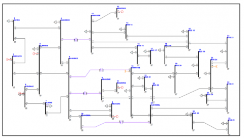
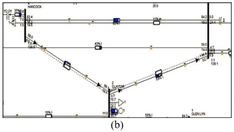
Figure 3 illustrates the standard IEEE 30-bus system, comprising 6 generators, 30 buses, 21 loads, and 41 transmission lines [31], as modeled in the PSS/E software. The UPFC is represented by its two components: one connected to the transmission line to emulate the SSSC functionality and the other connected to the bus to emulate the STATCOM functionality, as shown in Figure 4(b). Similarly, the MT-HVDC system is implemented in the PSS/E software, as depicted in Figure 4.
Figure 3. IEEE 30 bus electrical network configuration
Figure 4. The VSC-HVDC and UPFC in PSS/E applications
In Table 1, it is giving the all-GA parameters values and select the objective function and suitable constrain and applied it in MATLAB (m.file coding) in order to limited the optimal location and size of UPFC and HVDC. For GA to work at its best, population size, crossover rate, and mutation rate must be properly adjusted. For the majority of optimization tasks, sensitivity analysis and comparison experiments recommend balanced population sizes of 100–200, crossover rates of 0.7–0.9, and mutation rates of 0.01–0.05. GA resilience can be further improved by adaptive parameter control techniques (such as self-adaptive mutation) [44, 45].
The PSS/E program is based on the location and appropriate size of UPFC and HVDC to be implemented on the grid and their impact on addressing the problems.
Table 1. Genetic algorithm code parameters
|
Data |
Value |
|
Population size |
80 |
|
Crossover |
0.85 |
|
Fitness limit |
12-14 |
|
Umber of generations |
100 |
The overall active and reactive power requirements of the system in normal case are 283.4 MW and 126.2 Mvar on 100 MVA base and total power active and reactive power generation 301 MW and 134 Mvar. At normal case, the total real and reactive losses are (17.5 MW and 67.6Mvar) and have only one overload transmission line between bus 1 and bus 2 which exceed the normal limit that 100%. While when the loading rate increases by 10%, can find a noticeable increase in the percentage of real and reactive power losses to (22.1 MW and 85.3 Mvar) shown in Table 2.
Table 2. PSS/E result before adding UPFC and MT-HVDC on IEEE-30 bus test system
|
Case |
Loading |
Total Losses |
Over Load Line |
||
|
(MW) |
(Mvar) |
(MW) |
(Mvar) |
||
|
Normal |
283.4 |
126.2 |
17.5 |
67.6 |
1-2 |
|
10% |
312.4 |
139.1 |
22.1 |
85.3 |
1-2 2-6 6-8 |
|
20% |
340.1 |
151.4 |
27.3 |
105.8 |
1-2 2-6 6-8 |
Table 3 shows the overload transmission line and power losses in each line under different load condition before adding UPFC and MT-HVDC on IEEE-30 bus test system.
Table 3. PSS/E result for overload transmission line before adding UPFC and Multi terminal VSC-HVDC on IEEE-30 bus
|
Case |
Overload Line |
Active and Reactive Line Losses |
Overload Line Rating |
|
|
MW |
Mvar |
|||
|
Normal |
(1-2) |
5.18MW |
15.52Mvar |
130% |
|
10% |
1-2 2-6 6-8 |
6.59MW 2.41MW 0.13MW |
19.75Mvar 7.33Mvar 0.47Mvar |
151% 102% 104% |
|
20% |
1-2 2-6 6-8 |
8.20MW 2.97MW 0.16MW |
24.55Mvar 9.01Mvar 0.56Mvar |
168% 112% 111% |
The optimal location of UPFC and Multi terminal VSC-HVDC and the total system losses are given in Tables 4 and 5 respectively. Where the optimal location of UPFC which limited by GA is between bus 3 and 4, and multi terminal VSC – HVDC between bus (6-2) and (4-2) at normal case.
The percentage reduction analysis of active and reactive power losses can be evaluated by:
$(Loss_{{Red.}}=({Loss}_{w o}-{Loss}_w) /{Loss}_{w o} * 100 \%)$
where, the total losses without and with the addition of HVDC (or UPFC) are denoted by the numbers Losswo and Lossw, respectively. It has been shown that the real power losses at normal load condition are decreased by 69.594% after introducing UPFC topology, and after adding multi-terminal HVDC they are decreased by 75%. Also, the reactive power losses are decreased by 74% after adding UPFC and after introducing multi-terminal HVDC topology they are reduced by 78% at the same load.
Table 4. PSS/E result after adding UPFC on IEEE-30 bus test system with GA
|
Case |
Position |
Total Losses |
Over Load Line |
|
|
(MW) |
(Mvar) |
|||
|
Normal |
3-4 |
5.4 |
17.8 |
None |
|
10% |
5-2 |
5.9 |
20.5 |
None |
|
20% |
5-2 10-21 |
7.2 |
23.5 |
None |
Table 5. PSS/E result after adding multi terminal VSC-HVDC on IEEE-30 bus test system with GA
|
Case |
Position |
Total Losses |
Over Load Line |
|
|
(MW) |
(Mvar) |
|||
|
Normal |
6-2 4-2 |
4.3 |
15.2 |
None |
|
10% |
6-2 4-2 |
4.7 |
18.1 |
None |
|
20% |
6-2 4-2 |
5.7 |
23.1 |
None |
In contrast, adding UPFC and Multi terminal VSC-HVDC to the network in the proposed location reduces active and reactive power losses in overloaded transmission lines. This is can show in Tables 6 and 7 were the Overload line rating with UPFC and with VSC-HVDC give best result compare with that in Table 3. For example, at normal case Overload line rating without UPFC and VSC-HVDC is 130%, after adding UPFC between bus (3-4) overload line rating decreases to 40%, while adding the multi terminal VSC-HVDC to network decrease the active power line rating to 39.8%.
Table 6. Overload line, active and reactive line losses with UPFC with GA
|
Case |
Overload Line with UPFC |
Active and Reactive Line Losses with UPFC |
Overload Line Rating with UPFC |
|
|
Normal |
(1-2) |
0.52 MW |
1.56Mvar |
40% |
|
10% |
1-2 2-6 6-8 |
0.92 0.3 0.01 |
2.76 0.91 0.03 |
53% 10% 25% |
|
20% |
1-2 2-6 6-8 |
3.24 1.43 0.03 |
9.7 4.34 0.1 |
95% 75% 48% |
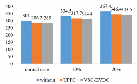
In Figure 5, can show the comparative result for active power generation losses for transmission system under different load conditions, for example at normal operation active power generation 301 MW. After adding UPFC active power generation decreases to 286.2 MW and decrease to 285 Mvar after adding multi terminal VSC- HVDC.
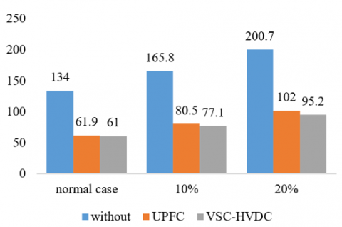
The same effect on reactive power generation will be decreases from 134 Mvar (without any addition) to 61.9 Mvar (with UPFC) to 61 Mvar (with multi terminal VSC- HVDC) this can show in Figure 6.
Table 7. Overload line, active and reactive line losses with MT-HVDC with GA
|
Case |
Overload Line with MT-HVDC |
Active and Reactive Line Losses with MT-HVDC |
Overload Line Rating with VSC-HVDC |
|
|
MW |
Mvar |
|||
|
Normal |
1-2 |
0.450 |
1.50 |
39.8% |
|
10% |
1-2 2-6 6-8 |
0.55 0.23 0.07 |
1.86 0.00 0.26 |
60.3% 10% 25% |
|
20% |
1-2 2-6 6-8 |
0.65 0.23 0.04 |
2.2 0.00 0.16 |
65.8% 13% 20% |
Figure 5. Comparative result for active power generation in transmission system
Figure 6. Comparative result for reactive power generation in transmission system
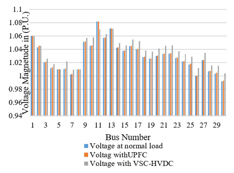
Figure 7. IEEW-30 bus voltage profile under normal loading conditions with and without UPFC and VSC-HVDC
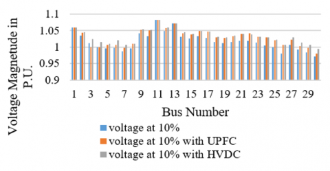
In Figures 7, 8 and 9 at normal load, 10% and 20% increase in the load can show the voltage profile improvement when adding UPFC and VSC-HVDC to the system and not deviations from original values.
Figure 8. IEEE-30 bus voltage profile for a 10% increase in load with and without UPFC and VSC-HVDC
Figure 9. IEEE-30 bus voltage profile for a 20% increase in load with and without UPFC and VSC-HVDC
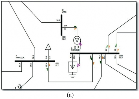
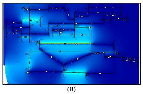
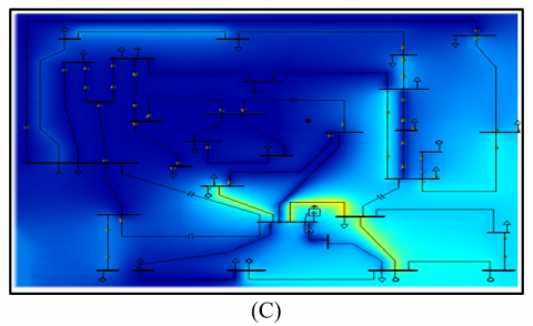
The overload on the transmission line in the IEEE-30 bus system is reduced. the application in PSS/E software using contours and can show the effect of addition UPFC and VSC-HVDC taking at normal operation the overload when the transmission line exceeds more than 100%. can be seen in Figure 10 (a). While Figure 10 (b) and (c) shows the load of the same lines after adding UPFC and VSC-HVDC device.
Figure 10. (A) The loading in IEEE 30 bus transmission line without and addition, (B) With multi terminal VSC-HVDC, (C) With UPFC
5.2 IEEE-57 bus system
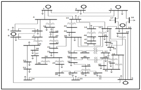
Eighty transmission lines, the generators at buses 1, 2, 3, 6, 8, 9, 12, and fifteen transformers make up the typical IEEE 57-bus system. At buses 18, 25, and 53, the sources of reactive power are taken into account. Figure 11 shows the configuration of the IEEE 57-bus electrical network.
On a 100 MVA basis, the system's overall active and reactive power demands are 1250.8 p.u. and 336.4 p.u. All load bus and generator bus voltages have been limited to between 0.94 and 1.06 p.u.
Figure 11. The configuration IEEE 57 buses electrical network
The overall active and reactive power requirements of the system in normal case are 1250.8 MW and 336.4 Mvar on 100 MVA base and total power active and reactive power generation 1279 MW and 326.3 Mvar. The overall active and reactive losses under typical circumstances are 28.2 MW and 126.2 Mvar, respectively. and have two overload transmission line between bus (1- 2) and bus (8-9) which exceed the normal limit that 100%. While when the loading rate increases by 10%, can find a noticeable increase in the percentage of real and reactive power losses to (41.9 MW and 182.7 Mvar) shown in Table 8.
In Table 9 can show the overload transmission line and power losses in each line under different load condition before adding UPFC and MT-HVDC on IEEE-57 bus test system.
In Tables 10 and 11 can show the optimal location of UPFC and Multi terminal VSC-HVDC and the total system losses. Where the optimal location of UPFC which limited by GA is between bus 8 and 9, and multi terminal VSC – HVDC between bus (8-6) and (8-9) at normal case.
Table 8. PSS/E result before adding UPFC and MT-HVDC on IEEE-57 bus test system
|
Case |
Loading |
Total Losses |
Over Load Line |
||
|
(MW) |
(Mvar) |
(MW) |
(Mvar) |
||
|
Normal |
1250.8 |
336.4 |
28.2 |
126.2 |
1-2 8-9 |
|
10% |
1375.9 |
370 |
41.9 |
182.7 |
1-2 1-15 1-16 8-9 |
|
20% |
1513.5 |
407 |
63.8 |
272.6 |
1-2 2-3 3-4 8-9 1-15 1-16 14-15 |
Table 9. PSS/E result for overload transmission line before adding UPFC and MT-HVDC on IEEE-57 bus
|
Case |
Overload Line |
Active and Reactive Line Losses |
Overload Line Rating |
|
|
MW |
Mvar |
|||
|
Normal |
1-2 8-9 |
1.31 3.19 |
4.41 16.28 |
101% 104% |
|
10% |
1-2 1-15 1-16 8-9 |
1.83 6.67 4.58 3 |
6.19 34.08 20.80 15.29 |
119% 129% 100% 101% |
|
20% |
1-2 2-3 3-4 8-9 1-15 1-16 14-15 |
2.74 8.71 1.41 3 10.91 7.45 2.33 |
9.25 24.84 4.61 15.29 55.77 33.78 7.46 |
145% 116% 128% 101% 166% 128% 116% |
Table 10. PSS/E result after adding UPFC on IEEE-57 bus test system with GA
|
Case |
Position |
Total Losses |
Over Load Line |
|
|
(MW) |
(Mvar) |
|||
|
Normal |
8-9 |
14.5 |
64.4 |
None |
|
10% |
8-9 |
22.9 |
99.0 |
None |
|
20% |
8-9 12-17 |
34.6 |
146.9 |
None |
Table 11. PSS/E result After adding Multi terminal VSC-HVDC on IEEE-57 bus test system with GA
|
Case |
Position |
Loading |
Total Losses |
Over Load Line |
||
|
(MW) |
(Mvar) |
(MW) |
(Mvar) |
|||
|
Normal |
8-6 8-9 |
1250.8 |
336.4 |
12.7 |
56.6 |
None |
|
10% |
8-6 8-9 |
1375.9 |
370 |
18.9 |
83.2 |
None |
|
20% |
8-6 8-9 |
1513.5 |
407 |
29.3 |
124.8 |
None |
Adding UPFC and Multi terminal VSC-HVDC to the network in the proposed location reduces active and reactive power losses in overloaded transmission lines. This is can show in Tables 12 and 13 were the Overload line rating with UPFC and with VSC-HVDC give best result compare with that in Table 9. For example, at normal case Overload line rating without UPFC and VSC-HVDC is 101%, after adding UPFC between bus (8-9) overload line rating decreases to 73%, while adding the multi terminal VSC-HVDC to network decrease the active power line rating to 72%.
Table 12. Overload line, active and reactive line losses with UPFC with GA
|
Case |
Overload Line |
Active and Reactive Line Losses |
Overload Line Rating |
|
|
MW |
Mvar |
|||
|
Normal |
1-2 8-9 |
0.94 0.11 |
3.17 0.47 |
73% 17% |
|
10% |
1-2 1-15 1-16 8-9 |
0.91 2.19 1.69 0.14 |
3.24 11.20 7.65 0.72 |
70% 44% 37% 17% |
|
20% |
1-2 2-3 3-4 8-9 1-15 1-16 14-15 |
1.08 1.65 2.02 0.22 3.96 2.87 1.37 |
3.65 4.70 6.60 1.14 20.24 13.01 4.37 |
88% 29% 59% 17% 89% 50% 58% |
Table 13. Overload line, active and reactive line losses with MT-HVDC with GA
|
Case |
Overload Line |
Active and Reactive Line Losses |
Overload Line Rating |
|
|
MW |
Mvar |
|||
|
Normal |
1-2 8-9 |
0.92 0.03 |
3.09 0.00 |
72% 10% |
|
10% |
1-2 1-15 1-16 8-9 |
0.88 1.83 1.39 0.03 |
2.97 9.37 6.32 0.00 |
65% 39% 32% 10% |
|
20% |
1-2 2-3 3-4 8-9 1-15 1-16 14-15 |
1.01 1.25 1.62 0.03 3.47 2.42 1.30 |
3.40 3.56 5.29 0.00 17.75 10.98 4.17 |
75% 25% 50% 17% 75% 42% 53% |
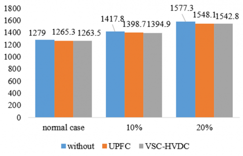
Figure 12 gives the comparative result for active power generation losses for transmission system under different load conditions, for example at normal operation active power generation 1279 MW. After adding UPFC active power generation decreases to 1265.3 MW and decrease to 1263.5 after adding multi terminal VSC- HVDC.
Figure 12. Comparative result for active power generation in transmission system in IEEE-57 bus
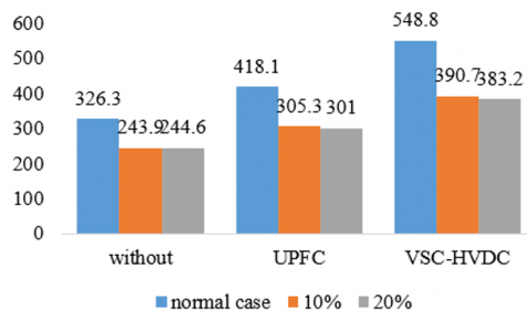
The same effect on reactive power generation will be decreases from 326.3 Mvar (without any addition) to 243.9 Mvar (with UPFC) to Mvar (with multi terminal VSC- HVDC) this can show in Figure 13.
Figure 13. Comparative result for reactive power generation in transmission system in IEEE-57 bus
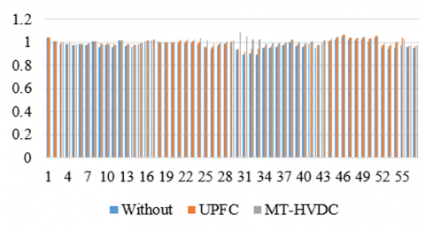
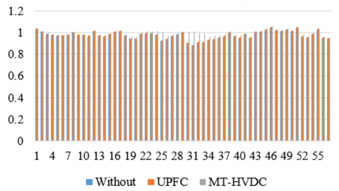
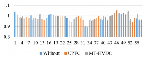
Figure 14. IEEE-57 bus comparison of the voltage profiles under normal loading conditions with and without UPFC and VSC-HVDC
Figure 15. IEEE-57 bus comparison of the voltage profile for a 10% increase in load with and without UPFC and VSC-HVDC
Figure 16. IEEE-57 bus voltage profile comparison with and without UPFC and VSC-HVDC with a 20% increase
In Figures 14, 15 and 16 at normal load, 10% and 20% increase in the load can show the voltage profile improvement when adding UPFC and VSC-HVDC to the system and not deviations from original values.
The results presented in this paper demonstrate that the combined integration of UPFC and Multi-Terminal HVDC significantly enhances the performance of the transmission system. Specifically, these additions reduce total active and reactive power losses, minimize generation losses, maintain system voltage within normal operating limits, and improve transmission line loadability. Both HVDC and UPFC devices are strategically introduced and optimally placed in the system based on the selection criteria provided by a genetic algorithm (GA). A powerful solution for updating electricity networks is the combination of UPFC and HVDC. Effective long-distance transmission is made possible by HVDC, while real-time AC network optimization is offered by UPFC. When combined, they can improve grid dependability, flexibility, and use of renewable energy. Building robust, effective, and sustainable electricity systems will depend heavily on the integration of grid modernization initiatives as they advance.the simulations, conducted in PSS/E, verify a significant decrease in both overall power generation and power losses. Furthermore, under normal load conditions, the VSC-HVDC system outperforms UPFC in terms of voltage profile enhancement and active power loss reduction.
[1] Ackermann, T., Knyazkin, V. (2002). Interaction between distributed generation and the distribution network: operation aspects. In IEEE/PES Transmission and Distribution Conference and Exhibition, Yokohama, Japan, pp. 1357-1362. https://doi.org/10.1109/TDC.2002.1177677
[2] Liang, X., Abbasipour, M. (2022). HVDC transmission and its potential application in remote communities: Current practice and future trend. IEEE Transactions on Industry Applications, 58(2): 1706-1719. https://doi.org/10.1109/TIA.2022.3146117
[3] Radmehr, M., Ghasemi, D., Emami, Y. Power Flow Control in Multi-Terminal VSC-HVDC System. Journal of New Innovations in Electrical Engineering, 2(2):86-94.
[4] Suliman, M.Y., Al-Khayyat, M.T. (2020). Power flow control in parallel transmission lines based on UPFC. Bulletin of Electrical Engineering and Informatics, 9(5): 1755-1765. https://doi.org/10.11591/eei.v9i5.2290
[5] Obabori, S. (2025). High voltage direct current (HVDC) Transmission: Advancing renewable energy integration and long-distance power transfer. Journal of Energy Research and Reviews, 17: 56-68. https://doi.org/10.9734/jenrr/2025/v17i2397
[6] Sivaprasad, G., Reddy, K.R.M. (2012). Optimal power flow using Unified Power Flow Controller (UPFC). International Journal of Electrical and Electronic Engineering & Telecommunications, 1(1): 105-115.
[7] HVDC Links in System Operations. (2019). www.entsoe.eu.
[8] Zaman, I., Basit, A. (2022). High voltage direct current (HVDC) transmission and protection system. International Journal of Engineering Works, 9(5): 124-130. https://doi.org/10.34259/ijew.22.905124130
[9] Oni, O.E., Davidson, I.E., Mbangula, K.N. (2016). A review of LCC-HVDC and VSC-HVDC technologies and applications. In 2016 IEEE 16th International Conference on Environment and Electrical Engineering (EEEIC), Florence, Italy, pp. 1-7. https://doi.org/10.1109/EEEIC.2016.7555677
[10] Roy, A., Dutta, S., Bhattacharya, A., Biswas, S., Chatterjee, R.K., et al. (2024). Frequency constrained optimal power flow incorporating UPFC controller using driving training-based optimization. Research Square. https://doi.org/10.21203/rs.3.rs-4493212/v1
[11] Ogunbowale, P.E., Adejumobi, I.A., Adebisi, O.I., Osinuga, I.A., Fehintola, T.O. (2024). Optimal placement of Unified Power Flow Controller using particle swarm optimization technique. International Journal of Advanced Research, 12(5): 507-520. https://doi.org/10.21474/IJAR01/18742
[12] Hassan, S.K.A., Tuaimah, F.M. (2020). Optimal location of Unified Power Flow Controller genetic algorithm based. International Journal of Power Electronics and Drive Systems, 11(2): 886-894. https://doi.org/10.11591/ijpeds.v11.i2.pp886-894
[13] Kumar, K.A., Reddy, G.S. (2020) Optimal location of HVDC link & UPFC for multi machine power system to improve power system stability. International Journal of Science, Engineering and Technology, 6: 576-581. https://doi.org/10.2348/ijset06150576
[14] Yousuf, S.M., Subramaniyan, M.S. (2013). HVDC and facts in power system. International Journal of Science and Research, 2(12): 133-138.
[15] Gabr, W.I., Dorrah, H.T., El-Gendy, S.A. (2018). Optimal analysis of flexible reconfigurable networks using movable and changeable components. In 2018 Twentieth International Middle East Power Systems Conference (MEPCON), Cairo, Egypt, pp. 69-76. https://doi.org/10.1109/MEPCON.2018.8635104.
[16] Yang, X., Qian, A., Huang, J., An, Y. (2013). Application of multipoint DC voltage control in VSC-MTDC system. Journal of Electrical and Computer Engineering, 2013(1): 257387. https://doi.org/10.1155/2013/257387
[17] Pothisarn, C., Ngaopitakkul, A., Leelajindakrairerk, M., Phannil, N., Bunjongjit, S., Thongsuk, S., Sreewirote, B. (2022). Effects of conditional changes on high-voltage direct current transmission line characteristic. Journal of Electrical and Computer Engineering, 2022(1): 1237997. https://doi.org/10.1155/2022/1237997
[18] Kumar, P., Swarnkar, N.K., Mahela, O.P. (2023). Loss reduction and voltage profile improvement in utility grid using optimal restructuring of transmission network. In 2023 Third International Conference on Advances in Electrical, Computing, Communication and Sustainable Technologies (ICAECT), Bhilai, India, pp. 1-6. https://doi.org/10.1109/ICAECT57570.2023.10118287
[19] Lafta, Y.N., Shalash, N.A., Abd, Y.N., Al-Lami, A.A. (2018). Power flow control of Iraqi international super grid with two terminal HVDC techniques using PSS/E. International Journal of Control and Automation, 11(5): 201-212. https://doi.org/10.14257/ijca.2018.11.5.18
[20] Kanjetawala, S., Kanjetavala, S., Student, P.G. (2013). Unified Power Flow Controller: Modeling, control strategy and control system design. https://www.researchgate.net/publication/318815947
[21] Sadigh, A.K., Hagh, M.T., Sabahi, M. (2010). Unified Power Flow Controller based on two shunt converters and a series capacitor. Electric Power Systems Research, 80(12): 1511-1519. https://doi.org/10.1016/j.epsr.2010.06.015
[22] Li, M., Lin, Z., Wu, W., Lin, Y., Jiang, P., Hu, Z., Du, Y. (2019). Application of UPFC in Fujian 500 kV power grid. The Journal of Engineering, 2019(16): 2510-2513. https://doi.org/10.1049/joe.2018.8576
[23] Revathi, R., Haeden, J.S. (2013). Comparison of GA & PSO in UPFC in A 39 bus network. International Journal of Science and Research, 4(4): 3313-3316.
[24] Vural, A.M., Tümay, M. (2007). Mathematical modeling and analysis of a unified power flow controller: A comparison of two approaches in power flow studies and effects of UPFC location. International Journal of Electrical Power & Energy Systems, 29(8): 617-629. https://doi.org/10.1016/j.ijepes.2006.09.005
[25] Zhang, N., Zhou, Q., Zhao, J. (2021). Optimal location of UPFC based on sensitivity of CDF with power system’s stochasticity. Journal of Engineering Research, 9(2): 149-160. https://doi.org/10.36909/jer.v9i2.8513
[26] Padiyar, K.R. (2007). FACTS controllers in power transmission and distribution. New Age International Publishers.
[27] Acha, E., Fuerte-Esquivel, C.R., Ambriz-Perez, H., Angeles-Camacho, C. (2004). FACTS: Modelling and simulation in power networks. John Wiley & Sons.
[28] Sun, H., Yu, D.C., Luo, C. (2000). A novel method of power flow analysis with Unified Power Flow Controller (UPFC). In 2000 IEEE Power Engineering Society Winter Meeting. Conference Proceedings (Cat. No. 00CH37077), Singapore, pp. 2800-2805. https://doi.org/10.1109/PESW.2000.847327
[29] Rabie, D., Senjyu, T., Alkhalaf, S., Mohamed, Y.S., Shehata, E.G. (2021). Study and analysis of voltage source converter control stability for HVDC system using different control techniques. Ain Shams Engineering Journal, 12(3): 2763-2779. https://doi.org/10.1016/j.asej.2020.12.013
[30] Usman, A.M., Kutay, M., Ercan, T. (2019). MATLAB/SIMULINK model for HVDC fault calculations. In 2019 International Aegean Conference on Electrical Machines and Power Electronics (ACEMP) & 2019 International Conference on Optimization of Electrical and Electronic Equipment (OPTIM), Istanbul, Turkey, pp. 493-499. https://doi.org/10.1109/ACEMP-OPTIM44294.2019.9007154
[31] Zeng, G., Hennig, T., Rohrig, K. (2015). Multi-terminal HVDC modeling in power flow analysis considering converter station topologies and losses. Energy Procedia, 80: 123-130. https://doi.org/10.1016/j.egypro.2015.11.414
[32] Biswas, P.P. (2019). Evolutionary algorithms for solving power system optimization problems. Doctoral dissertation, Nanyang Technological University, Singapore.
[33] Salih, T.K.M., Hussain, Z.S., Ahmed, F.S. (2022). Voltage profile enhancing using HVDC for 132KV power system: Kurdistan case study. Journal of Engineering, 28(1): 52-64. https://doi.org/10.31026/j.eng.2022.01.04
[34] Narain G., Hingorani, Gyugyi, L. (2000). Understanding FACTS: concepts and technology of flexible AC transmission systems. IEEE press.
[35] Marouani, I., Guesmi, T., Hadj Abdallah, H., Ouali, A. (2011). Optimal cost and allocation for UPFC using HRGAPSO to improve power system security and loadability. International Journal of Energy and Environment, 2(5): 813-828.
[36] Liun, E. (2015). Stochastic methodology to estimate costs of HVDC transmission system. Journal of Energy and Power Sources, 2(3): 90-98.
[37] Härtel, P., Vrana, T.K., Hennig, T., von Bonin, M., Wiggelinkhuizen, E.J., Nieuwenhout, F.D. (2017). Review of investment model cost parameters for VSC HVDC transmission infrastructure. Electric Power Systems Research, 151: 419-431. https://doi.org/10.1016/j.epsr.2017.06.008
[38] Kazemi, A., Mahamnia, F. (2008). Improving of transient stability of power systems by supplementary controllers of UPFC using different fault conditions. WSEAS Transactions on Power Systems, 3(7): 547-556.
[39] Cheng, F., Yao, L., Xu, J., Chi, Y., Sun, Y., Wang, Z., Li, Y. (2021). A comprehensive AC fault ride-through strategy for HVDC link with serial-connected LCC-VSC hybrid inverter. CSEE Journal of Power and Energy Systems, 8(1): 175-187. https://doi.org/10.17775/CSEEJPES.2020.03510
[40] Lipu, M.S.H., Karim, T.F. (2013). Effectiveness of FACTS controllers and HVDC transmissions for improving power system stability and increasing power transmission capability. International Journal of Energy and Power Engineering, 2(4): 154-163. https://doi.org/10.11648/j.ijepe.20130204.13
[41] Guvenc, U., Altun, B.E., Duman, S. (2012). Optimal power flow using genetic algorithm based on similarity. Energy Education Science and Technology Part A: Energy Science and Research, 29(1): 1-10.
[42] Merzah, A.N., Abbas, A.H., Tuaimah, F.M. (2024). Enhancing power transmission stability with HVDC systems during load contingencies. Journal Européen des Systèmes Automatisés, 57(1): 177-185. https://doi.org/10.18280/jesa.570118
[43] Shukla, T., Singh, S., Naik, K. (2010). Allocation of optimal distributed generation using GA for minimum system losses in radial distribution networks. International Journal of Engineering, Science and Technology, 2(3): 94-106. https://doi.org/10.4314/ijest.v2i3.59178
[44] Kamil, K., Razali, N.M.M., Teh, Y.Y. (2013). Sensitivity analysis of GA parameters for ECED problem. In 2013 IEEE 7th International Power Engineering and Optimization Conference (PEOCO), Langkawi, Malaysia, pp. 256-260. https://doi.org/10.1109/PEOCO.2013.6564553
[45] Raghavendra, B.V. (2019). Effect of crossover probability on performance of genetic algorithm in scheduling of parallel machines for BI criteria objectives. International Journal of Engineering and Advanced Technology, 9: 2827-2831. https://doi.org/10.35940/ijeat.A9801.109119