Aissa Redhouane Harkat*![]() | Linda Barazane
| Linda Barazane![]() | Abdelkader Larabi
| Abdelkader Larabi![]() | Abdelouadoud Loukriz
| Abdelouadoud Loukriz![]() | Ahmed Bendib
| Ahmed Bendib![]()
© 2025 The authors. This article is published by IIETA and is licensed under the CC BY 4.0 license (http://creativecommons.org/licenses/by/4.0/).
OPEN ACCESS
Optimizing the control of Permanent Magnet Synchronous Motors (PMSMs) is essential for various applications, such as industrial automation, electric vehicles, and renewable energy systems. Conventional control techniques often face difficulties adapting to the nonlinear and dynamic characteristics of PMSMs, resulting in less-than-optimal performance. To overcome these limitations, this study introduces an adaptive nonlinear control (ANLC) approach incorporating a deadbeat observer (DO) to enhance PMSM drive performance. The primary objective is to increase control precision and robustness while accounting for system parameter variations and external disturbances. Comparative simulations between the proposed approach and the conventional ANLC demonstrate its superior capability in handling PMSM operation under fluctuating loads and speed changes. The suggested method reaches a peak relative speed error of approximately 6% at 0.4s when subjected to significantly increasing torque disturbances, outperforming the ANLC, which exhibits an 8% error. Additionally, under significant speed fluctuations at 0.85 s, the proposed control strategy maintains a maximum relative speed error of 0.82%. Furthermore, robustness analysis against variations in system parameters, including stator resistance, inductance, and moment of inertia, confirms the remarkable effectiveness of the developed control method.
deadbeat observer (do), adaptive nonlinear control (anlc), permanent magnet synchronous motor (pmsm), pmsm drive performance enhancement, load torque disturbance
In the dynamic field of modern electrical engineering, it is vital to search for advanced control techniques for electrical machines constantly. Among these machines, the permanent magnet synchronous machine (PMSM) stands out for its high performance, compactness, and exceptional energy efficiency [1]. Its use extends from industrial applications to electric vehicles and renewable energies [2]. Besides, with the development of power electronics and the advance of highly integrated digital control units, several control strategies have been developed [3, 4]. Proportional-integral (PI) loop-based vector control is commonly the industrial standard for PMSM control, owing to its decoupling characteristics and simple structure, which stands out as a powerful and efficient tool that endows the PMSM with dynamic performance as satisfactory as DC machines. However, the PMSM control has a major problem related to the variation of parameters during operation and unknown disturbances, which may threaten the stability of the PMSM drive. Therefore, the control scheme design that can guarantee a safe and stable operation under the mentioned issues is challenging.
Numerous control strategies have been adopted for PMSM control, considering its parameters variation and various disturbances. For instance, an intelligent control strategy employing a recurrent Elman neural network based on the wavelet method (RWENN) is designed for PMSM’s position control, aiming to attain high tracking performance and manage the uncertainties' existence [4]. Indeed, ANNs are a simplified mathematical formulation of biological neurons, but the difficulty of interpreting the behavior of a neural network is a drawback when developing an application. It is also risky to generalize from previous experience and conclude or create rules about how neural networks work and behave. A fuzzy inferior is introduced to adjust the gains of a feed-forward PI controller (Pseudo-derivative feedback with feed-forward gain) [5]. The result of this approach is an appropriate placement of the transfer function closed-loop poles, which improves the ability to reject load torque disturbances. In the 1980s, the first direct torque control (DTC) was introduced [6]. The DTC is a technique applied to PMSMs, capable of providing good electromagnetic torque dynamics. This allows the possibility to achieve these objectives by selecting inverter output vectors from a switching table; stator flux and electromagnetic torque are controlled directly and independently. However, this strategy has significant drawbacks; the switching frequency is not controlled, the presence of large ripples in stator flux and torque, and variations in stator resistance due to temperature change or operation at low rotational speeds may degrade control performance [7]. Therefore, several advanced control techniques have been implemented to enhance the performance of PMSM drive, including the predictive control model (MPC) [8-10], robust control [11-13], sliding mode control (SMC) [14-16], backstepping technique [17-19], adaptive control [20-24], and deep learning algorithms-based control [25-27]. These non-linear control techniques have contributed to improving the PMSM system performance in some ways. On the other hand, recently, observer-based control techniques have gained significant attention for their ability to enhance robustness against load disturbances and parameter uncertainties in PMSMs, emerging as highly popular approaches adopted in the field of AC motor drives [28, 29]. Various observer-based control approaches have been proposed in the literature [30-36]. Although these methods can deliver acceptable performance under perturbation in load torque, the observers’ effectiveness, which depends on precise system models or parameters, tends to diminish when faced with parameter uncertainties.
In the study [30-32, 37], model-based reduced-order nonlinear observers-based controllers, including linear extended observer, extended-order nonlinear observer (ENO), and state-observer, have been developed to enhance robustness versus load torque perturbation with slow variation. Nevertheless, these observers-based control techniques exhibit sensitivity to parameter changes. In [33-35], reduced-order, linear extended state, and linear extended high-gain observers have been employed to accomplish satisfactory performance under load torque disturbances and provide strong robustness versus several parameter uncertainties. Nevertheless, some parameters still need to be precisely known.
To enhance the performance of controllers based on observer that relies on accurately known parameters, techniques insensitive to system parameters have been adopted [38-49]. Such methods not only offer strong robustness under load torque disturbance but also enhance performance with system parameter uncertainties. In [38, 39], extended sliding-mode and terminal sliding-mode observers have been introduced to estimate load torque and mechanical PMSM parameters. As electrical parameters can be measured more easily by employing sensors or instruments compared to mechanical parameters, the focus is primarily on estimating the mechanical parameters. However, electrical parameters often change with time due to factors such as temperature fluctuations, cross-saturation effects, and magnetic saturation, making them difficult to accurately determine during operation [40-42]. A combination of SMC and a disturbance observer has been adopted to tackle time-varying disturbances and parameters [43]. However, the controllers’ and observers’ parameters tuning is complicated and time-demanding, and it also lacks validation under parameter uncertainties. In [44, 45], disturbance observer-based techniques have been designed to improve the PMSM control performance under disturbances and uncertainties, but test results for parameter uncertainties have not been provided. In [46, 47], nonlinear disturbance and extended nonlinear observers have been introduced for estimating specific parameters and load torque, but practical results were missing. A design of an automatic disturbances’ rejection controller based on an extended state observer has been explored for high-performance PMSM robust motion control, focusing on the control of position [48]. An innovative control structure utilizing dual proportional-integral (PI) observers has been developed to maintain operation with high performance in the presence of parameter uncertainties and slowly varying disturbances [49]. In [34, 50, 51], a high-order sliding mode observer, a comprehensive disturbance observer, and an adaptive observer of stator current and disturbance have been proposed to improve the PMSM control performance, ensuring high robustness under disturbances and parameter uncertainties. Beyond the aforementioned techniques, a nonlinear adaptive control approach incorporating high-gain states and an observer of perturbation has been successfully implemented in various applications [52, 53]. This method ensures acceptable performance even versus model or parameter uncertainties, as well as load disturbances.
Furthermore, to improve the robustness of the SMC, a design of a sliding mode speed controller considering a novel variable rate exponential reaching law is suggested [54]. Subsequently, an extended state observer is employed to extract and compensate for parameter mismatches and external disturbances. This approach results in a novel sliding mode predictive current control strategy, which not only maintains the fast dynamic response of the current control but also significantly improves the system's robustness.
Considering this literature review, the primary objective of our research is to develop a control law for the PMSM that enhances performance in trajectory tracking, disturbance rejection, stability, robustness against parameter uncertainties, adherence to physical, and computational efficiency while preserving the inherent non-linear characteristics of the system. In addition, it is known that the control by linearization between outputs strategy suffers from a lack of robustness to external disturbances and model imperfections. Therefore, a novel hybrid adaptive nonlinear control with a specifically tailored DO technique is proposed in this paper, aiming to enhance the control performance of PMSMs. The key innovation lies in the integration of linear and nonlinear control methodologies, facilitated by the utilization of a DO for real-time state estimation. Unlike traditional control approaches, which often struggle to adapt to the dynamic and nonlinear characteristics of PMSMs, the proposed method aims to provide a more effective and robust solution. The novelty of our approach is represented by its ability to dynamically adapt to system variations and disturbances while maintaining precise control over PMSM. By leveraging the real-time state estimation capabilities of the DO, the proposed strategy can generate control signals that accurately track desired references, even in the presence of changing load conditions and speed fluctuations. This adaptive nature of the proposed strategy makes it particularly well-suited for applications where precise control of PMSMs is essential, such as electric vehicles, industrial automation, and RESs.
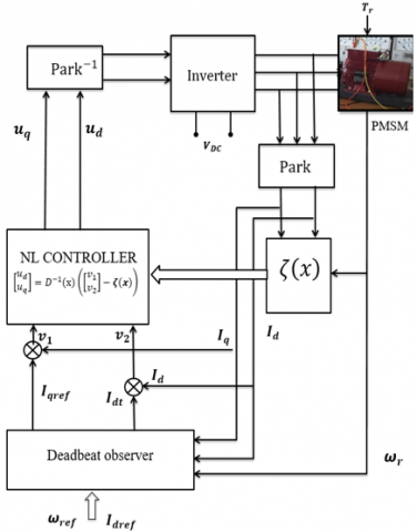
Figure 1 depicts the structure of the PMSM with the proposed control scheme. The PMSM is fed by a DC source via an inverter. A PWM block that handles the voltage references in the abc frame provides the switches' commands of the inverter. The abc voltage references are obtained by transferring the dq voltage references generated by the proposed ANLC scheme. The proposed ANLC scheme is composed of (i) two PI regulators intended for controlling the current direct component, id, and the rotor motor speed, ωr, to their references, and (ii) an incertitude calculation block in charge of determining the incertitude of the speed and current. Note that the ANLC voltage references in the dq frame result from adding the output voltage of the two regulators to the voltages generated by the uncertainty block. The proposed DO in this scheme is responsible for estimating the motor speed and the current in the dq frame from the measured currents.
The PMSM’s modeling is provided in the following subsection, while the detailed analysis of the blocks within the developed control scheme will be presented in the next section.
2.1 PMSM model
Given the simplifying PMSM assumptions, the PMSM model in the dq frame is given by:
$\left\{\begin{array}{c}\frac{d}{d t} I_d=-\frac{R_s}{L_d} I_d+\boldsymbol{p} \omega_r \frac{L_q}{L_d} I_q+\frac{u_d}{L_d} \\ \frac{d}{d t} I_q=-\frac{R_s}{L_q} I_q-\boldsymbol{p} \omega_r \frac{L_d}{L_q} I_d-\frac{1}{L_q} \varphi_f \omega_r+\frac{u_q}{L_q} \\ \frac{d}{d t} \omega_r=\frac{K_T}{J} I_q+\frac{K_T\left(L_d-L_q\right)}{J \varphi_f} I_d I_q-\frac{f}{J} \omega_r+\frac{T_r}{J}\end{array}\right.$ (1)
where, $I_{d q}$ and $u_{d q}$ are the inverter output current and voltage in the $d q$ frame, $L_{d q}$ is the stator inductance, $R_s$ is stator resistance, $T_r$ is the resistive torque, $\omega_r$ is the rotor speed, $f$ is the viscous friction coefficient, $J$ is the machine's total moment of inertia, $p$ denotes the number of pole pairs, $K_T$ is a constant which equals $\frac{3}{2} \boldsymbol{p} \varphi_f$, and $\varphi_f$ is magnetic flux.
Figure 1. Structure of the studied PMSM system with the proposed adaptive nonlinear control with a deadbeat observer [39]
In the context of the control of complex dynamic systems, such as the system of a PMSM, the application of the proposed non-linear adaptive control with a DO offers a robust and efficient solution. This approach, specifically adapted to the PMSM, enables the control parameters to be dynamically adjusted to suit variations in the system while guaranteeing fast and accurate estimation of the internal states, thanks to the DO. By combining these advanced techniques, it is possible to achieve optimum performance even in dynamic and non-linear environments in automotive electric propulsion. In the proposed scheme, the adaptive nonlinear controller combines the nonlinear technique of input-output looping linearization and the adaptive linear control method to ensure the tracking of system reference trajectories with parametric uncertainties.
Meanwhile, the DO is introduced to ensure an accurate estimation of the current dq components and the PMSM speed using the actual measured currents.
In the following subsections, the design of the nonlinear controller is described in detail, considering variations of the system's parameters and load disturbances for non-adaptive and adaptive controller cases. In addition, the operation principle of the adopted DO is discussed.
3.1 Design of the adaptive nonlinear controller
The design of the nonlinear controller is established by considering the uncertainty of the different parameters. The first case considers a linear uncertainty of stator resistance and load torque. The second one inspects the inductances and moment of inertia uncertainty, which are non-linear, as they are difficult to measure exactly. In these studied cases, both non-adaptive and adaptive controllers are investigated.
3.1.1 Case of variations on R and Tr
Here, the aim is to design an adaptive non-linear controller that guarantees speed regulation of the PMSM with constant but unknown stator resistance Rs and resistive torque Tr. To achieve this, we start by designing a controller using the linearization method applied to the input-output dynamics of the nominal PMSM model. Then, we derive the adaptation law to extract the vector of uncertain parameters. The vector of uncertain parameters, λ, is considered as follows:
Then, the system of (1) can be rewritten in the expression given in (3), which proposes an adaptive scheme for estimating Rs and Tr. By replacing (2) in (1), we get:
$[\lambda]=\left[\begin{array}{l}\lambda_1 \\ \lambda_2\end{array}\right]=\left[\begin{array}{l}R-R_n \\ T_r-T_{r n}\end{array}\right]$ (2)
$\left\{\begin{array}{c}\frac{d}{d t} I_d=-\frac{R_n}{L_d} I_d+\lambda_1 \frac{I_d}{L_d}+p \omega_r \frac{L_q}{L_d} I_q+\frac{u_d}{L_d} \\ \frac{d}{d t} I_q=-\frac{R_s}{L_q} I_q-\lambda_1 \frac{I_d}{L_d}-\boldsymbol{p} \omega_r \frac{L_d}{L_q} I_d-\frac{p \omega_r}{L_q} \varphi_f+\frac{u_q}{L_q} \\ \frac{d}{d t} \omega_r=\frac{K_T}{J} I_q+\frac{K_T\left(L_d-L_q\right)}{J \varphi_f} I_d I_q-\frac{f}{J} \omega_r-\frac{T_{r n}}{J}-\frac{\lambda_2}{J}\end{array}\right.$ (3)
where, the subscript n denotes nominal values.
In a compact form:
$\dot{X}=f(X, \lambda)+\sum_{i=1}^2 g_i(X, \lambda) u_i$ (4)
$\dot{X}=f_0(X)+\sum_{i=1}^2 g_i(X, \lambda) u_i+\sum_{i=1}^2 \lambda_j f_{\lambda_j}(x)$ (5)
Non-adaptive controller case
This subsection provides the design of the controller’s non-adaptive version, where the vector of uncertain parameters is known. The objective is to ensure PMSM speed control while maintaining operation at maximum torque (Id= 0). To this end, a linearization law in the input-output directions is applied to its model, which guarantees total decoupling between inputs and outputs. The system outputs are the mechanical speed ωr and the current Id, which are defined as follows:
$\left\{\begin{array}{l}y_1=h_1=I_d \\ y_2=h_2=\omega_r\end{array}\right.$ (6)
These two outputs should follow the reference trajectories. For the current (Id), it is zero (Id = 0), while the speed reference may be a step or any trajectory.
To establish the decoupling matrix D(x), we start by determining the relative degree of each output to be controlled.
Relative degree: For current $I_d$ with $y_1=h_1=I_d$, $\nabla h_1=\left[\begin{array}{lll}1 & 0 & 0\end{array}\right]$, using (4), we get:
$\dot{y}_1=L_f h_1(x)+\sum_{i=1}^2 L_{g_i} h_1(x) u_i$ (7)
Note that the $u_d$ input appears in (7); stop here and take the relative degrees of this output $r_1=1$.
For speed $\omega_r$ with $y_2=h_2=\omega_r$ and $\nabla h_2=\left[\begin{array}{lll}\mathbf{0} & \mathbf{0} & 1\end{array}\right] ;$
Note that if the problem involves finding a linear relationship between input and output, derive the output until at least one input appears by using the following expression:
$\begin{gathered}y_j^{\left(r_j\right)}=L_j^{\left(r_j\right)} h_j(x)+\sum_{i=1}^p L_{g_i}\left(L_j^{\left(r_j-1\right)} h_j(x)\right) u_i ; i=1,2, \ldots \ldots p\end{gathered}$ (8)
If $L_j^{\left(r_j-1\right)} h_j(x) \neq 0$, so $u_i$ does not appear in the $y_j, \dot{y}_j, \ldots . y_j^{\left(r_j-1\right)}$ and appears in the equation of $y_j^{\left(r_j\right)}$.
In this case, $\left(r_j\right)$ is called the system relative degree. According to the following definition, using (9), we get:
$\dot{y}_2=L_f h_2(x)+\sum_{i=1}^2 L_{g_i} h_2(x) u_i$ (9)
Note that no input appears in (10), so we are forced to derive another time:
From (10), $r_2=2$ for this output.
The total relative degree (global or vector) $r_1+r_2=r=3$, so the system is exactly linearizable for non-linear state feedback. There are no internal or unobservable zero dynamics to consider. By putting together (7) and (10), we obtain the following form
$\ddot{y}_2=L^2{ }_f h_2(x)+\sum_{i=1}^2 L_{g_i} h_2(x) u_i$ (10)
$\left[\begin{array}{ll}\dot{y}_1 & \ddot{y}_2\end{array}\right]^T=\zeta(x)+D(x) u$ (11)
where, the decoupling matrix is invertible if the determinant det (D(x) ≠ 0), which equals:
$|D(x)|=\frac{3 p}{2 J L_q L_d}\left(\varphi_f+I_d\left(L_d-L_q\right) \neq 0\right.$ (12)
The linearizing control law that guarantees decoupling between inputs and outputs (i.e., a linear relationship) is:
$\left[\begin{array}{l}u_d \\ u_q\end{array}\right]=D^{-1}(\mathrm{x})\left(\left[\begin{array}{l}v_1 \\ v_2\end{array}\right]-\boldsymbol{\zeta}(\boldsymbol{x})\right)$ (13)
Replacing the linearizing control law (13) in (10) gives:
$\left[\begin{array}{l}\dot{y}_1 \\ \ddot{y}_2\end{array}\right]=\left[\begin{array}{c}\dot{I}_d \\ \ddot{\omega}_{r_2}\end{array}\right]=\left[\begin{array}{l}v_1 \\ v_2\end{array}\right]$ (14)
So, in the case of a trajectory tracking problem, the new control vector is designed.
Conception of the new control vector: For the reference trajectory tracking problem, the vector v must satisfy:
$\begin{aligned} v_j=y_{d j}^{\left(r_j\right)}+ & K_{r j}\left(y_{d j}^{\left(r_j-1\right)}-y_j^{\left(r_j-1\right)}\right)+\cdots +K_1\left(y_{d_j}-y_j\right) 1 \leq j \leq p\end{aligned}$ (15)
where, the vectors $\left(y_{d_j}, y_{d_j}^{\cdot}, \ldots, y_{d j}^{\left(r_j-1\right)}, y_{d j}^{\left(r_j\right)}\right)$ are the reference trajectories imposed for each output.
So, according to (15), we have:
The Laplace transformation of (16) leads to:
$v_1=I_d^*+K_d\left(I_d^*-I_d\right)$ (16)
$v_2=\ddot{\omega}_r^*+K_2\left(\dot{\omega}_r^*-\dot{\omega}_r\right)+K_1\left(\omega_r^*-\omega_r\right)$ (17)
$s+K_d=0$ (18)
Also, applying the Laplace transformation to (17) gives:
$s^2+K_{2 s}+K_1=0$ (19)
To determine the coefficients $K_d, K_1$, and $K_{2 S}$ we use the pole placement method so that the system is stable and its output responds without any overshoot. If the reference trajectory (the imposed trajectory) is a step, we have $I_d^*=$ $\ddot{\omega}_r^*=\dot{\omega}_r^*=0$, and the control vector becomes:
$\begin{gathered}v_1=K_d\left(I_d^*-I_d\right) \\ v_2=-K_2 \dot{\omega}_r+K_1\left(\omega_r^*-\omega_r\right)\end{gathered}$ (20)
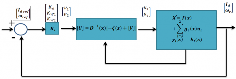
Accordingly, the block diagram of the linearized closed-loop model can be derived, as shown in Figure 2.
Figure 2. Block diagram of the linearized closed-loop model
Adaptive controller case
Since $\lambda$ is unknown, it is replaced by its estimate $\hat{\lambda}$, which is proposed for the design. Accordingly, the output vectors are:
$\left[\begin{array}{ll}y_1 & y_2\end{array}\right]^T=\left[\begin{array}{ll}I_d & \omega_r\end{array}\right]^T=\left[\begin{array}{ll}\varphi_1 & \varphi_2\end{array}\right]^T=\left[\begin{array}{ll}h_1 & h_2\end{array}\right]^T$ (21)
The change of coordinates according to $\hat{\lambda}$ is defined as follows:
$[\hat{z}]=\left[\begin{array}{c}L_{f_0} \varphi_1 \\ L_{f_0} \varphi_2 \\ L_{f_0}^2 \varphi_3\end{array}\right]+\left[\begin{array}{cc}L_{g_1} \varphi_1 & 0 \\ 0 & 0 \\ L_{g_1} L_{f_0} \varphi_2 & L_{g_2} L_{f_0} \varphi_2\end{array}\right]\left[\begin{array}{l}u_d \\ u_q\end{array}\right]$ (22)
According to expression (22), we have:
$\left\{\begin{array}{l}R=\lambda_1+R_n \\ T_r=\lambda_2+T_{r n}\end{array}\right.$ (23)
By replacing Eq. (22) in (23), we obtain the dynamics of Z as follows:
$\left[\begin{array}{c}\hat{\dot{Z}}_1 \\ \hat{\dot{Z}}_2 \\ \hat{\dot{Z}}_3\end{array}\right]=\left[\begin{array}{c}L_{f_0} \varphi_1+\lambda_1 L_{f_{\delta_1}} \varphi_1 \\ L_{f_0} \varphi_2+\lambda_2 L_{f_{\delta_2}} \varphi_2 \\ L_{f_0}^2 \varphi_3+\lambda_1 L_{f_{\lambda_1}} L_{f_0} \varphi_2+\lambda_2 L_{f_{\lambda_2}} L_{f_0} \varphi_2+\hat{\lambda}_2 L_{f_{\delta_2}} \varphi_2\end{array}\right]+\left[\begin{array}{cc}L_{g_1} \varphi_1 & 0 \\ 0 & 0 \\ L_{g_1} L_{f_0} \varphi_2 & L_{g_2} L_{f_0} \varphi_2\end{array}\right]\left[\begin{array}{l}u_d \\ u_q\end{array}\right]$ (24)
where, the decoupling matrix is given by:
$L_{f_{\lambda_1}} \varphi_1=-\frac{1}{L_d} I_d$ (25)
Our controller depends on $\lambda$, which is not yet determined, so the linearizing law becomes, in this case:
$\left[\begin{array}{l}\hat{u}_d \\ \hat{u}_q\end{array}\right]=D^{-1}(x)\left(-\zeta_0(x)-\zeta_\delta(x, \hat{\lambda}, \hat{\lambda})+\hat{v}\right)$ (26)
To adjust our adaptive controller using the Lyapunov-based adjustment mechanism, we need to define the state error vector, which is given by:
That should satisfy the following condition:
$e=\left|\begin{array}{c}I_d-I_d^* \\ \omega_r-\omega_r^* \\ \omega_r-\dot{\omega}_r^*\end{array}\right|=\left[\begin{array}{l}e_1 \\ e_2 \\ e_3\end{array}\right]$ (27)
$e=K \dot{e}+W_1 \Delta \lambda$ (28)
where, K is a matrix that depends on the desired poles, and from (24), we define $W_1$ as follows:
$W_1=\left[\begin{array}{cc}-\frac{1}{L_d} I_d & 0 \\ 0 & -\frac{1}{\mathrm{~J}} \\ -\left(\frac{K_T}{J L_q} I_q+\frac{K_T\left(L_d-L_q\right)}{J \varphi_f L_q} I_q I_d\right)-\left(\frac{K_T\left(L_d-L_q\right)}{J \varphi_f L_d} I_q I_d\right) & \frac{f}{J^2}\end{array}\right]$ (29)
Thus, the adaptation law can be determined using the following Lyapunov function:
$V=e^T P e+\Delta \lambda^T \Gamma \Delta \lambda$ (30)
where, its derivative is given by:
$\frac{d V}{d t}=-e^T Q_e+2 \Delta \lambda^T\left(W_1^T P e+\Gamma \Delta \dot{\lambda}\right)$ (31)
and Γ and P are positive-definite matrices defining the adaptation gain and the solution to the Lyapunov equation, respectively.
So that $\frac{d V}{d t} \leq 0$ it is necessary:
$W_1 P e+\Gamma \Delta \dot{\lambda}=0 \rightarrow \Delta \dot{\lambda}=-\Gamma^{-1} W_1^T P e$ (32)
where, $\Delta \dot{\lambda}$ represents the adaptation act, which ensures:
$\frac{d V}{d t}=-e^T Q_e \leq 0$ (33)
In this case, according to the Barbalat lemma, we have:
$\lim _{t \rightarrow \infty}\|e(t)\|=0$ (34)
So, now it remains to determine the matrix P, which verifies the following equation:
$K^T P+P K=-Q$ (35)
where, Q is a positive-definite symmetric matrix that is generally an identity matrix.
3.1.2 Case of variations on (Ld = Lq) and J
In this case, the steps to design the controller are similar to those in the previous section, considering L and J variations, which are involved within the PMSM model in a non-linear way. Thus, the vector of uncertain parameters is considered as follows:
$\lambda=\left[\begin{array}{l}\lambda_1 \\ \lambda_2\end{array}\right]=\left[\begin{array}{l}\frac{1}{L}-\frac{1}{L_n} \\ \frac{1}{J}-\frac{1}{J_n}\end{array}\right]$ (36)
$\left\{\begin{array}{l}L=\frac{L_n}{L_n \lambda_1+1} \\ J=\frac{J_n}{J_n \lambda_2+1}\end{array}\right.$ (37)
Note that from (36), the vector $\lambda$ denotes the difference between the uncertain parameters and their nominal values, so to obtain the values of $L$ and $J$ from $\lambda_1$ and $\lambda_2$, the following expressions can be used:
3.2 Deadbeat state observer
The DO is designed to estimate the unmeasured states of the system at each instant. In the case of the PMSM, the states typically estimated are the stator currents, $\hat{I}_d$ and $\hat{I}_q$, and the rotational speed $\widehat{\omega}_r$. The state estimates equations of the DO can be formulated as follows:
$\left\{\begin{array}{c}\hat{x}(k+1)=A \hat{x}(k)+B u(k)+L(y(k)-C \hat{x}(k)) \\ \hat{x}(0)=x_0\end{array}\right.$ (38)
with: $\hat{x}(k)$: the vector of the estimated states at time $k ; A$: the system state matrix; $B$: the control matrix; $u(k)$: the control vector at time $k ; L$: the DO gain matrix; $y(k)$: the output vector measures at time $k$; and $C$: The output matrix.
3.2.1 Design of the control parameters for the DO
The system state matrix can be derived from its dynamic model in the dq frame, which is defined as follows:
$\begin{aligned} \frac{d}{d t}\left[\begin{array}{c}I_d \\ I_q \\ \omega_r\end{array}\right]= & {\left[\begin{array}{ccc}-\frac{R}{L_d} & \omega_r & 0 \\ -\omega_r & -\frac{R}{L_q} & \frac{1}{L_q} \varphi_f \\ 0 & -\frac{1}{J} \frac{d L}{d \omega_r} & \frac{-f}{J}\end{array}\right]\left[\begin{array}{c}I_d \\ I_q \\ \omega_r\end{array}\right] } +\left[\begin{array}{cc}\frac{1}{L_d} & 0 \\ 0 & \frac{1}{L_q} \\ 0 & 0\end{array}\right]\left[\begin{array}{l}u_d \\ u_q\end{array}\right]\end{aligned}$ (39)
The state matrix A is, therefore, the part of the dynamic model that determines the evolution of system states over time. Using the equations above, we can extract the elements of the A matrix:
$A=\left[\begin{array}{ccc}-\frac{R}{L_d} & \omega_r & 0 \\ -\omega_r & -\frac{R}{L_q} & \frac{1}{L_q} \varphi_f \\ 0 & -\frac{1}{J} \frac{d L}{d \omega_r} & \frac{-f}{J}\end{array}\right]$ (40)
For a PMSM, the state vector estimates $\hat{x}$ and the matrix B can be obtained as:
$\hat{x}=\left[\begin{array}{l}\hat{I}_d \\ \hat{I}_q \\ \widehat{\omega}_r\end{array}\right], B=\left[\begin{array}{cc}\frac{1}{L_d} & 0 \\ 0 & \frac{1}{L_q} \\ 0 & 0\end{array}\right]$ (41)
In the matrix B, each column represents the effect of the input voltage on the corresponding states of the system. Rows 1 and 2 correspond to the currents $L_d$ and $L_q$, respectively, while row 3 corresponds to the rotational speed $\omega_r$. The non-zero elements of this matrix B indicate how the input voltage components influence the different state variables of the system. For example, the input voltage $u_d$ affects only the current $(I)$, so only the first column of matrix $B$ has non-zero elements corresponding to $L_d$. Similarly, the input voltage $u_q$ affects only the current, so only the second column of matrix $B$ has non-zero elements corresponding to $L_q$. The rotational speed $\omega_r$ is not directly affected by the input voltage, so the third column of matrix $B$ is zero. The matrix $B$ is important in designing control laws for PMSMs because it indicates how the system inputs (the voltages $u_d$ and $q$ in this case) influence the system states, which is essential for designing an effective controller.
Observation matrix C
The matrix C is used to select the states that can be measured. In the case of the PMSM, let's assume we can directly measure the currents as well as the mechanical rotational speed $\omega_r$. Then, the matrix C would be:
$C=\left[\begin{array}{lll}1 & 0 & 0 \\ 0 & 1 & 0 \\ 0 & 0 & 1\end{array}\right]$ (42)
Design of the gain matrix L of the DO
To design the gain matrix L of the DO for a PMSM, we can use the classical state observer design method, such as the pole placement method. This method consists of placing the poles of the estimation error dynamics where we want them to obtain a fast and stable observer’s convergence. The estimation error dynamics is given by the equation:
$\tilde{\dot{x}}=(A-L C) \tilde{x}$ (43)
In which $\tilde{x}$ defines the estimation error vector:
$\tilde{x}=x-\hat{x}$ (44)
where, $\boldsymbol{x}$ and $\hat{x}$ are the actual state vector and the state estimate vector.
The matrix L can be calculated for an n-dimensional system using:
$L=(A-L C)^{-1} B$ (45)
Thus, to calculate the matrix L, we need to follow the following steps:
Choose the desired eigenvalues $\lambda_1, \lambda_2 \ldots \lambda_{\mathrm{n}}$:
More precisely, for a nonlinear dynamic system such as that of a PMSM, the eigenvalues λ of the matrix A-LC determine the dynamics of the state observer's estimation errors:
$\operatorname{det}(z I-(A-L C))=0$ (46)
$\tilde{\dot{x}}=(A-L C) \tilde{x}$ (47)
If the eigenvalues λ have a negative real part, this means that the estimation errors will decrease over time, indicating stable convergence of the estimation to the real values of the system states. In other words, the PMSM will tend to track the real values of its states quickly and accurately with a well-designed observer.
By judiciously choosing the eigenvalues λ, we can control the observer's performance, such as speed of convergence and robustness to disturbances. For example, if faster response times are required, we can choose eigenvalues with a more negative real part, which will speed up the observer's convergence. The approach proposed in this article enables the matrix L to be calculated as a function of the specific PMSM’s parameters and the observer’s specifications, providing an accurate estimate of the internal states of the PMSM for fast, stable convergence of the observer.
3.2.2 Application of the nonlinear adaptive deadbeat control
Before delving into the integration process, it's crucial to understand the context of designing and applying nonlinear adaptive input-output feedback control with DO for PMSMs. This control approach aims to regulate PMSM performance effectively using advanced control and state estimation methods. The system relies on a DO to estimate unmeasured states, enabling precise and rapid feedback. The integration of this control occurs in four distinct steps, each playing a crucial role in the overall dynamics of the system. The main steps of the DO are given as follows.
$\widehat{\boldsymbol{x}}(k+1)=A \widehat{\boldsymbol{x}}(k)+B u(k)+L(y(k)-C)$ (48)
$v(k)=-\Gamma \hat{\boldsymbol{x}}(k)$ (49)
where, Γ is the adaptive gain matrix cited in the above part.
$\begin{aligned} u(k)= & -K_p\left(y(k)-y_{r e f}(k)\right) -K_i \int\left(y(k)-y_{r e f}(k)\right) d t +v(k)\end{aligned}$ (50)
$\left\{\begin{aligned} \Gamma(k+1)= & \Gamma(k)+\mu\left(y(k)-y_{r e f}(k) \widehat{x}(k)^T\right. \\ & \varepsilon=y(k)-y_{\text {ref }}(k)\end{aligned}\right.$ (51)
where, $\mu$ is the learning factor.
The equation for the learning factor (μ) in the LMS with the stochastic gradient descent (SGD) algorithm for updating the adaptive parameters of the Γ(x) matrix is as follows:
$\mu=\delta /\|\hat{x}(k)\|^2$ (52)
with δ is a positive parameter that controls the learning speed and $\|\hat{x}(k)\|^2$ is the Euclidean norm of the state estimation vector $\hat{x}(k)$.
Note that δ controls the learning speed. A larger δ means a faster update of the adaptive parameters, while a smaller δ means a slower update. While $\|\hat{x}(k)\|^2$ is used to normalize the updating of adaptive parameters. This prevents the adaptive parameters from becoming too large or too small.
To validate the performance of the developed control strategy, simulation tests are established in MATLAB software. In the first test, a comparative study with an ANLC technique is conducted to check the effectiveness of the proposed controller under mechanical rotation speed variation and load torque disturbance. The second test verifies the robustness of the control proposal considering the system parameters variation. Note that our study focuses on non-salient PMSM and the corresponding parameters are provided in Table 1.
4.1 Control performance assessment under speed variation and load torque disturbance
In this simulation test, a comparative study between the proposed control and a simple ANLC technique for three different scenarios is performed. These scenarios are presented hereafter, which consider constant values and variations of the mechanical rotation speed and load torque disturbance as well.
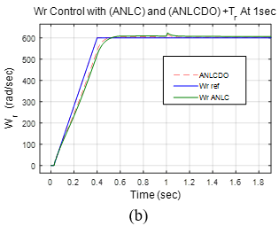
4.1.1 Scenario 1: Fixed mechanical rotational speed with unknown load torque perturbation:
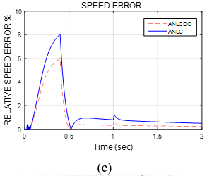
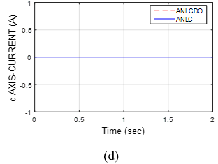
Here, we subject the system to a gradually varying unknown load torque perturbation with an unchanged mechanical rotational speed to evaluate the system control robustness versus these disturbances. The load torque, Tr, the mechanical speed, ωr, and its reference are portrayed in Figures 3(a) and (b). Figures 3(b) and (c) reveal the superior performance of the developed control approach in tracking the mechanical speed, even under a significant perturbation in load torque. Moreover, both methods keep the current at zero.
The maximum relative error, expressed as $\left|\frac{\omega_r-\omega_{r e f}}{\omega_{r e f}}\right| \times 100 \%$, is approximately 8% and 6% for the ANLC and the proposed method, respectively, at time 0.4 s. In addition, at time 1 s, the error decreases to 1.2% and 0.7% for the ANLC and the proposed control scheme, respectively.
Table 1. PMSM parameters
|
Parameter |
Value |
|
Nominal power (Pn) |
1,1 kW |
|
Number of pole pairs (p) |
4 |
|
Stator resistance (Rs) |
1.8 Ω |
|
Direct inductance component (Ld) |
2.89 mH |
|
Quadrature inductance component (Lq) |
2.89 mH |
|
Magnet flux |
0.416 Wb |
|
Friction coefficient (fr) |
0.000125 Nms/rad |
|
Moment of inertia (J) |
0.011 kgm2 |
|
Nominal speed (Nn) |
1500 tr/mn |
Table 2. Simulation results; control performance indices comparison in maximum relative speed error under different scenarios
|
Scenario |
Time (s) |
ANLC |
Proposed Method |
|
Case 1 |
0.4 |
8% |
6% |
|
1 |
1.2% |
0.7% |
|
|
Case 2 |
0.5 |
2% |
1.98% |
|
0.75 |
1.8% |
1.82% |
|
|
1 |
1.8% |
1.8% |
|
|
1.5 |
0.2% |
0.1% |
|
|
1.7 |
0.2% |
0.2% |
In a steady state, the maximum relative error is approximately 0.5% and 0.2% using the ANLC and the proposed method, respectively. This discrepancy arises from the inability of the ANLC to effectively handle unknown load torque disturbances resulting from load torque variations. The numerical results are summarized in Table 2, which provides the relative speed error of the proposed method compared to the ANLC for the three scenarios. The results in this table exhibit the proposed control method's efficiency in ensuring high tracking performance even under rapidly fluctuating load torque disturbances.
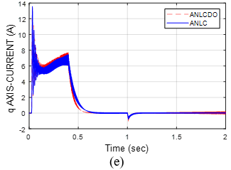
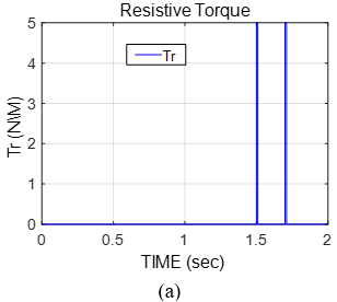
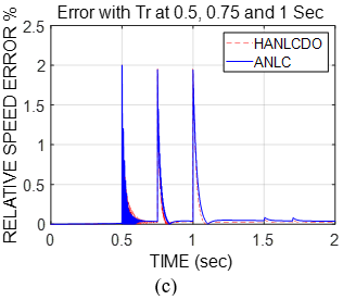
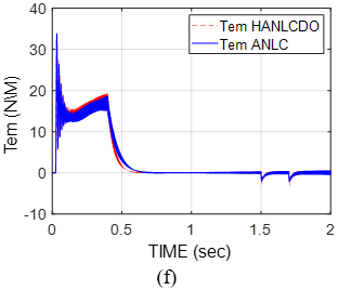
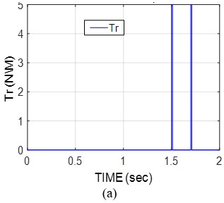
4.1.2 Scenario 2: Time-varying of (a form of a staircase) mechanical rotational speed with unknown load torque perturbation:
In this case, a time-varying mechanical rotational speed variation (in the form of a staircase) is considered while introducing an unknown load torque disturbance as Dirac impulses at 1.5 s and 1.7 s. This application of load torque as an impulse rather than a step is intended to rigorously test the robustness of the two control methods. Figure 4 illustrates the PMSM’s responses under mechanical rotational speed variation while considering unknown load torque disturbance. The results of Figure 4 and Table 2 demonstrate that the proposed control strategy achieves satisfactory tracking performance of $\omega_r$ and id while exhibiting high robustness against load torque disturbances. Particularly during the Dirac impulse application at times 1.5 s and 1.7 s. In addition, during these instances, the tracking performance of ωmexhibits a maximum relative error of approximately 0.1% and 0.07% with the ANLC and the suggested control scheme, respectively. As $\omega_r$ fluctuates, both the DO and ANLC methods consistently exhibit tracking performance, yielding identical maximum relative errors of approximately 2%, 1.8%, and 1.8% at times 0.5 s, 1 s, and 1.5 s, respectively. The comparison between the ANLC and the proposed method under this scenario highlights the effectiveness of the DO-based proposed control scheme in ensuring satisfactory performance and robustness versus load torque disturbances.
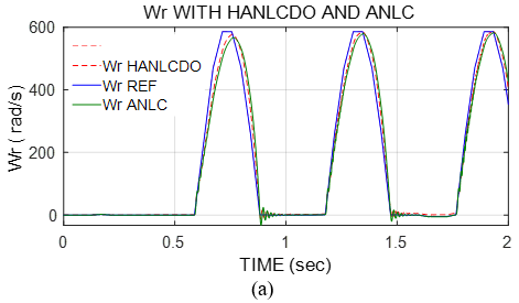
4.1.3 Scenario 3: Time-varying mechanical rotation speed without any perturbation in load torque:
This case study examines the effects of variation in mechanical speed, represented by a positive sine wave. This analysis aims to evaluate the control system's robustness against significant speed variations. As depicted in Figure 5 and Table 2, the relative error is measured at 1.18% and 0.82% for the ANLC and the proposed method, respectively. Notably, the proposed method consistently maintains a lower error compared to the ANLC.
4.2 Robustness to parameters variations Rs and Lq
This case study assesses the robustness of the proposed control scheme for three key parameters variations. In the first test, variation of the stator resistances (Rs) is considered, while the second and third cases adopt the inductance (Lq) and moment of inertia variation.
4.2.1 Case 1: Variation of the stator resistance Rs
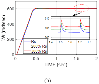
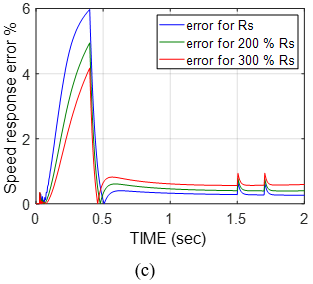
A test with three different values of the stator resistance, Rs, 2⨉Rs, and 3⨉Rs is conducted considering a load of 3N.m and unknown step-change load torque disturbance applied to the PMSM. Figure 6 displays the PMSM response to the three values of Rs, depicting the resistive torque (a), PMSM mechanical rotation speed (b), and speed relative error (c). From Figure 6(c), it can be observed that the peak relative error during the start phase for 100%, 200%, and 300% of Rs, are 6%, 5%, and 4.2%, respectively. Moreover, during steady-state operation, the relative errors do not exceed 0.8%. This indicates a high level of accuracy and stability in the control system, as evidenced by the near-zero speed response relative error even amidst variations in the stator resistance. Such robustness underscores the system's ability to maintain precise speed control despite fluctuations in stator resistance, highlighting its efficacy in real-world applications.
4.2.2 Case 2: Variation of the stator inductance Ls
Similarly, three different values of the inductance Lq are considered in this test also with applying a load of 3N.m to the PMSM. Figure 7 shows the PMSM system response to time-varying speed with load torque disturbances, emphasizing Lq variations, and it visualizes the same variables as the previous test. According to Figure 7(c), the peak relative errors during the start phase for different Lq variations, namely 100% Lq, 200% Lq, and 300% Lq, are about 6%, 7%, and 7.4%, respectively. Furthermore, during steady-state operation, the relative errors do not exceed 0.5%. The minimal speed response relative error observed during Lq variations underscores the system's resilience, accuracy, and stability, demonstrating its capability to uphold precise speed control despite changes in the inductance Lq.
4.2.3 Case 3: Variation of the moment of inertia J
Figure 8 demonstrates the speed response of the system using the proposed ANLCDO under different moment of inertia (J) values. The results show that the controller effectively tracks the reference speed with minimal deviation, ensuring robustness. Higher inertia (300% J) leads to slower acceleration and deceleration, enhancing stability but reducing responsiveness, while lower inertia (100% J) allows faster reactions but increases sensitivity to disturbances. Despite these differences, all responses accurately reach the reference speed, confirming the controller's adaptability and efficiency in maintaining stable and precise speed control across varying inertia conditions.
Figure 3. System response under a fixed mechanical speed and load torque with an unknown step-change; (a) load torque Tr, (b) mechanical rotational speed ωr, (c) relative speed error, (d)/(e) dq currents Idq, and (f) Electromechanical torque
Figure 4. System response under variable mechanical speed and load torque with an unknown step-change; (a) load torque Tr, (b) mechanical rotational speed ωr, (c) relative speed error, (d)/(e) dq currents Idq, and (f) Electromechanical torque
Figure 5. Responses for mechanical speed change without perturbation in load torque; (a) mechanical speed ωr and (b) relative speed error
Figure 6. Responses for three different values of stator resistance; (a) load torque Tr, (b) mechanical speed ωr, and (c) relative speed error
Figure 7. Simulation results for three different values of the inductance (a) mechanical speed ωr, and (b) relative speed error
Figure 8. Speed response with the proposed ANLCDO for three different values of the moment of inertia (J)
In this paper, an ANLC with a DO was proposed for regulating PMSMs within automotive electric propulsion systems. Our findings underscore the proposed method's effectiveness in ensuring robust and efficient control, even in the case of dynamic and nonlinear environments encountered in real-world applications. Through a series of simulation scenarios, we have demonstrated the superior performance of the suggested control approach compared to a conventional adaptive nonlinear control technique. In scenario 1, involving a gradually varying load torque disturbance, the proposed strategy exhibited significantly lower error rates and superior tracking performance of mechanical rotational speed (ωr) and stator current $\left(I_d\right)$ compared to ANLC. In addition, in scenario 2, where both load torque and mechanical speed changes were introduced, the proposed strategy consistently outperformed ANLC, maintaining stability and achieving satisfactory tracking performance even during critical instances of disturbance. Here, the proposed method consistently maintained lower error rates compared to ANLC, showcasing its ability to handle dynamic system changes effectively. The results further validate the efficacy of the developed controller in maintaining high accuracy and stability, with peak relative errors during the start phase not exceeding 7.4% and 7% for stator resistances and inductance variations, respectively, and the steady-state errors remaining below 0.8% and 0.5%, respectively. The integration of nonlinear adaptive control with a DO within the proposed method provides a promising solution to enhance the performance, stability, and robustness of automotive electric drive systems. These results provide valuable insights into the practical implementation of advanced control strategies and pave the way for further research and development in this area.
The study's limitations include reliance on simulation-based validation and specific PMSM parameters, which may not generalize to all motors. Future work should focus on experimental validation, enhancing adaptive algorithms, real-time implementation, and comprehensive disturbance testing. Additionally, comparative studies with other control techniques and integration with broader system components are recommended to ensure the robustness, adaptability, and practical applicability of the developed control approach in various real-world scenarios.
[1] Ni, R., Xu, D., Wang, G., Ding, L., Zhang, G., Qu, L. (2014). Maximum efficiency per ampere control of permanent-magnet synchronous machines. IEEE Transactions on Industrial Electronics, 62(4): 2135-2143. https://doi.org/10.1109/TIE.2014.2354238
[2] Zhu, Z.Q., Liang, D., Liu, K. (2021). Online parameter estimation for permanent magnet synchronous machines: An overview. IEEE Access, 9: 59059-59084. https://doi.org/10.1109/ACCESS.2021.3072959
[3] Eriksson, S. (2019). Permanent magnet synchronous machines. Energies, 12(14): 2830. https://doi.org/10.3390/en12142830
[4] F.F.M. El-Sousy, El-Sousy, F.F. (2012). Intelligent optimal recurrent wavelet Elman neural network control system for permanent-magnet synchronous motor servo drive. IEEE Transactions on Industrial Informatics, 9(4): 1986-2003. https://doi.org/10.1109/TII.2012.2230638
[5] Cheng, S., Li, C.W. (2011). Fuzzy PDFF-IIR controller for PMSM drive systems. Control Engineering Practice, 19(8): 828-835. https://doi.org/10.1016/j.conengprac.2011.04.011
[6] Mohanraj, D., Gopalakrishnan, J., Chokkalingam, B., Mihet-Popa, L. (2022). Critical aspects of electric motor drive controllers and mitigation of torque ripple. IEEE Access, 10: 73635-73674. https://doi.org/10.1109/ACCESS.2022.3187515
[7] Mesloub, H., Boumaaraf, R., Benchouia, M.T., Goléa, A., Goléa, N., Srairi, K. (2020). Comparative study of conventional DTC and DTC_SVM based control of PMSM motor—Simulation and experimental results. Mathematics and Computers in Simulation, 167: 296-307. https://doi.org/10.1016/j.matcom.2018.06.003
[8] Ma, Z., Saeidi, S., Kennel, R. (2014). FPGA implementation of model predictive control with constant switching frequency for PMSM drives. IEEE Transactions on Industrial Informatics, 10(4): 2055-2063. https://doi.org/10.1109/TII.2014.2344432
[9] Chai, S., Wang, L., Rogers, E. (2013). Model predictive control of a permanent magnet synchronous motor with experimental validation. Control Engineering Practice, 21(11): 1584-1593. https://doi.org/10.1016/j.conengprac.2013.07.008
[10] Liu, H., Li, S. (2011). Speed control for PMSM servo system using predictive functional control and extended state observer. IEEE Transactions on Industrial Electronics, 59(2): 1171-1183. https://doi.org/10.1109/TIE.2011.2162217
[11] Lee, T.S., Lin, C.H., Lin, F.J. (2005). An adaptive H∞ controller design for permanent magnet synchronous motor drives. Control Engineering Practice, 13(4): 425-439. https://doi.org/10.1016/j.conengprac.2004.04.001
[12] Luo, Y., Chen, Y., Ahn, H.S., Pi, Y. (2010). Fractional order robust control for cogging effect compensation in PMSM position servo systems: stability analysis and experiments. Control Engineering Practice, 18(9): 1022-1036. https://doi.org/10.1016/j.conengprac.2010.05.005
[13] Kim, S.K. (2017). Robust adaptive speed regulator with self-tuning law for surfaced-mounted permanent magnet synchronous motor. Control Engineering Practice, 61: 55-71. https://doi.org/10.1016/j.conengprac.2017.01.014
[14] Alsumiri, M., Li, L., Jiang, L., Tang, W. (2018). Residue theorem based soft sliding mode control for wind power generation systems. Protection and Control of Modern Power Systems, 3: 1-12. https://doi.org/10.1186/s41601-018-0097-x
[15] Leu, V.Q., Choi, H.H., Jung, J.W. (2011). Fuzzy sliding mode speed controller for PM synchronous motors with a load torque observer. IEEE Transactions on Power Electronics, 27(3): 1530-1539. https://doi.org/10.1109/TPEL.2011.2161488
[16] Kim, H., Son, J., Lee, J. (2010). A high-speed sliding-mode observer for the sensorless speed control of a PMSM. IEEE Transactions on Industrial Electronics, 58(9): 4069-4077. https://doi.org/10.1109/TIE.2010.2098357
[17] Hamida, M.A., De Leon, J., Glumineau, A. (2017). Experimental sensorless control for IPMSM by using integral backstepping strategy and adaptive high gain observer. Control Engineering Practice, 59: 64-76. https://doi.org/10.1016/j.conengprac.2016.11.012
[18] Kim, S.K., Lee, J.S., Lee, K.B. (2015). Offset-free robust adaptive back-stepping speed control for uncertain permanent magnet synchronous motor. IEEE Transactions on Power Electronics, 31(10): 7065-7076. https://doi.org/10.1109/TPEL.2015.2508041
[19] Morawiec, M. (2012). The adaptive backstepping control of permanent magnet synchronous motor supplied by current source inverter. IEEE Transactions on Industrial Informatics, 9(2): 1047-1055. https://doi.org/10.1109/TII.2012.2223478
[20] Bifaretti, S., Iacovone, V., Rocchi, A., Tomei, P., Verrelli, C.M. (2012). Nonlinear speed tracking control for sensorless PMSMs with unknown load torque: From theory to practice. Control Engineering Practice, 20(7): 714-724. https://doi.org/10.1016/j.conengprac.2012.03.010
[21] Verrelli, C.M., Tomei, P., Lorenzani, E., Migliazza, G., Immovilli, F. (2017). Nonlinear tracking control for sensorless permanent magnet synchronous motors with uncertainties. Control Engineering Practice, 60: 157-170. https://doi.org/10.1016/j.conengprac.2016.12.011
[22] Zhou, J., Wang, Y. (2005). Real-time nonlinear adaptive backstepping speed control for a PM synchronous motor. Control Engineering Practice, 13(10): 1259-1269. https://doi.org/10.1016/j.conengprac.2004.11.007
[23] Underwood, S.J., Husain, I. (2009). Online parameter estimation and adaptive control of permanent-magnet synchronous machines. IEEE Transactions on Industrial Electronics, 57(7): 2435-2443. https://doi.org/10.1109/TIE.2009.2036029
[24] Chaoui, H., Khayamy, M., Aljarboua, A.A. (2017). Adaptive interval type-2 fuzzy logic control for PMSM drives with a modified reference frame. IEEE Transactions on Industrial Electronics, 64(5): 3786-3797. https://doi.org/10.1109/TIE.2017.2650858
[25] Abu-Ali, M., Berkel, F., Manderla, M., Reimann, S., Kennel, R., Abdelrahem, M. (2022). Deep learning-based long-horizon MPC: Robust, high performing, and computationally efficient control for PMSM drives. IEEE Transactions on Power Electronics, 37(10): 12486-12501. https://doi.org/10.1109/TPEL.2022.3172681
[26] Song, Z., Yang, J., Mei, X., Tao, T., Xu, M. (2021). Deep reinforcement learning for permanent magnet synchronous motor speed control systems. Neural Computing and Applications, 33: 5409-5418. https://doi.org/10.1007/s00521-020-05352-1
[27] Fatemimoghadam, A., Iyer, L.V., Kar, N.C. (2024). Real-time validation of enhanced permanent magnet synchronous motor drive using dense-neural-network-based control. IEEE Access, 12: 73323-73339 https://doi.org/10.1109/ACCESS.2024.3403071
[28] Ullah, K., Guzinski, J., Mirza, A.F. (2022). Critical review on robust speed control techniques for permanent magnet synchronous motor (PMSM) speed regulation. Energies, 15(3): 1235. https://doi.org/10.3390/en15031235
[29] Wei, G.D., Qiang, Q.Z., Wei, Z., Zhi-Wu, K.Z., Yang, L. (2022). Intelligent decoupling control study of PMSM based on the neural network inverse system. Frontiers in Energy Research, 10: 936776. https://doi.org/10.3389/fenrg.2022.936776
[30] Solsona, J., Valla, M.I., Muravchik, C. (1996). A nonlinear reduced order observer for permanent magnet synchronous motors. IEEE Transactions on Industrial Electronics, 43(4): 492-497. https://doi.org/10.1109/41.510641
[31] Solsona, J., Valla, M.I., Muravchik, C. (2000). Nonlinear control of a permanent magnet synchronous motor with disturbance torque estimation. IEEE Transactions on Energy Conversion, 15(2): 163-168. https://doi.org/10.1109/60.866994
[32] Zhu, G., Dessaint, L.A., Akhrif, O., Kaddouri, A. (2000). Speed tracking control of a permanent-magnet synchronous motor with state and load torque observer. IEEE Transactions on Industrial Electronics, 47(2): 346-355. https://doi.org/10.1109/41.836350
[33] Kim, K.H., Youn, M.J. (2002). A nonlinear speed control for a PM synchronous motor using a simple disturbance estimation technique. IEEE Transactions on Industrial Electronics, 49(3): 524-535. https://doi.org/10.1109/TIE.2002.1005377
[34] Sira-Ramírez, H., Linares-Flores, J., García-Rodríguez, C., Contreras-Ordaz, M.A. (2014). On the control of the permanent magnet synchronous motor: An active disturbance rejection control approach. IEEE Transactions on Control Systems Technology, 22(5): 2056-2063. https://doi.org/10.1109/TCST.2014.2298238
[35] Linares-Flores, J., García-Rodríguez, C., Sira-Ramirez, H., Ramírez-Cárdenas, O.D. (2015). Robust backstepping tracking controller for low-speed PMSM positioning system: design, analysis, and implementation. IEEE Transactions on Industrial Informatics, 11(5): 1130-1141. https://doi.org/10.1109/TII.2015.2471814
[36] Preindl, M., Bolognani, S. (2013). Model predictive direct torque control with finite control set for PMSM drive systems, Part 1: Maximum torque per ampere operation. IEEE Transactions on Industrial Informatics, 9(4): 1912-1921. https://doi.org/10.1109/TII.2012.2227265
[37] Preindl, M., Bolognani, S. (2012). Model predictive direct torque control with finite control set for PMSM drive systems, part 2: Field weakening operation. IEEE Transactions on Industrial Informatics, 9(2): 648-657. https://doi.org/10.1109/TII.2012.2220353
[38] Niu, X., Zhang, C., Li, H. (2017). Active disturbance attenuation control for permanent magnet synchronous motor via feedback domination and disturbance observer. IET Control Theory & Applications, 11(6): 807-815. https://doi.org/10.1049/iet-cta.2016.1429
[39] Feng, Y., Yu, X., Han, F. (2012). High-order terminal sliding-mode observer for parameter estimation of a permanent-magnet synchronous motor. IEEE Transactions on industrial electronics, 60(10): 4272-4280. https://doi.org/10.1109/TIE.2012.2213561
[40] Liu, K., Zhu, Z.Q. (2013). Online estimation of the rotor flux linkage and voltage-source inverter nonlinearity in permanent magnet synchronous machine drives. IEEE Transactions on Power Electronics, 29(1): 418-427. https://doi.org/10.1109/TPEL.2013.2252024
[41] Yang, B., Yu, T., Shu, H., Dong, J., Jiang, L. (2018). Robust sliding-mode control of wind energy conversion systems for optimal power extraction via nonlinear perturbation observers. Applied Energy, 210: 711-723. https://doi.org/10.1016/j.apenergy.2017.08.027
[42] Zemmit, A., Messalti, S. (2016). Modeling and Simulation of Doubly Fed Induction Motor (DFIM) Control using DTC and DFOC: A comparative study. International Journal of Applied Engineering Research, 11(8): 5623-5628.
[43] Xu, W., Jiang, Y., Mu, C. (2016). Novel composite sliding mode control for PMSM drive system based on disturbance observer. IEEE Transactions on Applied Superconductivity, 26(7): 1-5. https://doi.org/10.1109/TASC.2016.2611623
[44] Zhang, X., Sun, L., Zhao, K., Sun, L. (2012). Nonlinear speed control for PMSM system using sliding-mode control and disturbance compensation techniques. IEEE Transactions on Power Electronics, 28(3): 1358-1365. https://doi.org/10.1109/TPEL.2012.2206610
[45] Li, S., Zhou, M., Yu, X. (2012). Design and implementation of terminal sliding mode control method for PMSM speed regulation system. IEEE Transactions on Industrial Informatics, 9(4): 1879-1891. https://doi.org/10.1109/TII.2012.2226896
[46] Tami, R., Boutat, D., Zheng, G., Kratz, F., El Gouri, R. (2017). Rotor speed, load torque and parameters estimations of a permanent magnet synchronous motor using extended observer forms. IET Control Theory & Applications, 11(9): 1485-1492. https://doi.org/10.1049/iet-cta.2016.0226
[47] Zhang, X., Li, Z. (2015). Sliding-mode observer-based mechanical parameter estimation for permanent magnet synchronous motor. IEEE Transactions on Power Electronics, 31(8): 5732-5745. https://doi.org/10.1109/TPEL.2015.2495183
[48] Son, Y.I., Kim, I.H., Choi, D.S., Shim, H. (2014). Robust cascade control of electric motor drives using dual reduced-order PI observer. IEEE Transactions on Industrial Electronics, 62(6): 3672-3682. https://doi.org/10.1109/TIE.2014.2374571
[49] Su, Y.X., Zheng, C.H., Duan, B.Y. (2005). Automatic disturbances rejection controller for precise motion control of permanent-magnet synchronous motors. IEEE Transactions on Industrial Electronics, 52(3): 814-823. https://doi.org/10.1109/TIE.2005.847583
[50] Jiang, Y., Xu, W., Mu, C., Liu, Y. (2017). Improved deadbeat predictive current control combined sliding mode strategy for PMSM drive system. IEEE Transactions on Vehicular Technology, 67(1): 251-263. https://doi.org/10.1109/TVT.2017.2752778
[51] Zhang, X., Hou, B., Mei, Y. (2016). Deadbeat predictive current control of permanent-magnet synchronous motors with stator current and disturbance observer. IEEE Transactions on Power Electronics, 32(5): 3818-3834. https://doi.org/10.1109/TPEL.2016.2592534
[52] Chen, J., Jiang, L., Yao, W., Wu, Q.H. (2014). Perturbation estimation based nonlinear adaptive control of a full-rated converter wind turbine for fault ride-through capability enhancement. IEEE Transactions on Power Systems, 29(6): 2733-2743. https://doi.org/10.1109/TPWRS.2014.2313813
[53] Jiang, L., Wu, Q.H., Wen, J.Y. (2004). Decentralized nonlinear adaptive control for multimachine power systems via high-gain perturbation observer. IEEE Transactions on Circuits and Systems I: Regular Papers, 51(10): 2052-2059. https://doi.org/10.1109/TCSI.2004.835657
[54] Hou, L., Ma, J., Wang, W. (2022). Sliding mode predictive current control of permanent magnet synchronous motor with cascaded variable rate sliding mode speed controller. IEEE Access, 10: 33992-34002. https://doi.org/10.1109/ACCESS.2022.3161629