Lendy Rahmadi*![]() | Hadiyanto
| Hadiyanto![]() | Ridwan Sanjaya
| Ridwan Sanjaya![]()
© 2025 The authors. This article is published by IIETA and is licensed under the CC BY 4.0 license (http://creativecommons.org/licenses/by/4.0/).
OPEN ACCESS
The goal of this study was to create a machine-learning model that could predict the growth patterns of hydroponically grown lettuce crops in the Nutrient Film Technique (NFT) system. To determine the best model for reliably and efficiently forecasting the growth patterns of lettuce crops, a comparison of four machine learning algorithm models was carried out. Four techniques were used to model machine learning: Support Vector Machines (SVM), K-Nearest Neighbors (K-NN), Random Forests (RF), and Gradient Boosting Classifiers (GB). The evaluation findings showed that the SVM algorithm had the lowest accuracy value of 80.5%, while the GB method was the most effective, with the greatest accuracy value of 93.4%. The K-NN algorithm's accuracy is 84.8%, whereas the RF method's is 90.4%. To increase the algorithm model's correctness, hyperparameter optimization was done. In addition to cross-validation, root mean square error (RMSE) measurements were conducted to determine the closest match between the observed data value and the model forecast.
machine learning, algorithm, lettuce grown pattern, hydroponics NFT systems
Hydroponics is becoming recognized as a feasible technique for fulfilling rising global food demand while reducing soil scarcity by 2050 [1]. Contemporary agricultural methods allow for the development of plants without soil by using a nutrient solution, leading in an increase in hydroponics practices [2]. However, certain factors influence plant growth in a hydroponic system. To achieve optimal growth in a hydroponic arrangement, these hydroponic variables must be recognized and handled in accordance with each plant's individual patterns.
Machine learning has been utilized in agriculture for a considerable duration. It improves the effectiveness and efficiency of several agricultural practices. It is employed to fulfill several agricultural needs, including data analysis, weather forecasting, plant selection suggestions, fertilizer assessment, disease identification in plants, and further uses [3]. Developing a high-performance prediction model through machine learning involves numerous challenges, such as choosing appropriate algorithms and ensuring that both the algorithms and the underlying platforms can handle large data quantities [4].
Several studies have applied machine learning to hydroponic agriculture, focusing on different predictive models and evaluation techniques. For example, Iniyan et al. [4] employed regression-based models to forecast crop yields, illustrating the efficacy of feature-engineering-based long short term memory (LSTM) with an accuracy of 86.3% [4]. Sulaiman et al. [1] examined predictions of phosphorus content utilizing Random Forests (RF), Support Vector Machines (SVM), and K-Nearest Neighbors (K-NN) classifiers, resulting in notable enhancements in precision [1]. However, most existing studies either focus on single machine learning models or apply limited feature selection techniques. Unlike these approaches, this study compares different classification models Gradient Boosting (GB), RF, SVM, and K-NN while also using hyperparameter adjustment to increase prediction accuracy. Furthermore, the dataset employed in this work is unusual in that it includes primary data from four harvest periods, resulting in high-resolution real-world application. These variables distinguish this study from earlier ones and add to the growing body of knowledge in the use of machine learning for hydroponic systems.
This study predicted the growth patterns of lettuce crops using machine learning. In order to assess the growth pattern, a classification strategy was utilized, which consisted of four different machine learning algorithms: GB, RF, K-NN and SVM.
The goal is to construct a model that can predict the growth of lettuce with high precision. Following the model's evaluation, a straightforward prediction test was run to determine how well the prediction model works in predicting the vegetable's growth pattern depending on the value of the entered variable. This model will assist in identifying the growth patterns of lettuce crops in hydroponic environments. This study evaluated the efficacy of four distinct machine learning algorithms in developing a robust predictive model.
The data included in the machine learning modelling comprises hydroponic plant growth variable data gathered from a site located at coordinates 4°00'32.9″ S, 103°14'48.1″ E, employing the NFT technology. There are three water storage reservoirs with varying capacities and nutrient profiles.
This research is novel due to its comparative evaluation of different machine learning models and its specific application to hydroponic NFT systems, utilizing a primary dataset gathered from four harvest cycles across three distinct growth patterns. Daily measurements were conducted, averaging eight data points per day, using calibrated instruments to ensure high precision. This high-resolution dataset, derived from real-world hydroponic systems, represents a unique and valuable contribution to the field, establishing a solid and pragmatic basis for the building and assessment of machine learning models intended for thorough plant growth monitoring.
Iniyan et al. [4] employed multiple regression models for crop yield estimation and found that the feature-engineering-based LSTM model exhibited the greatest efficiency, achieving an accuracy of 86.3% and yielding the lowest mean absolute error and root mean square error relative to other methods.
Sulaiman et al. [1] investigated the prediction of phosphorus concentrations in hydroponic solutions through the application of both individual and hybrid machine learning models. The prediction technique utilized three classification algorithms: SVM, RF, and K-NN.
Rahmadi et al. [3] conducted a study on crop prediction by amalgamating machine learning with the CRISP-DM approach, employing five distinct machine learning algorithms: Xtreme Gradient Boost (XGBoost), Decision Tree, Naïve Bayes, K-NN, and RF.
A novel methodology has been introduced to predict key physiological attributes of leaf lettuce (Lactuca sativa L.), including leaf count, leaf contour area, and dry mass. The investigation of the hydroponic system was conducted utilizing Artificial Intelligence (AI) approaches, encompassing fuzzy logic, neural networks, and a hybrid neural-fuzzy model [5].
Debroy and Seban [6] formulated two prediction models for forecasting tomato biomass in an aquaponics system utilizing an artificial neural network (ANN) and an adaptive neuro-fuzzy inference system (ANFIS), which combines ANN with fuzzy logic.
Abdullah et al. [7] introduced a prediction framework for examining the purchase behavior of online shoppers, employing several classification algorithms such as Decision Tree (DT), Multilayer Perceptron (MLP), XGBoost, SVM, and RF. The experimental findings indicate that the XGBoost classifier, which incorporates feature selection and oversampling techniques, demonstrated a significantly larger area under the curve.
Cedric et al. [8] developed a machine learning-based predictive method to estimate the national yield of rice, maize, cassava, seed cotton, yams, and bananas in West Africa throughout the year. Consolidated meteorological, climatic, agricultural, and chemical databases to assist policymakers and farmers in predicting annual crop yields at the national level. They developed a prediction system employing decision trees, multivariate logistic regression, and K-NN algorithms [8].
Another study used machine learning to examine farm-level wheat yield fluctuations using high-resolution satellite imaging, environmental, and topographical data. Using the scikit-learn machine learning framework, the forecasting procedure made use of regression models such as linear regression (LR), decision tree (DT), and RF. The training and validation of the models were conducted using over 10,000 data points sourced from 45 farms in the Fergana Valley, Central Asia [9].
Akhter and Sofi [10] examined the transformative role of emerging technologies such as Internet of Things (IoT), wireless sensor networks, data analytics, and machine learning in the context of smart agriculture. The study proposed an IoT-enabled predictive model for apple disease detection in the orchards of Kashmir using machine learning and conducted field surveys to assess technological awareness among farmers. The integration of these tools is shown to improve crop yield, monitor environmental conditions in real-time, and optimize decision-making in precision agriculture [10].
While high-resolution optical sensors have demonstrated promise in crop yield prediction, their broader application has been constrained by several challenges, including cloud interference, difficulties in identifying crop phenology, high computational demands, and the complexity of statistical modeling. As a result, the accuracy of yield predictions increased with the integration of these restored values into the regression analysis. Generalized Linear Regression (GLM) and RF are two baseline models that have shown better predictive ability than other ensemble and base models, as pointed out by Tesfaye et al. [11].
Four machine learning models XGB, RF, SVR, and Deep Neural Networks (DNN) were used in a 2022 study by Mokhtar et al. to forecast lettuce yield. The study examined three input variable combinations: dry weight, stem length, leaf count, water consumption, and stem diameter. Among the models, XGB, employing all input variables, attained the highest predictive accuracy, succeeded by SVR and RF. All models demonstrated robust predictive efficacy, with scatter index (SI) values consistently below 0.1 [12].
In 2023, Godwin Idoje et al. compared machine learning methods for four hydroponic system datasets: floating (FL), aggregate (AG), NFT, and aeroponic (AER). They utilized XGBoost, Federated Split Learning, Deep Neural Networks, and Linear Regression methodologies to forecast the width of garlic bulbs based on several factors, including days post-transplant, temperature, and nutrient composition. The results showed variations in algorithm performance with different R-squared and mean absolute errors values. The difference with this research lies in the focus on hydroponic systems and plant types. This research focuses on predicting the growth patterns of celandine crops using the NFT system and different algorithms for data modeling and analysis [13].
In this section, a detailed assessment of the essential literature on key concepts and theories connected to hydroponics, machine learning, techniques, and various machine learning algorithms is presented. The K-NN algorithm, the SVM algorithm, the RF algorithm, and the Boost Gradient Classifier algorithm are presented and discussed.
2.1 Machine learning
The field of computer science known as machine learning (ML) is a subfield that grants computers the ability to learn from data without the need for explicit programming. As a fundamental approach to Artificial Intelligence (AI), it enhances predictive accuracy by leveraging various features [11]. ML identifies patterns and correlations within data and extracts meaningful insights from datasets by training models based on prior experience [11].
When applied to the agricultural industry, machine learning has the potential to dramatically improve efficiency and simplify processes. This is accomplished by moving through three crucial stages: data collecting, model creation, and generalization procedures. Datasets that are typically complicated are typically processed and analyzed by machine learning algorithms [14]. Machine learning's main goal is to create computational algorithms that can use analytical or probabilistic models to extract predictive information from both static and dynamic data sources. These algorithms' performance is continuously improved through training and feedback.
2.2 Algorithm
The algorithms that are used in machine learning make predictions by studying and interpreting a variety of datasets, which may include test data or data that has not been investigated before. In the event that the accuracy that was achieved does not live up to the expectations, the algorithm is then subjected to larger datasets during which parameter modification can be utilized to improve its accuracy [3]. The process is repeated until the amount of accuracy that is required is achieved, at which point the algorithm is considered to have attained its maximum potential [3]. Based on how they learn, machine learning algorithms are generally separated into two major categories. The first category is supervised learning, which builds predictive models by classifying or predicting new, unseen data using labeled data. The second group is unsupervised learning, which finds patterns or hidden structures in unlabeled data, producing descriptive models [15]. Unlike traditional IT methods, machine learning techniques rely on a learning process that enables them to extract specific behaviours from data, making them highly effective in addressing various problems. Their flexibility and capability to enhance performance through data input make them useful tools in various fields [16].
2.2.1 Key Nearest Neighbors (K-NN)
The K-NN algorithm represents a straightforward and efficient approach utilized in instance-based learning, frequently employed in classification and regression tasks. It works by finding the closest data points within a specific feature space. By utilizing a specific distance measurement and preserving the training data, the K-NN approach finds these nearest neighbors [15]. In classification tasks, the K-NN algorithm determines the label of a new instance by analyzing the nearest k data points in the dataset. In regression, the estimation of a new instance's value is achieved through the calculation of a weighted ratio based on the values of its nearest neighbors [7].
The K-NN process involves a series of essential steps: (1) Distance Calculation, (2) Neighbor Selection, (3) Prediction Determination and (4) Assessment and Parameter Adjustment [17]. K-NN is well-known for being simple and easy to interpret, which makes it useful in many fields. However, its computational requirements can rise as the dataset becomes larger. K-NN still works well, though, in applications like pattern recognition, anomaly detection, and recommendation systems, providing a straightforward and adaptable answer to machine learning problems [18].
2.2.2 Support Vector Machine (SVM)
For issues involving regression and classification, a SVM is an effective learning algorithm. Its objective is to optimize a hyperplane, which serves as a boundary that separates data points into two categories [17]. SVM uses a hyperplane in a multidimensional space to categorize the data vectors. The maximal margin classifier, a fundamental variant of SVM, identifies the hyperplane that optimizes the margin when training data is linearly separable using binary classification [15].
To obtain an ideal hyperplane, the SVM determines the classification limits by optimizing support vectors, particularly near across classes [19]. Hyperplanes are chosen to maximize the distance to the nearest data points, referred to as support vectors. A fundamental term in SVM is the margin, defined as the minimum distance between the hyperplane and the nearest data points of each class. The SVM seeks to maximize this margin, as bigger margins signify improved generalization of previously unobserved data [20].
The SVM is a widely used mathematical formulation that aims to find a hyperplane with parameters w (weight vector) and b (bias) that minimizes the length of the weight vector. This optimization problem is the quadratic programming problem (QP). The goal is to ensure that the constraint $y_i\left(w \cdot x_i+b\right) \geq 1$ is satisfied for each data point $\left(x_i, y_i\right)$ in the training set [20].
2.2.3 Random Forest (RF)
RF is a prevalent and adaptable method in machine learning, recognized for its efficacy in classification and regression tasks. A decision tree partitions the data into smaller groupings according to the most significant features for predicting the target [21].
RF can easily handle classification and regression tasks on complex and large datasets. It deals with noise in the data and lost data and works well without requiring too many assumptions about the data distribution [20]. To construct a Rf model, multiple random decision trees are generated using a subset of the training data. Each tree is constructed utilizing a random selection of training features and data, operating independently from one another [21].
RF successfully address overfitting by merging predictions from numerous trees by majority voting or averaging. They can also provide feature importance scores, making them useful for feature selection, regression, and classification tasks [15]. The versatility, scalability, and outstanding performance of Rf render them a favored option for generating accurate and interpretable outcomes across various machine learning challenges [22].
2.2.4 Gradient Boost Classifier (GB)
The GB is an efficient machine learning method for solving classification and regression issues. Gradient boosting is a state of the art prediction technique that sequentially produces a model in the form of linear combinations of simple predictors typically decision trees by solving an infinite dimensional convex optimization problem [23].
The fundamental premise of the GB is to improve model performance by rectifying the flaws of prior predictions by the incorporation of new models that particularly address these residual errors. This iterative process continues until the prediction error reaches an acceptable threshold or the predefined number of iterations is completed [24]. The procedure commences with a preliminary weak classifier, followed by the computation of residuals, which denote the discrepancies between predicted and actual values. A novel weak classifier is subsequently trained on these residuals, and this process is reiterated until the residual errors are adequately minimized [25]. The GB algorithm utilizes a sequential ensemble methodology, commencing with a basic decision tree model featuring few splits and subsequently enhancing it by incorporating additional trees [26].
2.3 Confusion matrix
One machine learning method for evaluating the effectiveness of categorization models is the confusion matrix [20]. This facilitates the assessment of the model's accuracy in classifying things by juxtaposing its predictions with actual outcomes. The confusion matrix shows how many false positives, false negatives, and true positives there were [27]. Although the confusion matrix offers detailed information about model performance, using a single metric makes it easier to quickly compare the effectiveness of multiple classifiers [28]. Table 1 presents an illustration of a confusion matrix.
Table 1. Example of confusion matrix
|
Prediction |
Actual Value |
|
|
Positive |
TP |
FP |
|
Negative |
FN |
TN |
Evaluation metrics for binary classification frequently employ a confusion matrix for every model (refer to Table 1). The four primary components of the confusion matrix are false positives (FP), false negatives (FN), true positives (TP), and true negatives (TN). True positives refer to positive instances that have been accurately classified, whereas true negatives denote negative instances that have been correctly identified. False positives arise when negative instances are misclassified as positive, while false negatives occur when positive instances are misclassified as negative.
Based on Table 1, this study employed several performance metrics to evaluate model effectiveness [23]. Accuracy measures a classifier's overall correctness by evaluating the proportion of properly predicted outcomes to total predictions produced. It expresses how frequently the model produces right answers as the proportion of correctly classified instances among all evaluated instances. Accuracy values approaching 100% imply higher model reliability. The accuracy calculation formula is presented in the following Eq. (1):
Acuraccy $=\frac{T P+T N}{T P+T N+F P+F N}$ (1)
The ratio of accurately detected positive instances to all instances projected to be positive is known as precision. Perfect precision is indicated by a precision value of 1, which goes from 0 to 1. The formula used to calculate precision is presented in the following Eq. (2):
Precesion $=\frac{T P}{T P+F P}$ (2)
The percentage of accurately detected positive cases compared to all real positive instances is known as recall, sometimes called sensitivity or the True Positive Rate (TPR). The following equation contains the recall calculation formula (3):
Recall $=\frac{T P}{T P+F N}$ (3)
The F1 Score denotes the harmonic mean of Precision and Recall, so providing a balanced evaluation of these two metrics. The value ranges from 0 to 1, with rising scores indicating enhanced performance. The computation of the F1 Score is illustrated in the subsequent Eq. (4):
$F 1-$ Score $=\frac{2 *(\text { Precision } * \text { Recall })}{\text { Precision }+ \text { Recall }}$ (4)
2.4 Hydroponics
Hydroponics is an advantageous agricultural technique for cultivating fresh vegetables, particularly in regions with limited arable land or densely populated urban areas. In comparison with conventional soil-based agriculture, hydroponics provides a number of significant benefits, including more precise nutrient management, suitability for non-arable regions, efficient water and fertilizer usage, ease of sterilizing the growing medium at a low cost, and the ability to support high-density planting, which leads to greater yields per acre [29].
The ratio of the ideal value of the environmental indicator to the water content of hydroponic plants is related to the relationship between the growing environment and the content of water in hydroponic plants. The pH of the nutrient solution, nutrient content, ambient temperature, relative humidity, light intensity, and air CO2 are some crucial environmental indicators in hydroponics. The optimal value for each indicator must be evaluated in the appropriate ratio to guarantee that the plant's water content remains within ideal parameters [30].
Typically, plants absorb water and minerals from the soil; however, they still require these resources even when grown in soilless media. To comprehend plant interactions within hydroponic systems, it is essential first to understand the natural relationships plants have with the soil environment where they commonly thrive [29].
In planting using hydroponic systems, nutrient water quality is very important and should be considered. This example refers to the nutrient concentration (PPM = Part per million) used to calculate the concentration of a liquid solution [31]. Nutrient formulations are typically quantified in parts per million (ppm) for each vital component. One ppm indicates the presence of one unit of a specific substance per one million units of another substance [31].
Electrical conductivity (EC), or electrical conducting power, describes the heat concentration of dissolved nutrients in a solution. Each element has an electrical charge (cation to anode and anion to cathode), and the unit of measurement used to measure EC is mS/cm [32].
Total dissolved solids (TDS) are the water-soluble nutrient content of TDS, which determines the nutrients that the plant will absorb; therefore, it is necessary to monitor and maintain the nutrient content under ideal conditions for the plant. The amount of soluble substance compared to the solvent is called the solute concentration or known as the term part per million (ppm) with the unit mg/l, 1 ppm=1 mg/L,=1 gram/1,000 liters [32].
The pH scale quantifies the acidity of a solution. pH specifically measures the concentration of hydronium ions (H3O+). The scale operates logarithmically, extending from 0 to 14. The pH of pure water is 7.0. Water is considered acidic when the pH is below 7. The pH variable is significant as it influences the availability and absorption of certain essential atomic elements required for plant growth [32].
Each vegetable plant has different pH, EC, and TDS requirements, according to the characteristics of each vegetable. The water content can also be impacted by environmental elements as planting site, temperature, and humidity [33]. Table 2 presents the ideal TDS, EC, and pH values for different vegetable crops, guiding optimal nutrient management.
Table 2. TDS, EC and PH need for vegetables
|
Vegetable |
TDS (ppm) |
EC (mS/cm) |
pH Ideal |
|
Lettuce |
560-840 |
0,8-1,2 |
6,0-7,0 |
|
Lettuce Endive |
1.400-1.680 |
2,0-2,4 |
5,5 |
|
Lettuce Lororosa |
560-840 |
0,8-1,2 |
6,0-7,0 |
|
Water Lettuce |
560-840 |
0,8-1,2 |
6,0-7,0 |
|
Lettuce butterhead |
560-840 |
0,8-1,2 |
6,0-7,0 |
|
Celery |
1.260-1.680 |
1,8-2,4 |
6,5 |
However, nutritional development in plants also needs to consider the age of plant nutrition according to the plant age. The addition or increase in nutrient PPM is adjusted to the plant age, the older the plant life, and the higher the PPM required [30].
2.5 NFT systems
The NFT, a hydroponic specialty, was established in the late 1960s by Dr. A.J. Cooper of the Glasshouse Crops Research Institute in Littlehampton, England. It became commercially available in the early 1970s [34]. The NFT approach involves growing plants with their roots in a plastic film trough or rigid channel that continually circulates nutritional solution [35].
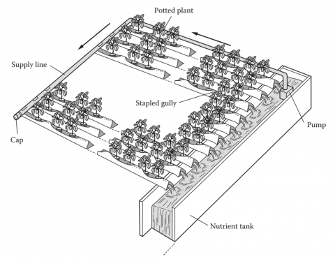
The fundamental principle of NFT is to nurture plants by enabling their roots to develop in a shallow, recirculating nutrient solution, which supplies adequate water, nutrients, and oxygen. Plants develop in polyethylene layers, with roots submerged in nutritional liquids that are perpetually cycled by a pump [36]. Figure 1 illustrates the fundamental principle of the NFT system, wherein a nutrient solution perpetually circulates via channels to facilitate plant growth.
Figure 1. NFT systems [29]
The basic workings of the NFT hydroponic system are depicted in Figure 1, where the nutrient solution travels via a main PVC pipeline to distribution headers that are placed at the top ends of the NFT channels. The solution is then poured into each planting channel or gully using short, flexible drip tubing. By gravity, the solution passes through the channels and empties into a catchment pipe at the bottom, which then returns it to the cistern. These channels are frequently set up on benches for simpler plant care and are used to cultivate low-profile crops [35].
2.6 Methodology
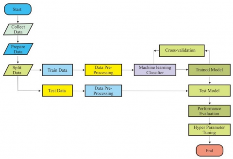
This section describes the research process, including data exploration, visualization, preprocessing, and machine learning model development. It explains the data used, the preparation techniques applied, and the evaluation of the methodology. Figure 2 offers a comprehensive graphic depiction of these stages.
Figure 2. Research stages
Figure 2 delineates the study phases, outlining the progression from data acquisition to model assessment.
2.7 Dataset description
The dataset used in this study is hydroponic NFT System variable experimental data for lettuce crops collected at the location coordinates 4°00'32.9″ "S 103°14'48.1"″ E.
Four hydroponic growth cycles, each 28 days from seedling to harvest, were studied. Eight preset time points every day measured environmental changes during the photoperiod. To document microenvironmental growth pattern alterations, high-frequency data collection was necessary.
Hydroponic systems need accurate sensors to collect high-quality data. Key environmental factors were measured precisely using various equipment. A Hygro Meter measured temperature and humidity with ±0.5℃ and ±3% RH precision, ensuring consistent climate tracking. The Lux Meter assessed light intensity with ±5% precision, enabling precise tracking of diurnal light exposure fluctuations. pH levels were measured with a Digital pH Meter, providing ±0.1 pH unit precision for reliable nutrition solution acidity tracking. Furthermore, an EC/TDS Meter accurately assessed Electrical Conductivity (EC) and Total Dissolved Solids (TDS) with ±2% precision, revealing nutrient concentration stability. These calibrated sensors kept environmental data correct for machine learning training.
Standard pH buffer solutions and known conductivity solutions for EC and TDS were used regularly to calibrate all sensors for dependability. Our strict calibration techniques are justified by prior studies linking incorrect calibration to model discrepancies [2].
Structured preprocessing was used to manage missing values, detect and eliminate outliers, and standardize feature scales to improve data quality and model accuracy. These steps improved the dataset for machine learning modeling.
The K-NN imputation approach was employed to estimate missing values since they made up less than 1% of the dataset [18]. Filling gaps with statistically meaningful values rather than eliminating useful data preserves data integrity. Outliers were found. Min-max normalization standardised values between 0 and 1 to ensure all variables contributed equally to the model. By preserving consistency across all input variables, this prevented bias from features with broader numerical ranges like EC and TDS and enhanced model performance. Preprocessing ensured a clean, balanced, and optimal dataset, improving machine learning predictions [11].
Values above 1.5 times the Interquartile Range (IQR) were considered abnormal and deleted. This phase was necessary to preserve model accuracy since excessive sensor values (e.g., EC and pH levels) could affect predictions.
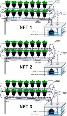
The data were collected using three hydroponic NFT systems used to plant and raise lettuce with three different patterns of enlargement and nutrition. Each NFT System consisted of two pipes with 40 plant holes. An illustration of the hydroponics of the NFT system used to collect data is shown in Figure 3.
Figure 3 illustrates the hydroponic NFT system, depicting the arrangement of plants within nutrient-enriched channels.
Figure 3. Hydroponics NFT system illustration
In this study, three patterns of plant enlargement and nutrition were used for lettuce in hydroponic NFT Systems. Each pattern is used in one hydroponic NFT system: the NFT 1 system is used for Pattern 1, the NFT 2 system is applied to Pattern 2, and the NFT 3 system for Pattern 3. Differences in lettuce enlargement and nutrition pattern for each pattern were found in the time and nutrition ratio within the reservoir of each NFT System. The differences between the enlargement and nutritional patterns of each pattern are shown in the following Table 3. Table 3 compares the three different growth patterns in the study, showing variations in nutrient concentration and pH levels over time.
Table 3. Patterrn comparison
|
Pattern |
Nutrition Day 1-7 (ppm) |
Nutrition Day 8-14 (ppm) |
Nutrition Day 15-21 (ppm) |
Nutrition Day 22-Harvest (ppm) |
pH |
EC mS/cm |
|
Pattern 1 |
400-500 |
400-500 |
800-1100 |
800-1100 |
6.0 – 7.0 |
800-2500 |
|
Pattern 2 |
100-200 |
300-400 |
500-600 |
700-840 |
6.0 - 7.0 |
300-1900 |
|
Pattern 3 |
600-800 |
600-800 |
1100-1400 |
1100-1400 |
6.0 – 7.0 |
1200-3000 |
These three patterns have different approaches to provide nutrition to lettuce crops in hydroponic NFT Systems. The first is a general growth pattern, which is a common choice in hydroponic farms. This pattern often follows general guidelines for providing plant nutrition without paying too much attention to specific nutrient ratio details. The second pattern is ideal, based on theory and references from various scientific journals and related books. This pattern emphasizes the importance of providing nutrients in the right proportions to suit the needs of plants at each growth stage. This approach has the potential to yield more optimal results in terms of growth, health, and productivity of hydroponic crops. The third pattern, known as the excess enlargement pattern, involves supplying nutrients in higher ratios and greater quantities compared to the first and second patterns. Although it can provide plants with more nutrients, this pattern can potentially lead to problems such as excess salt accumulation in the hydroponic system.
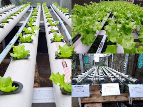
Figure 4 depicts the lettuce hydroponic NFT system used for data collection, including its structure and measurement setup.
Figure 4. Lettuce hydroponics NFT system to collect data
Figure 4 shows the NFT Hydroponic Illustration System deployment in Figure 3. There are six pipelines connecting to three reservoirs with hydroponics. Each hydroponic NFT system contains information about nutrient enlargement, plant types, and planting days. The collected data were assembled into a dataset and prepared for the next process. The dataset consists of 10 columns and 5005 rows before cleaning. All processes, including data collection, compilation, and data preparation, are one stage in data preparation.
3.1 Exploratory data analysis (EDA)
Conducting a thorough data analysis throughout the data-understanding step is critical to obtain the most accurate predictions for the processed dataset. An examination of the data's structure and descriptive qualities should be undertaken to achieve a comprehensive knowledge, employing diverse insights obtained from the dataset. In order to obtain a deeper understanding of the dataset and enable a more thorough assessment of its structure and properties, exploratory data analysis, or EDA, is carried out during the data understanding phase. To facilitate data comprehension, exploratory data analysis (EDA) provides insights into data descriptions, formats, and structures through various visual representations, including graphs, plots, descriptions, and maps [3].
Table 4 provides a statistical summary of numerical variables, including temperature, humidity, light, pH, EC, TDS, and water temperature.
Based on the statistics of data descriptions from the data frame in Table 4, we can obtain a variety of insights into the data used. The data had 10 attributes (before cleaning) and 5005 rows. The dataset contains 5005 unique data points for each attribute or variable temperature, humidity, light, pH, EC, TDS, and water temperature.
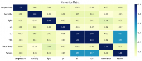
An illustration of the correlations between several variables in tabular form is called a correlation matrix. The correlation coefficient, which ranges from -1 to 1, signifies the degree and direction of the relationship between certain variables. For example, there is a high positive correlation between variables X and Y when the correlation coefficient value is 0.8. By analyzing the correlation matrix, patterns that may not be apparent when studying individual variables can be detected in the data. These patterns can provide additional insights into how variables interact with each other.
The quantity of cells in the correlation matrix aligned with the total count of variables in the dataset. For example, if there are five variables in the dataset, the correlation matrix has 25 cells (5 × 5). This makes it an efficient tool for exploring relationships among variables in complex datasets [37].
The correlation matrix can be visualized as a color matrix, displaying the correlation values using a color scale. This allows researchers to identify the correlation patterns in the dataset visually. The correlation matrix for the dataset is depicted in Figure 5 demonstrating the connections between important hydroponic parameters such as pH, TDS, and Electrical Conductivity (EC).
A correlation exists between Electrical Conductivity (EC) and Total Dissolved Solids (TDS). The lowest TDS value was recorded at a ratio of 161, while the lowest EC value was observed at a ratio of 336. In contrast, the highest TDS value was 1934 and the highest EC value was 3178. It is worth noting that the EC value is closely related to nutritional value because electrical conductivity has a strong positive relationship with the nutritional value, which is described by the total number of dissolved solids.
Figure 5. Correlation matrix
Figure 6. Boxplot each variable by pattern
Table 4. Statistic description of numerical variable
|
|
Temp |
Humidity |
Light |
pH |
EC |
TDS |
WaterTem |
|
count |
5005 |
5005 |
5005 |
5005 |
5005 |
5005 |
5005 |
|
mean |
28.9 |
76.7 |
34558.56 |
6.52 |
1675.3 |
837.8 |
26.2 |
|
std |
75.2 |
22.9 |
49156.29 |
0.26 |
728.3 |
364.7 |
2.3 |
|
min |
21.8 |
0 |
560 |
5.7 |
336 |
161 |
3.6 |
|
25% |
24.8 |
62 |
8300 |
6.4 |
1143 |
571 |
24.5 |
|
50% |
26.3 |
83 |
18840 |
6.5 |
1587 |
793 |
26.1 |
|
75% |
28.0 |
99 |
39420 |
6.7 |
2248 |
1124 |
27.5 |
|
max |
2619.0 |
99 |
70200 |
7.1 |
3178 |
1934 |
34.2 |
A boxplot is useful for graphically visualizing data distribution by showing key values, such as quarters, medians, and potential outliers. By utilizing boxplots, researchers can detect key patterns in hydroponic data, which serve as valuable insights for developing machine learning models [38]. Using a box plot, researchers can visually evaluate the distribution and comparison of hydroponic variables, which will provide valuable insights into the modeling of the growth of celery crops [39]. Figure 6 visualizes the distribution of each hydroponic variable using boxplots, comparing data variations across different growth patterns.
Figure 6 shows the visualization of patterns for each variable supplied in the box plot. The boxplot allows us to understand the range of values for each variable from lowest to highest based on the data used. By understanding the distribution and variation of hydroponic variables using a boxplot, we can select the most significant features to be included in the predictive model [33]. By understanding the distribution of data and patterns using a boxplot, researchers can develop a more accurate machine learning model for predicting plant growth, which, in turn, can improve efficiency and productivity in hydroponic cultivation [40].
The boxplot of each variable against a pattern shows a visualization of each variable value range against each pattern. EC variables and TDS variables have significant variable value ranges that differ from each pattern, it can be seen that pattern one and pattern 2 for EC variable and TDS have a value range that is not in a long row, but for the value range on pattern 3 has a distant value range. This indicates that in Pattern 3, there is a higher value ratio range than in Patterns 1 and 2. This describes the magnitude of the correlation between EC and TDD variables. For other variables, there was no overly distant range of values. The pH variable for each pattern has a different variable ratio because the nutrient concentration level in the water is also different. In pattern 3, the pH ratio values tended to be wider because in pattern 3, the nutrient concentration was much higher than in patterns 1 and 2.
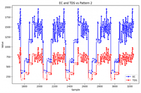
Each growth pattern had its variable movement, EC, and TDS. To determine the movement of variables TDS and EC for each pattern, we can see Figures 7 to 9 below. Figure 7 shows the fluctuation of EC and TDS values for Pattern 1, illustrating how nutrient levels change over time.
Figure 8 displays the movement of EC and TDS variables for Pattern 2, highlighting variations in nutrient concentration.
Figure 9 presents the fluctuation of EC and TDS in Pattern 3, indicating more extreme variations in nutrient concentrations.
Figure 7. Variable EC and TDS for pattern 1
Figure 8. Variable EC and TDS for pattern 2
Figure 9. Variable EC and TDS for pattern 3
Figure 7 shows the movement activity of the EC and TDS variables for Pattern 1. We can see that the value of TDS does not exceed 1000 ppm in pattern 1, and the EC value is not more than 2000 mS/cm. For Pattern 2, Figure 8 shows that the movement of the variables EC and TDS is wider and more variable. This is because the nutrition and enlargement of pattern 2 depend on the age of the plant, which is different from pattern 1. For Pattern 3's movement of the EC and TDS variables is shown in Figure 9. In Pattern 3, the ratio of the variable distance between EC and TDS was larger than that of Patterns 1 and 2. The maximum variable values for TDS are between 1200-1600 ppm with some highly variable leap points. The maximum EC values were between 2600 -3400 mS/cm.
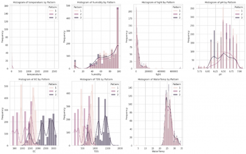
Figure 10. Histogram of each variable
A histogram was utilized to depict the study variables' frequency distribution. Histograms are one of the most commonly used techniques in statistical analysis to explore data distributions in various research fields, including agriculture. By identifying distribution patterns, such as a normal distribution or skewness, Researchers can get important knowledge that will help them choose the right characteristics and create machine learning models that are suitable for the task [41] .
Data visualization, particularly histograms, is a crucial component of data analysis as it facilitates the comprehension of variable interactions and the evaluation of model validity. By comparing the histogram of the actual data with the distribution predicted by the model, researchers can assess how well the model captures patterns in hydroponic data and identify potential areas for improvement to enhance its predictive accuracy [42]. Histograms have become an important tool for visually analyzing the distribution of hydroponic data. As a graphical method, histograms enable researchers to see data spreads clearly, thus facilitating an in-depth understanding of the datasets' characteristics [41]. Figure 10 provides histograms for each variable, helping to visualize the frequency distribution of hydroponic data.
From the histogram of each variable in Figure 10, we can perform a simple analysis to identify several things. The shape of the data frame consisted of 5005 and 10 columns. No missing values were in the data frame, and strong positive correlations were observed between the EC and TDS. Three patterns in the dataset were used, with details of pattern 1 having 1714 occurrences, pattern 2 having 1533 occurrences, and pattern 3 having 1758 occurrences. The dataset's key features are light, humidity, electrical conductivity (EC), water temperature, pH, total dissolved solids (TDS), and temperature because these elements are critical in determining plant growth. Monitoring and controlling these parameters can help establish optimal conditions for plant growth.
3.2 Preprocessing
Data preprocessing serves as a crucial phase in any data science endeavor, focused on refining and organizing the dataset to ensure its optimal application in predictive algorithms. This process ensures data consistency, enhances model accuracy, and improves overall analytical reliability [43]. Data preprocessing renders the dataset more consistent and structured, hence improving the overall performance of the generated model [44]. A significant problem in data the data's appropriateness for modeling, it is important to identify absent characteristics, pinpoint the impacted entries, and implement proper handling procedures according to the variable type. cleansing is the management of absent values. To guarantee This is important because the disappeared features may strongly predict the algorithm's outcome [43]. In building plant growth prediction models, the preprocessing stage, particularly data cleaning, is crucial for transforming raw data into usable data for the model. Data cleaning removes noise, outliers, and errors that could compromise the quality and accuracy of the predictive model, ensuring more reliable and effective analysis [28]. During data analysis and modeling, most of the time (80% or more) is devoted to data preparation such as loading, cleaning, transforming, and rearranging. Sometimes, the data are not in the correct format for a specific task because of the way they are stored in files or databases [45].
In the preprocessing phase of plant growth prediction models, data cleaning is a critical process for ensuring data quality. Data cleaning involves several steps such as handling missing values, detecting and removing outliers, data transformation, handling inconsistent data, and removing duplicate entries [26]. The initial step focused on identifying and addressing missing values within the dataset. This procedure can be completed by either eliminating rows or columns that include missing data or by using imputation techniques, which include substituting the mean, median, or mode of the available data for missing values [26].
In accordance with an 80:20 distribution ratio, the datasets were divided into two primary categories: training data and test data with 20% (1001 rows) set aside for testing and 80% (4004 rows) for training. For the purposes of this divide, eighty percent of the dataset was designated for training purposes, with the goal of assisting the model in learning patterns and relationships. The remaining twenty percent of the dataset was reserved for testing, with the intention of evaluating the model's performance and its capacity to generalize.
3.3 Modeling
In machine learning, the modeling stage is essential to creating models that can analyze intricate data patterns and generate precise predictions. Choosing a suitable model is essential for creating a successful machine learning system. Various factors, such as the data type, problem complexity, and accuracy requirements, should be considered when selecting a model [28]. Four machine learning methods were employed to create predictive models of vegetable development patterns: RF, SVM, K-NN, and GB.
The selection of machine learning algorithms is pivotal for attaining precise and dependable predictions of hydroponic lettuce growth patterns. This study employed K-NN, SVM, RF, and GB due to their efficacy in managing structured agricultural data, interpretability, and demonstrated success in hydroponic and agricultural modeling.
This necessitates machine learning algorithms capable of effectively capturing non-linear relationships and adapting to dynamic conditions [3]. Another critical aspect is feature importance and interpretability, as understanding which environmental factors have the most significant impact on plant growth is essential for optimizing hydroponic conditions and improving nutrient management strategies [2]. Considering these factors, the selection of machine learning algorithms was guided by their ability to manage complex data interactions, offer interpretability, and scale efficiently, ensuring robust and reliable predictions for hydroponic growth modeling.
In small-to-medium agricultural datasets, where pattern identification is essential, the distance-based method K-NN is frequently employed for classification tasks. This algorithm was chosen because of its capacity to handle missing values and noisy data, which are frequent problems in sensor-based datasets.
Additionally, K-NN performs well in identifying subtle variations in plant growth by analyzing environmental feature similarities, making it a suitable choice for hydroponic systems [46]. Another advantage of K-NN is its effectiveness in classifying lettuce growth stages, as it assigns labels based on the closest matching data points, allowing for accurate differentiation between various growth phases.
The SVM was chosen for its robust capacity to manage high-dimensional feature spaces and its efficacy in classifying non-linearly separable data. In hydroponic systems, where pH, electrical conductivity (EC), humidity, and nutrient concentrations interact in complex and dynamic ways, SVM provides robust generalization ability, making it particularly effective for small-to-moderate datasets [2].
Furthermore, by using kernel functions like the Radial Basis Function (RBF) to capture and describe non-linear interactions between environmental factors, SVM efficiently define distinct decision bounds for growth classification [1]. Another advantage of SVM is its ability to reduce overfitting, which is achieved by optimizing key hyperparameters such as C (regularization) and gamma, allowing the model to balance complexity and performance.
RF was selected for its robust performance in structured datasets with multiple interacting variables, making it particularly suitable for hydroponic growth prediction. A key advantage of RF is its capability to rank feature importance, enabling researchers to determine which environmental factors, such as pH, electrical conductivity (EC), and temperature, exert the most significant influence on lettuce growth [6].
GB was chosen as one of the most effective classification methods for structured datasets due to its strong predictive performance and ability to handle complex patterns, particularly for hydroponic sensor data, due to its iterative learning process that continuously refines predictions and minimizes errors over time. This approach enhances classification accuracy by allowing the model to learn from previous mistakes and make necessary adjustments in subsequent iterations.
GB is also well-suited for handling complex non-linear relationships, which is essential in hydroponic systems where variables such as electrical conductivity (EC), pH, and temperature interact in intricate ways that significantly influence plant growth. Unlike simpler models, GB has the advantage of adaptive error correction, enabling it to improve classification performance with each boosting cycle [3].
To validate our selection, Table 5 presents a comparative analysis of default and tuned accuracy scores is provided:
Table 5. Comparative analysis of default and tuned accuracy
|
Model |
Default Accuracy |
Tuned Accuracy |
Accuracy Gain |
|
K-NN |
79.9% |
84.8% |
+4.9% |
|
SVM |
75.8% |
80.5% |
+4.7% |
|
RF |
89.6% |
90.4% |
+0.8% |
|
GB |
92.2% |
93.4% |
+1.2% |
By combining these four models, this study ensures a comprehensive approach to hydroponic growth prediction, balancing accuracy, computational efficiency, and model interpretability to optimize decision-making in controlled agricultural environments.
Upon defining the machine learning model, it may be trained utilizing the specified training data. In this instance, 80% of the pre-divided entire dataset was employed for training. This approach entailed refining the model's parameters to discern patterns in the data. Model training is a crucial phase in machine learning, allowing models to learn and adjust proficiently to the provided dataset [47].
We divided the training model into two groups: hyperparameter tuning and without hyperparameter tuning. The initial group utilized default parameters to train the model, whereas the subsequent group investigated several hyperparameter setups to identify the optimal combination for enhanced model accuracy and performance. This split facilitates a precise assessment of the impact of hyperparameter tuning on the model's efficacy. Four distinct models Gradient Boosting Classifier, RF, SVM, and K-NN constitute a compendium of machine learning models, each associated with a certain classifier, facilitating quick access and comparison of various models. This approach provides flexibility for experimenting with various algorithms and facilitates exploring different model performance.
Once the model training process was completed, the subsequent step involved evaluating its performance using various assessment metrics. The confusion matrix is one of the most often utilized evaluation metrics.
This method is frequently utilized to evaluate classification models that forecast categorical event labels. The matrix is a grid that displays the true positives, false positives, true negatives, and false negatives that were produced during the testing phase [48].
3.4 Evaluation
Evaluation is an essential component of the modeling process, as it assesses the performance of the constructed model. Evaluation's main objective is to determine how well the model predicts observed data while making sure the outcomes align with the study's goals [44]. The assessment metrics described in this section are crucial markers for gauging the prediction accuracy of the model in classifying data. These metrics provide a comprehensive assessment of the alignment between the model's predictions and the data labels. Validation of an independent dataset is essential for an accurate evaluation of the model's performance.
To better understand model errors, we analyzed misclassified samples using the confusion matrix for each algorithm. K-NN struggled with distinguishing Pattern 2 and Pattern 3 due to overlapping nutrient concentrations, while SVM had difficulty separating Pattern 1 and Pattern 2 due to non-linearly separable data. RF misclassified some Pattern 3 samples, likely overfitting to extreme variations in electrical conductivity (EC) and total dissolved solids (TDS). Despite achieving the highest accuracy, GB still faced misclassification issues with borderline nutrient values, particularly between Pattern 2 and Pattern 3, indicating a need for further refinement in feature selection and dataset diversity.
Several factors contributed to these errors, including feature overlap, where similar environmental conditions (e.g., pH and temperature) made classification difficult, and sensor measurement variability, where slight inaccuracies in readings (e.g., ±10 ppm for TDS) introduced noise.
Table 6 presents more detailed evaluation and classification reports for each algorithm model. It summarizes the classification report for each algorithm, displaying precision, recall, and F1-score for different growth patterns.
Table 7 shows the Key Insights from Pattern-Based Performance Analysis.
Table 6. Classification report for each algorithm
|
PatertPatere Pattern |
Precision |
Recall |
F1-score |
Support |
||||||||||||
|
GB |
RF |
SVM |
K-NN |
GB |
RF |
SVM |
K-NN |
GB |
RF |
SVM |
K-NN |
GB |
RF |
SVM |
K-NN |
|
|
1 |
0.94 |
0.93 |
0.67 |
0.72 |
0.92 |
0.91 |
0.76 |
0.84 |
0.93 |
0.92 |
0.71 |
0.77 |
354 |
354 |
354 |
354 |
|
2 |
0.85 |
0.83 |
0.66 |
0.74 |
0.92 |
0.90 |
0.69 |
0.69 |
0.88 |
0.87 |
0.68 |
0.72 |
304 |
304 |
304 |
304 |
|
3 |
0.97 |
0.96 |
1.00 |
0.97 |
0.92 |
0.92 |
0.81 |
0.85 |
0.94 |
0.94 |
0.89 |
0.90 |
343 |
343 |
343 |
343 |
|
Macro Avg |
0.92 |
0.89 |
0.77 |
0.81 |
0.92 |
0.89 |
0.75 |
0.79 |
0.92 |
0.89 |
0.76 |
0.80 |
1001 |
1001 |
1001 |
1001 |
|
Weighted Avg |
0.92 |
0.89 |
0.78 |
0.81 |
0.92 |
0.89 |
0.76 |
0.80 |
0.92 |
0.89 |
0.76 |
0.80 |
1001 |
1001 |
1001 |
1001 |
|
Accuracy |
|
|
0.92 |
0.91 |
0.76 |
0.80 |
1001 |
1001 |
1001 |
1001 |
||||||
Table 7. Performance variation across growth patterns
|
Growth Pattern |
Best Performing Model |
Accuracy (%) |
Key Observations |
|
Pattern 1 (Standard Growth) |
Gradient Boosting |
94.2 |
Stable growth conditions led to high classification accuracy. |
|
Pattern 2 (Controlled pH & EC) |
Random Forest |
91.8 |
RF captured variability better under controlled conditions. |
|
Pattern 3 (Nutrient-Rich System) |
Gradient Boosting |
92.7 |
Excessive nutrient variation caused minor prediction inconsistencies. |
Model performance varied across the three hydroponic growth patterns, with GB and RF consistently achieving high accuracy. In Pattern 1 (General Growth Pattern), the GB model achieved the highest performance, with a precision of 0.94, a recall of 0.92, and an F1-score of 0.93, highlighting its effectiveness in predicting growth patterns, with most misclassifications occurring between Pattern 1 and Pattern 2 due to overlapping environmental factors like temperature and humidity. The superior performance of GB and RF suggests that ensemble methods work well in cases where feature similarities exist.
In Pattern 2 (Optimized Growth Pattern), the Gradient Boosting (GB) model once again outperformed the other models, achieving a precision of 0.85, a recall of 0.92, and an F1-score of 0.88, demonstrating its superior predictive performance, while SVM and K-NN struggled due to non-linear dependencies in the dataset. RF faced challenges distinguishing Pattern 2 from Pattern 3, likely due to variations in electrical conductivity (EC) and pH levels, which significantly impact nutrient absorption. This indicates that boosting techniques like GB adapt better to small nutrient ratio changes, while SVM and K-NN are less effective due to feature overlap.
In Pattern 3 (Excessive Nutrient Growth Pattern), GB showed the highest precision (0.97) and F1-score (0.94), while RF and SVM misclassified some samples as Pattern 2, likely due to extreme EC and TDS fluctuations. GB and RF were better suited for handling complex nutrient environments where feature distributions are skewed. Feature importance, hyperparameter sensitivity, and data overlap were identified as key factors influencing model performance, with GB excelling due to its iterative error correction capability.
GB consistently delivered the best performance, especially in Pattern 3, where variability was highest. RF was also effective but showed misclassification issues in Pattern 2 and 3, potentially due to overfitting. SVM and K-NN were less reliable in complex growth environments but acceptable for simpler cases like Pattern 1. These findings confirm that ensemble-based models, particularly GB, best suit hydroponic systems where environmental and nutrient conditions fluctuate significantly.
It is crucial to validate a model to ensure that it can perform well on data that has never been encountered before [49]. The Gradient Boosting (GB) approach utilizes a progressive ensemble of decision trees, commencing with the training of an initial weak tree characterized by minimum splits. Subsequently, fresh trees are incrementally introduced, each rectifying the faults of its predecessors, hence improving the overall model performance and predicted accuracy [26]. The RF method constructs multiple decision trees using tree-based algorithms, enhancing prediction accuracy through ensemble learning. In order to assess the importance of variables and ascertain how much they contribute to the predictive performance of the model, the Gini index is utilized [50].
The SVM is a versatile algorithm adept at managing many classification tasks, including those with high-dimensional data and nonlinear decision boundaries. However, one of its most significant drawbacks is that it requires precise adjustment of numerous hyperparameters in order to obtain optimal classification performance [51]. These hyperparameters include the kernel type, the regularization parameter, and the margin restrictions.
Table 8. Model comparison evaluation
|
Algortihm |
Accuracy |
Precision |
Recall |
F1-Score |
|
Gradient Boosting Classifier |
0.92 |
0.92 |
0.92 |
0.92 |
|
Random Forest |
0.89 |
0.89 |
0.89 |
0.89 |
|
Support Vector Machine |
0.76 |
0.77 |
0.75 |
0.76 |
|
K-Nearest Neighbors |
0.8 |
0.81 |
0.8 |
0.8 |
K-NN is an effective machine learning algorithm that can be utilized in multiple fields. Its key advantages include simplicity, interpretability, and ease of implementation. However, as dataset size grows, K-NN's computational complexity may become a limitation due to its reliance on distance calculations. Nonetheless, K-NN is exceptionally effective for anomaly detection, pattern identification, and recommendation systems, providing a versatile and intuitive methodology for addressing machine learning challenges [19].
To compare the evaluation results for each model, refer to Table 8. Table 8 presents a comparative analysis of model evaluation metrics, including accuracy, precision, recall, and F1-score, across various machine learning algorithms. This comparison provides insights into the effectiveness and reliability of each model in predicting outcomes.
The evaluation and validation of each machine learning algorithm were compared to assess their performance. The GB achieved the highest accuracy at 0.92, demonstrating its effectiveness in prediction. In contrast, the SVM exhibited the lowest accuracy, recording a score of 0.76. For more information on the difference between the training accuracy and the comparison for each model, please refer to Table 8. Table 9 presents training and test accuracy for each model, highlighting differences before and after hyperparameter tuning.
The RF model demonstrated the highest accuracy during training, achieving a precision score of 1.0. However, in contrast, the Gradient Boosting Classifier exhibited the best performance on the test dataset, indicating its superior generalization ability.
Table 9. Model evaluation accuracy
|
Model |
Train Accuracy |
Test Accuracy |
|
Gradient Boosting Classifier |
0.942308 |
0.919081 |
|
Random Forest |
1.000000 |
0.896104 |
|
Support Vector Machine |
0.766484 |
0.757243 |
|
K-Nearest Neighbors |
0.868132 |
0.799201 |
3.4.1 Hyper parameter tuning
Hyperparameter Tuning is a technique used to optimize parameters that the model cannot learn during training, process for creating effective systems [52]. Grid Search is a common method used for Hyperparameter Tuning, where we define a set of possible values for each hyperparameter and systematically combine them to find the best one. Random Search is another method in which we randomly select the values for each hyperparameter within a specified range. This approach is more efficient than the Grid Search for large parameter spaces [53]. To prevent overfitting, cross-validation was employed to fine-tune the hyperparameters and identify the optimal model configuration. This approach ensured that the model generalized well to unseen data by balancing bias and variance effectively [36].
Hyperparameter tuning was conducted in this study using Grid Search and Random Search to optimize machine learning models. Grid Search systematically tested predefined parameter combinations for each model, including n_neighbors and distance metrics for K-NN, kernel functions, C, and gamma values for SVM, n_estimators, max_depth, and split criteria for RF, and learning rate, n_estimators, and depth for Gradient Boosting. Since Grid Search is computationally intensive, Random Search was also applied to explore a broader parameter space efficiently. The best hyperparameters were selected using 5-fold cross-validation, with the final optimized parameters significantly improving model accuracy and reducing overfitting. This detailed tuning process enhances model reliability and facilitates replication by other researchers.
Table 10 demonstrate the impact of hyperparameter tuning, the following comparison was conducted between default settings and optimized models.
The results indicate that GB achieved the highest accuracy gain, whereas SVM and K-NN showed the most significant relative improvements due to the nature of their parameter sensitivity. These findings align with previous research indicating that boosting algorithms benefit most from hyperparameter tuning due to their iterative error correction mechanism [11].
Table 10. The comparison tuned accuracy
|
Model |
Default Accuracy |
Tuned Accuracy |
Accuracy Improvement |
|
Gradient Boosting |
92.2% |
93.4% |
+1.2% |
|
Random Forest |
89.6% |
90.4% |
+0.8% |
|
Support Vector Machine |
75.8% |
80.5% |
+4.7% |
|
K-Nearest Neighbors |
79.9% |
84.8% |
+4.9% |
Table 11. Model evaluation accuracy after fine-tuning
|
Model |
Train Accuracy |
Test Accuracy |
|
Gradient Boosting Classifier |
1.000000 |
0.934066 |
|
Random Forest |
1.000000 |
0.904096 |
|
Support Vector Machine |
0.842408 |
0.806194 |
|
K-Nearest Neighbors |
1.000000 |
0.848152 |
Hyperparameter tuning has demonstrated a notable increase in accuracy, precision, and recall, making models more robust for hydroponic system applications. However, it is worth noting that while Grid Search provides a systematic way to find optimal parameters, it is computationally expensive. Bayesian Optimization and Adaptive Hyperparameter Search could further improve efficiency by intelligently exploring parameter space rather than evaluating all combinations [53].
The dataset was randomly partitioned into multiple subsets, with one subset designated as the test set while the model was trained on the remaining subsets. This process was repeated iteratively, ensuring each subset served as the test set once, and the final model was derived by averaging the results from all iterations [36]. The data was split using an 80/20 ratio, where 80% was allocated for training and 20% for testing. Model fine-tuning was performed by adjusting hyperparameters to enhance accuracy. As demonstrated in Table 11, the accuracy of the machine learning algorithms improved following the tuning process. Table 11 lists the model accuracy after fine-tuning, showing improvements in GB, RF, SVM, and K-NN models.
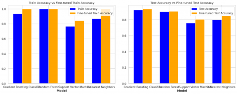
Figure 11 presents a detailed visualization of the combined accuracy results for all algorithms, enabling a comparison of model performance before and after hyperparameter tuning. This illustration highlights the improvements in prediction accuracy achieved through parameter optimization.
After fine-tuning the hyperparameters, the gradient boosting classifier improved testing accuracy. This suggests the optimization process led to a more effective model for the given task. The total change in accuracy was +1.2%, with an initial test accuracy of 92.2% and fine-tuned test accuracy of 93.4%. The RF model also showed a slight increase in testing accuracy after hyperparameter tuning, indicating that the optimization contributed to the enhanced model performance. The initial accuracy test results were 89.6%, which increased to 90.4% after fine-tuning, resulting in a change in accuracy of +0.8%.
Figure 11. Result accuracy comparison
Hyperparameter tuning significantly improved the SVM's testing accuracy, indicating that fine-tuned parameters led to a more accurate and effective model. The initial Test Accuracy score was 75.8%, which improved by +4.7% after fine-tuning to 80.5%. The K-NN model demonstrated the greatest increase in testing accuracy after hyperparameter tuning, with an accuracy increase of +4.9% from the initial accuracy test results of 79.9%–84.8% after fine-tuning.
This comparison emphasizes the role of hyperparameter tuning in improving the testing accuracy of machine learning models. It offers valuable insights into how parameter optimization influences overall model performance and effectiveness.
A simple deployment code prompt is created to test the growth pattern prediction model. The user enters values for specific features used in the machine-learning model, which are stored in a dictionary called input_values. Predictions are made using the transformed input values, and the code prints the prediction Table 11 showing the model names and their corresponding predictions based on the user input values.
In addition to performing cross validation during the evaluation phase, Root Mean Squared Error (RMSE) calculations were performed. The RMSE measures the model prediction's closeness to the observed data's actual value. The RMSE was determined by computing the square root of the mean squared difference between the actual and predicted values. The RMSE was computed using validation or test data that were independent of the training dataset. Lower RMSE values indicate better model performance, as they reflect higher accuracy in predicting previously unseen data. The RMSE results for all algorithms are presented in Table 12. Table 12 compares RMSE values before and after hyperparameter tuning, evaluating prediction error reduction across models.
Table 12. Evaluation use RMSE for each model
|
Model |
Without Hyperparameter Tuning |
With Hyperparameter Tuning |
||
|
RMSE Train |
RMSE Test |
RMSE Train |
RMSE Test |
|
|
Gradient Boosting Classifier |
0.104343 |
0.271978 |
0 |
0.286213 |
|
Random Forest |
0.288096 |
0.300735 |
0 |
0.369375 |
|
Support Vector Machine |
0.589781 |
0.617412 |
0.477255 |
0.527941 |
|
K-Nearest Neighbors |
0.362283 |
0.443895 |
0 |
0.466671 |
A model's performance can be enhanced by identifying the optimal set of hyperparameters through systematic tuning, which helps optimize accuracy and generalization. This helps us create a more accurate and reliable model to predict new data better. Tuning hyperparameters usually results in a lower RMSE value, indicating that the model is better at forecasting data. Table 12 shows the RMSE values for all the algorithm models used. It reveals that the lifting decreases are smaller for the entire model, especially for the Gradient Boost Classifier and RF. This suggests that tuning the hyperparameters leads to a more accurate data prediction.
A thorough assessment of machine learning models requires the integration of multiple performance metrics to effectively evaluate prediction accuracy, error magnitude, and overall model reliability. Although Root Mean Square Error (RMSE) is a widely used evaluation metric, relying exclusively on it may not fully capture a model’s overall performance. To overcome this limitation, incorporating additional metrics such as Mean Absolute Error (MAE) and the Coefficient of Determination (R²) is crucial for a more comprehensive assessment of model effectiveness, especially in predicting hydroponic lettuce growth patterns.
One of the primary limitations of RMSE is its sensitivity to large errors, as it penalizes extreme deviations more heavily than smaller ones. This characteristic makes RMSE particularly vulnerable to the influence of outliers, which can skew model evaluation and create a misleading impression of overall predictive performance [24]. Furthermore, RMSE alone does not provide insights into whether a model's predictions exhibit systematic bias or consistent overestimation or underestimation trends [54]. By incorporating Mean Absolute Error (MAE), which offers a clear measure of the average error magnitude without excessively emphasizing large deviations, along with R², which assesses the model's ability to explain variance in the target variable, a more comprehensive and balanced assessment of predictive accuracy can be attained. Table 13 below compares three key metrics:
Table 13. Three key metrics comparision
|
Model |
RMSE |
MAE |
R² |
|
Gradient Boosting |
0.286 |
0.142 |
0.92 |
|
Random Forest |
0.369 |
0.187 |
0.89 |
|
Support Vector Machine |
0.527 |
0.261 |
0.80 |
|
K-Nearest Neighbors |
0.466 |
0.232 |
0.84 |
The comparative evaluation of model performance highlighted several important insights into the effectiveness of various machine learning algorithms for predicting hydroponic lettuce growth patterns. Among the assessed models, Gradient Boosting (GB) exhibited the highest predictive accuracy, achieving the lowest RMSE (0.286) and the highest R² (0.92). This result confirms GB's superior capability in capturing complex, effectively capturing non-linear relationships within the dataset, establishing it as the most reliable model for predicting hydroponic growth. Additionally, the comparison of MAE and RMSE values across models showed that MAE values were consistently lower than RMSE, indicating that while extreme mispredictions existed, they were not dominant enough to significantly impact overall model performance. This suggests that the models performed well in general but may have had occasional outliers affecting RMSE more than MAE. Conversely, the SVM demonstrated the lowest predictive performance, recording an RMSE of 0.527 and an R² value of 0.80. This underperformance is likely attributed to SVM’s sensitivity to high-dimensional feature spaces and the lack of adequate kernel tuning, which may have prevented the model from effectively separating complex hydroponic growth patterns. These findings underscore the critical role of selecting appropriate machine learning techniques and fine-tuning model parameters to enhance predictive robustness and reliability in hydroponic systems.
3.4.2 Comparison with the existing works
This section compares the proposed algorithm model with similar studies conducted previously. Three studies were chosen for comparison: Sulaiman et al [1], Mokhtar et al. [12], Musleh et al. [16] , and Ahsain et al [55]. These studies were considered comparative because they used similar algorithm models. In a survey by Musleh et al. [16], the machine learning algorithms employed in this study included K-NN, SVM, RF, and GB. Among these, the SVM achieved the highest accuracy of 87% without the application of hyperparameter tuning. In comparison, the proposed model attained the highest accuracy of 93% using the Gradient Boosting Classifier following hyperparameter tuning. Sulaiman et al. [1] used multiple machine-learning algorithms, including the four used in this study. The Gradient Boost Classifier achieved the highest accuracy with an accuracy of 89% without performing hyperparameter tuning. Ahsain et al. [55] used an ensemble technique with the same three algorithms as the proposed model: K-NN, SVM, and RF. The highest accuracy (99.6 %) was achieved using the SVM algorithm.
Table 14 presents a comparison of the accuracy results obtained from the algorithm model used in the proposed study with those of previous work.
Table 14. Model evaluation accuracy after fine-tuning
|
Model |
Musleh et al. [1] Accuracy |
Ahsain et al. [52] Accuracy |
Sulaiman, et al. [1] Accuracy |
Mokhtar et al. [53] Accuracy (RMSE) |
This Study Accuracy |
|
Gradient Boosting Classifier |
82% |
89% |
- |
8.88g (XGBoost) |
93% |
|
Random Forest |
80% |
89% |
98% |
12.89g |
90% |
|
Support Vector Machine |
87% |
84% |
99% |
9.55 (Support Vector Regressor) |
80% |
|
K-Nearest Neighbors |
83% |
85% |
99% |
- |
84% |
As presented in Table 14, which summarizes the model evaluation accuracy after fine-tuning, Musleh et al. [16] found that the SVM algorithm was the most effective in their study, achieving a total accuracy of 87%. Similarly, Ahsain et al. [55] applied multiple algorithms, including four used in this study. They reported that the GB and RF models attained an accuracy of 89%. Meanwhile, Sulaiman et al. [55] did not employ the Gradient Boosting Classifier but instead utilized three similar algorithms. Their study leveraged ensemble learning techniques to develop hybrid predictive models, integrating techniques such as bootstrap aggregating (bagging), voting, and stacking. These ensemble methods were chosen for their effectiveness in improving model accuracy and reducing overfitting by combining predictions from multiple models. The ensemble approach demonstrated high accuracy, with the K-NN and SVM models attaining an accuracy rate of 99%. In the proposed study, among the four algorithm models used, the GB proved to be the most effective model following hyperparameter tuning, reaching an accuracy of 93%. Mokhtar [12] also conducted research on yield prediction for celery utilized four machine learning models: Deep Neural Networks (DNN), Xtreme Gradient Boosting (XGB), RF, and Support Vector Regressor (SVR). Their study collected harvest data from three hydroponic systems 50 days after planting over two years, using three scenarios that combined measured input variables. The key distinction between Mokhtar's study and the present research lies in the focus areas, collected datasets, and machine learning modelling methods. Regarding model evaluation, Mokhtar's study employed Root Mean Squared Error (RMSE), Mean Absolute Error (MAE), and R² as evaluation metrics to assess model performance, whereas the present study employed evaluation metrics, a confusion matrix, and RMSE. The results from Mokhtar's study indicated that in Scenario 3, The XGBoost (XGB) model yielded the lowest RMSE value of 8.88 g, followed by the Support Vector Regression (SVR) model with an RMSE of 9.55 g. In contrast, the RF model in Scenario 1 exhibited the highest RMSE value at 12.89 g.
Four machine learning methods were used in this study to estimate lettuce crop growth patterns in a NFT hydroponic system: GB, RF, K-NN and SVM. Hyperparameter tuning was performed to optimize model performance, significantly improving accuracy across all models. GB showed the highest improvement in testing accuracy, increasing from 92.2% to 93.4% (+1.2%), followed by R F, which improved from 89.6% to 90.4% (+0.8%). The SVM model showed a 4.7% increase from 75.8% to 80.5%, while K-NN achieved the highest improvement, rising from 79.9% to 84.8% (+4.9%). These findings underscore the significance of fine-tuning in improving predictive accuracy, thereby enhancing the reliability of the models for monitoring hydroponic crop growth.
The Root Mean Square Error (RMSE) was computed as a measure to evaluate the performance of the model, with lower values indicating higher prediction accuracy. Gradient Boosting (GB) had the lowest RMSE (0.286), confirming its strong predictive ability, followed by RF (0.369), K-NN (0.466), and SVM (0.527), which had the highest error. Additionally, comparisons with Mean Absolute Error (MAE) and R² scores provided a broader evaluation, The results indicate that Gradient Boosting (GB) demonstrated the highest overall performance, achieving an R² value of 0.937, while R F ranked second with an R² of 0.904. These findings suggest ensemble methods, particularly GB and RF, are more robust for handling complex hydroponic datasets.
Beyond model evaluation, the study's findings have practical applications in precision agriculture and smart hydroponic farming. The predictive models developed can be integrated into automated hydroponic monitoring systems, enabling farmers to optimize nutrient delivery, adjust environmental conditions, and improve crop yield predictions. Due to its superior performance, the GB model can be used in real-time hydroponic systems to detect early signs of suboptimal growth conditions, reducing waste and improving farming efficiency. Furthermore, understanding the relationships between nutrient levels and plant growth allows for more sustainable and cost-effective hydroponic practices.
Nevertheless, this study has certain limitations. The dataset was gathered from a single location with three nutrient patterns, which may restrict its generalizability. Future research should consider incorporating larger and more diverse datasets to enhance the robustness and applicability of the model. Additional features, such as CO₂ levels, root oxygenation, and nutrient uptake rates, could enhance prediction accuracy. Moreover, deep learning techniques like LSTM and CNNs could be explored for time-series forecasting, and real-world implementation through IoT-based monitoring systems would allow for continuous model refinement. Moving forward, integrating larger datasets, deep learning models, and real-time deployment strategies will be key to advancing machine learning applications in precision hydroponics.
We thank Lembah Dempo University and YPM Lembah Dempo for their support from various resources. The LD Media team conducted a plant-monitoring process to collect hydroponic data variables until harvest manually.
|
TP |
true positives |
|
TN |
true negatives |
|
FP |
false positives |
|
FN |
false negatives |
[1] Sulaiman, R., Azeman, N.H., Mokhtar, M.H.H., Mobarak, N.N., Abu Bakar, M.H., Bakar, A.A.A. (2024). Hybrid ensemble-based machine learning model for predicting phosphorus concentrations in hydroponic solution. Spectrochimica Acta Part A: Molecular and Biomolecular Spectroscopy, 304: 123327. https://doi.org/10.1016/j.saa.2023.123327
[2] Mehra, M., Saxena, S., Sankaranarayanan, S., Tom, R.J., Veeramanikandan, M. (2018). IoT based hydroponics system using Deep Neural Networks. Computers and Electronics in Agriculture, 155: 473-486. https://doi.org/10.1016/j.compag.2018.10.015
[3] Rahmadi, L., Hadiyanto, Sanjaya, R., Prambayun, A. (2023). Crop prediction using Machine Learning with CRISP-DM approach. In International Conference on Data Analytics & Management, pp. 399-421. https://doi.org/10.1007/978-981-99-6550-2_31
[4] Iniyan, S., Akhil Varma, V., Teja Naidu, C. (2023). Crop yield prediction using machine learning techniques. Advances in Engineering Software, 175: 103326. https://doi.org/10.1016/j.advengsoft.2022.103326
[5] Chang, C.L., Chung, S.C., Fu, W.L., Huang, C.C. (2021). Artificial intelligence approaches to predict growth, harvest day, and quality of lettuce (Lactuca sativa L.) in an IoT-enabled greenhouse system. Biosystems Engineering, 212: 77-105. https://doi.org/10.1016/j.biosystemseng.2021.09.015
[6] Debroy, P., Seban, L. (2022). A tomato fruit biomass prediction model for aquaponics system using machine learning algorithms. IFAC-PapersOnLine, 55(1): 709-714. https://doi.org/10.1016/j.ifacol.2022.04.116
[7] Khandokar, I.A., Islam, A.M., Islam, S., Shatabda, S. (2023). A gradient boosting classifier for purchase intention prediction of online shoppers. Heliyon, 9(4): e15163. https://doi.org/10.1016/j.heliyon.2023.e15163
[8] Cedric, L.S., Adoni, W.Y.H., Aworka, R., Zoueu, J.T., Mutombo, F.K., Krichen, M., Kimpolo, C.L.M. (2022). Crops yield prediction based on machine learning models: Case of West African countries. Smart Agricultural Technology, 2: 100049. https://doi.org/10.1016/j.atech.2022.100049
[9] Boori, M.S., Choudhary, K., Paringer, R., Kupriyanov, A. (2023). Machine learning for yield prediction in Fergana valley, Central Asia. Journal of the Saudi Society of Agricultural Sciences, 22(2): 107-120. https://doi.org/10.1016/j.jssas.2022.07.006
[10] Akhter, R., Sofi, S.A. (2022). Precision agriculture using IoT data analytics and machine learning. Journal of King Saud University-Computer and Information Sciences, 34(8): 5602-5618. https://doi.org/10.1016/j.jksuci.2021.05.013
[11] Tesfaye, A.A., Osgood, D., Aweke, B.G. (2021). Combining machine learning, space-time cloud restoration and phenology for farm-level wheat yield prediction. Artificial Intelligence in Agriculture, 5: 208-222. https://doi.org/10.1016/j.aiia.2021.10.002
[12] Mokhtar, A., El-Ssawy, W., He, H., Al-Anasari, N., Sammen, S.S., Gyasi-Agyei, Y., Abuarab, M. (2022). Using machine learning models to predict hydroponically grown lettuce yield. Frontiers in Plant Science, 13: 706042. https://doi.org/10.3389/fpls.2022.706042
[13] Idoje, G., Mouroutoglou, C., Dagiuklas, T., Kotsiras, A., Muddesar, I., Alefragkis, P. (2023). Comparative analysis of data using machine learning algorithms: A hydroponics system use case. Smart Agricultural Technology, 4: 100207. https://doi.org/10.1016/j.atech.2023.100207
[14] Van Klompenburg, T., Kassahun, A., Catal, C. (2020). Crop yield prediction using machine learning: A systematic literature review. Computers and Electronics in Agriculture, 177: 105709. https://doi.org/10.1016/j.compag.2020.105709
[15] Durai, S.K.S., Shamili, M.D. (2022). Smart farming using machine learning and deep learning techniques. Decision Analytics Journal, 3: 100041. https://doi.org/10.1016/j.dajour.2022.100041
[16] Musleh, D., Alkhwaja, A., Alkhwaja, I., Alghamdi, M., Abahussain, H., Albugami, M., Alfawaz, F., El-Ashker, S., Al-Hariri, M. (2024). Machine learning approaches for predicting risk of cardiometabolic disease among university students. Big Data and Cognitive Computing, 8(3): 31. https://doi.org/10.3390/ bdcc8030031
[17] Khennou, F., Fahim, C., Chaoui, H., Chaoui, N.E.H. (2019). A machine learning approach: Using predictive analytics to identify and analyze high risks patients with heart disease. International Journal of Machine Learning and Computing, 9(6): 762-767
[18] Hastie, T., Tibshirani, R., Friedman, J. (2009). The Elements of Statistical Learning: Data mining, Inference, and Prediction. New York: Springer. https://doi.org/10.1007/978-0-387-21606-5
[19] Guarneros-Nolasco, L.R., Cruz-Ramos, N.A., Alor-Hernández, G., Rodríguez-Mazahua, L., Sánchez-Cervantes, J.L. (2021). Identifying the main risk factors for cardiovascular diseases prediction using machine learning algorithms. Mathematics, 9(20): 2537. https://doi.org/10.3390/math9202537
[20] Bishop, C.M., Nasrabadi, N.M. (2006). Pattern Recognition and Machine Learning. New York: Springer.
[21] Müller, A.C., Guido, S. (2016). Introduction to Machine Learning with Python: A Guide for Data Scientists. O'Reilly Media, Inc
[22] Sun, W., Zhang, P., Wang, Z., Li, D. (2021). Prediction of cardiovascular diseases based on machine learning. ASP Transactions on Internet of Things, 1(1): 30-35.
[23] Bühlmann, P., Hothorn, T. (2007). Boosting algorithms: Regularization, prediction and model fitting. Statistical Science, 22(4): 477–505. https://doi.org/10.1214/07-STS242
[24] Friedman, J.H. (2001). Greedy function approximation: A gradient boosting machine. Annals of Statistics, 1189-1232. https://www.jstor.org/stable/2699986
[25] Reddy, B.S., Dhanasekhar, G., Likhitha, G., Hemalatha G., Sricharan, B. (2023). Phising website detection using machien learning. Journal of Emerging Technologies and Innovative Research, 10(4). https://www.jetir.org/view?paper=JETIR2304066.
[26] Natekin, A., Knoll, A. (2013). Gradient boosting machines, a tutorial. Frontiers in Neurorobotics, 7: 21. https://doi.org/10.3389/fnbot.2013.00021
[27] Gaye, B., Wulamu, A. (2019). Sentiment analysis of text classification algorithms using confusion matrix. In Cyberspace Data and Intelligence, and Cyber-Living, Syndrome, and Health: International 2019 Cyberspace Congress, CyberDI and CyberLife, Beijing, China, Proceedings, Part I, pp. 231-241. https://doi.org/10.1007/978-981-15-1922-2_16
[28] Aurélien, G. (2017). Hands-on machine learning with scikit-learn & tensorflow. Geron Aurelien, 134: 145-150.
[29] Resh, H.M. (2022). Hydroponic Food Production. CRC Press. https://doi.org/10.1201/9781003133254
[30] Singh, S.K., Singh, R. (2017). Hydroponics farming technology for vegetable production: A review. International Journal of Current Microbiology and Applied Sciences, 6(10): 3793-3813.
[31] Susilawati, S., Si, M. (2019). Dasar-Dasar Bertanam Secara Hidroponik. Kampus Unsri Palembang: Universitas Sriwijaya.
[32] Isnan, M. (2020). Hidroponik: Bertanam Sayuran Tanpa Tanah. AgroMedia.
[33] Tjendapati, C. (2017). Bertanam Sayuran Hidroponik Organik dengan Nutrisi Alami. AgroMedia.
[34] Gujarati, D.N. (2003). Basic Econometrics (Fourth Edition). McGraw-Hill.
[35] Spensley, K., Winsor, G.W., Cooper, A.J. (1978). Nutrient film technique-Crop culture in flowing nutrient solution. Outlook on Agriculture, 9(6): 299-305. https://doi.org/10.1177/003072707800900608
[36] Affan, M.F.F. (2004). High temperature effects on root absorption in hydroponic system. Doctoral dissertation, Master thesis, Kochi Unversity.
[37] Hair, J.F., Black, W.C., Babin, B.J., Anderson, R.E. (2010). Multivariate Data Analysis (Seventh Edition). Pearson Education
[38] Moore, D.S., McCabe, G.P., Craig, B.A. (2009). Introduction to the Practice of Statistics (Vol. 4). New York: WH Freeman.
[39] Nickerson, M.L., Venterea, R.T., Baker, J.M. (2018). Hidroponik: A primer. CRC Press.
[40] Wu, L., Lin, L., Cheng, Y. (2020). Sustainable and innovative agriculture: A case study on hydroponics. International Journal of Environmental Research and Public Health, 17(10): 3568.
[41] Manolakis, D., Ingle, V., Kogon, S. (2005). Statistical and Adaptive Signal Processing. Artech House Publishers.
[42] Flores-Contreras, E.A., Araújo, R.G., Rodríguez-Aguayo, A.A., Guzmán-Román, M., García-Venegas, J.C., Nájera-Martínez, E.F., Sosa-Hernández, J.E., Parra-Saldivar, R. (2023). Polysaccharides from the Sargassum and brown algae genus: Extraction, purification, and their potential therapeutic applications. Plants, 12(13): 2445. https://doi.org/10.3390/plants12132445
[43] Basu, K., Basu, T., Buckmire, R., Lal, N. (2019). Predictive models of student college commitment decisions using machine learning. Data, 4(2): 65. https://doi.org/10.3390/data4020065.
[44] Rahmadi, L., Sanjaya, R. (2024). Automated hydroponic growth simulation for lettuce using ARIMA and prophet models during rainy season in Indonesia. International Journal of Advanced Computer Science & Applications, 15(11): 37. http://doi.org/10.14569/IJACSA.2024.0151137
[45] McKinney, W. (2012). Python for data analysis: Data wrangling with Pandas, NumPy, and IPython. O'Reilly Media, Inc.
[46] Adidrana, D., Surantha, N. (2019). Hydroponic Nutrient Control System based on Internet of Things and K-Nearest Neighbors. In 2019 International Conference on Computer, Control, Informatics and its Applications (IC3INA), Tangerang, Indonesia, pp. 166-171. https://doi.org/10.1109/IC3INA48034.2019.8949585
[47] Goodfellow, I., Bengio, Y., Courville, A., Bengio, Y. (2016). Deep Learning (Vol. 1, No. 2). Cambridge: MIT Press.
[48] Saini, S.K., Chandel, G. (2023). Effective machine learning-based heart disease prediction model. In International Conference on Data Analytics & Management, pp. 169-180. https://doi.org/10.1007/978-981-99-6550-2_14
[49] Raschka, S., Mirjalili, V. (2019). Python Machine Learning: Machine Learning and Deep Learning with Python, scikit-learn, and TensorFlow 2 , Third Edition. Packt Publishing.
[50] EElavarasan, D., Vincent, D.R., Sharma, V., Zomaya, A.Y., Srinivasan, K. (2018). Forecasting yield by integrating agrarian factors and machine learning models: A survey. Computers and electronics in agriculture, 155: 257-282. https://doi.org/10.1016/j.compag.2018.10.024
[51] Soofi, A.A., Awan, A. (2017). Classification techniques in machine learning: Applications and issues. Journal of Basic & Applied Sciences, 13: 459-465.
[52] Chollet, F. (2018). Deep Learning with Python. Manning Publications Co.
[53] Li, L., Jamieson, K., DeSalvo, G., Rostamizadeh, A., Talwalkar, A. (2017). Hyperband: A novel bandit-based approach to hy-perparameter optimization. The Journal of Machine Learning Research, 18(1): 6765-6816
[54] Kratzert, F., Klotz, D., Herrnegger, M., Sampson, A.K., Hochreiter, S., Nearing, G.S. (2019). Toward improved predictions in ungauged basins: Exploiting the power of machine learning. Water Resources Research, 55(11): 11344–11354. https://doi.org/10.1029/2019WR026065
[55] Ahsain, S., Kbir, M.A. (2022). Predicting the client’s purchasing intention using Machine Learning models. In E3S Web of Conferences, 351: 01070. https://doi.org/10.1051/e3sconf/202235101070