Farazdaq R. Yaseen![]() | Mina Q. Kadhim*
| Mina Q. Kadhim*![]() | Huthaifa Al-Khazraji
| Huthaifa Al-Khazraji![]() | Amjad J. Humaidi
| Amjad J. Humaidi![]()
© 2024 The authors. This article is published by IIETA and is licensed under the CC BY 4.0 license (http://creativecommons.org/licenses/by/4.0/).
OPEN ACCESS
For improving the energy efficacy and control performance, integration of swarm optimization with controller design could successfully reach this objective. In this study, a comparative analysis has been conducted between two decentralized control structures based on optimized Proportional-Integral-Derivative (PID) and PID-Proportional (PID-P) controllers for optimal controlling of heating system in multi-zone building. Based on the energy balance equation, the mathematical dynamics model of the heating system is established in the building. In order to enhance and optimize the performances of both controllers, their design parameters are tuned based on Whale Optimization Algorithm (WOA). Two objectives have been considered in the optimization process of heating system. The first objective is to minimize the error in temperature, between the desired and real temperatures, based on IAE (Integral of Absolute Error) index, while the second objective is the minimization of the heat energy consumption. The normalization method has been used to adjust between the two differently-scaled objectives. Simulation results based on MATLAB reveal that the PID-P controller achieved better performance in terms of providing comfort indoor temperature with energy savings as compared to the PID controller.
heating system, energy consumption, control system, PID controller, swarm optimization techniques, whale optimization algorithm
The temperature in buildings is affected by the temperature of the surrounding area. Based on the thermal concept, heat is transferred from the high temperature area to the lower temperature area. For example, if the outside temperature of the building is colder than inside, the inside temperature of the building will tend to be colder [1]. There are many applications where the temperature needs to be set to a desire level while the outside temperature varies from below 0℃ to above 45℃ [2]. For example, the temperature in a poultry incubator must be adjusted right to fertilize the eggs during the incubation period [3]. Another example is the breeding of plants in a greenhouse. Temperature control of indoor greenhouses is necessary for growing crops to improve the quality of plants [4, 5]. On other hand, energy saving is also important to take into consideration while designing heating control system. In European countries, as an example, the buildings can make up about 40% of the total consumption of energy. Using intelligent controller for the heating system in the building, it can save up to 30% of the overall energy used [6]. Thus, the researchers' attention has been drawn to the developed and design of a control system that will ensure the balance between these two objectives. In this sense, the aim of this study is to design and optimize the controlled system which minimizing the cost of operating by reducing the energy consumption of the heater and meet a certain indoor desired temperature.
The use of feedback controller has been proven over the years as a good mechanism that could be used to improve the performance of systems from various fields [7-11]. In the context of control system design, the dynamic model of the system is a pre-requisition for development of control algorithm. As an example, the system model could be described by set of differential equations which describe the dynamic behavior of system. In this work, the development of mathematical dynamics model for the heating system of the building is established based on the energy balance equation.
In the literature, many classical and modern control schemes have been presented to control the heating system of building. For instance, Yadav and Gaur [2] presented a comparative study among different controllers to maintain a constant temperature in a room. These controllers are Internal Model Control (IMC), Fuzzy Logic Control (FLC), Model Reference Control (MRC) and Proportional-Integral-Derivative (PID). Bhushan et al. [12] evaluated and compared the performances of FLC (fuzzy logic control) and ANFIS (Adaptive Neuro-Fuzzy Inference System) to control the temperature within a specified period of time for water bath system. To maintain the room's temperature and reject disturbances originating from the outside temperature, Utama and Hari [1] proposed the PID Disturbance Observer (PID-DOB). The limitation of these works is that they consider a Single Input Single Output (SISO) heating system.
The considered building in this paper has two heaters and two rooms. The controlled system is Two Input-Two Output (TITO) system which is a challenging problem due to the interacting of process variables [13]. The dynamics of TITO systems may involve a potential variation in characteristics. Many control approaches have been developed and proposed for TITO systems. In spite of all advances controller, most of studies adopted the PID controller and its variants to control TITO systems due to its simplicity of design, reliability and implementation. However, to have improved dynamic performance of PID controller-based system, a suitable tuning method is required to find the best setting of gains for the terms of PID controller. To solve this problem, several studies have formulated the tuning process as an optimization problem. Then, optimization techniques are utilized to obtain the optimal design parameters of PID controller such as to reach optimal performance of controlled system [14]. Among different optimization methods, the bio-inspired optimization techniques have become popular to obtain optimal solution for many optimization problems such as tuning the PID controller [15-19]. Regardless that each of these studies enhances the tuning process of the PID controller, efforts to improve performance have continued.
The present work is aimed at combining the WOA with two decentralized control structures including PID and PID-P controllers to control and optimize the heating system performance. Most of the research in the field of process control consider single objective (i.e. the performance of the controller). In this paper, two objectives are included in the problem of performance optimization for the heating system; one objective includes minimization of heat energy consumption and the other is the minimization of IAE index, where the error is defined as the difference between the measured output and the target output of the temperature inside the building structure. As the two objectives are differently-scaled, the normalization method has been used to adjust the two objectives and obtained a well-converged solution.
The organization of this paper is prepared in six sections. The establishment of heating system dynamic model for multi-zone buildings has been presented in the next section. Section 2 presents the process for designing the two decentralized control structures. Section 4 explains the concept of the WOA. Section 5 reports and discusses the simulation findings of the heating system's performance with each decentralized control structure. Section 6 provides a summary of this paper's conclusion.
This section presents the mathematical dynamics model of the heating system in the building. The considered building in this paper has two rooms as shown in Figure 1.
Figure 1. Heating system of building
To maintain the temperature inside each room in a desired level, there is a heater in each room. The variation of the temperature in the outside of the building is considered as an external disturbance. Without loss of generality, there are some assumptions in the model have been made. It is assumed that the air in all the building is well-mixed. Accordingly, the air temperatures are assumed equal at different places of each room. Furthermore, no influence from humidity of the air, no influence from people in the building, and no influence from wind are made. Moreover, it is assumed that the indoor temperature is influence by one side of the outside temperature.
The energy balance equation in each room is given by [2]:
$\mathrm{q}_1-\mathrm{q}_{\mathrm{or} 1}=\mathrm{C}_{\mathrm{t} 1} \frac{\mathrm{dT}_1}{\mathrm{dt}}$ (1)
$\mathrm{q}_2-\mathrm{q}_{\mathrm{or} 2}=\mathrm{C}_{\mathrm{t} 2} \frac{\mathrm{dT}_2}{\mathrm{dt}}$ (2)
where, $q_1$ is the heat rate from the heater in the first room, $\mathrm{q}_{\text {or } 1}$ is the heat rate loss in the first room, $\mathrm{q}_2$ is the heat rate from the heater in the second room, $\mathrm{q}_{\text {or2 }}$ is the heat rate loss in the second room. The variables $T_1$ and $T_2$ represent the measured temperatures in the first and second room, respectively. $\mathrm{C}_{\mathrm{t} 1}$ and $\mathrm{C}_{\mathrm{t} 2}$ are air's thermal capacitance in each room. The thermal capacitance is given by [20]:
$C_t=m \cdot c$ (3)
where, the parameters $c$ and $m$ denote the specific heat and mass in the room, respectively. The heat rate loss in each room is given by:
$q_{\text {or } 1}=\frac{T_1-T_o}{R_{t 1}}+\frac{T_1-T_2}{R_{t 3}}$ (4)
$q_{\mathrm{or} 2}=\frac{\mathrm{T}_2-\mathrm{T}_{\mathrm{o}}}{\mathrm{R}_{\mathrm{t} 2}}+\frac{\mathrm{T}_2-\mathrm{T}_1}{\mathrm{R}_{\mathrm{t} 3}}$ (5)
where, $R_{t 1}$ is the wall thermal resistance between the first room and the outside, $R_{t 2}$ is the wall thermal resistance between the second room and the outside, $\mathrm{R}_{\mathrm{t} 3}$ is the wall thermal resistance between the two rooms. The wall thermal resistance is given by [20]:
$\mathrm{R}_{\mathrm{t}}=\frac{\mathrm{h}}{\mathrm{K}_{\mathrm{t}} \mathrm{A}}$ (6)
where, $h, K_t$ and $A$ represent the wall thickness, thermal conductivity of wall, and the area of wall, respectively. If Eq. (4) is substituted into Eq. (1) and Eq. (5) is substituted into Eq. (2) obtains:
$\mathrm{q}_1-\left(\frac{\mathrm{T}_1-\mathrm{T}_{\mathrm{o}}}{\mathrm{R}_{\mathrm{t} 1}}+\frac{\mathrm{T}_1-\mathrm{T}_2}{\mathrm{R}_{\mathrm{t} 3}}\right)=\mathrm{C}_{\mathrm{t} 1} \frac{\mathrm{dT}_1}{\mathrm{dt}}$ (7)
$\mathrm{q}_2-\left(\frac{\mathrm{T}_1-\mathrm{T}_{\mathrm{o}}}{\mathrm{R}_{\mathrm{t} 1}}+\frac{\mathrm{T}_1-\mathrm{T}_2}{\mathrm{R}_{\mathrm{t} 3}}\right)=\mathrm{C}_{\mathrm{t} 2} \frac{\mathrm{dT}_2}{\mathrm{dt}}$ (8)
Rearrange of Eq. (7) and Eq. (8) yields:
$\frac{\mathrm{dT}_1}{\mathrm{dt}}=-\left(\frac{\mathrm{T}_1-\mathrm{T}_{\mathrm{o}}}{\mathrm{C}_{\mathrm{t} 1} \mathrm{R}_{\mathrm{t} 1}}\right)-\left(\frac{\mathrm{T}_1-\mathrm{T}_2}{\mathrm{C}_{\mathrm{t} 1} \mathrm{R}_{\mathrm{t} 3}}\right)+\frac{1}{\mathrm{C}_{\mathrm{t} 1}} \mathrm{q}_1$ (9)
$\frac{\mathrm{dT}_2}{\mathrm{dt}}=-\left(\frac{\mathrm{T}_2-\mathrm{T}_{\mathrm{o}}}{\mathrm{C}_{\mathrm{t} 2} \mathrm{R}_{\mathrm{t} 2}}\right)-\left(\frac{\mathrm{T}_2-\mathrm{T}_1}{\mathrm{C}_{\mathrm{t} 2} \mathrm{R}_{\mathrm{t} 3}}\right)+\frac{1}{\mathrm{C}_{\mathrm{t} 2}} \mathrm{q}_2$ (10)
The control of the heating process involves addressing a range of issues and variables, including process control and the handling of uncertainties. While many reliable, sophisticated, and efficient controller systems have been developed, PID controllers have made a significant influence in the field of heating processes. Thus, two decentralized control approaches, represented by PID and PID-P controllers, are designed for temperature control in the building. The input to PID controller is the instantaneous error, which represents the difference between the measured (actual) output and desired (reference) setting of temperature [21]. Then, the PID controller results in summation of three control actions: proportional, summation of errors (integration) and rate of change of error (derivative) [22, 23]. Therefore, the control law based on PID control action can be described by [14]:
$U(s)=\left(K_p+\frac{K_i}{s}+\frac{K_d S}{K_t s+1}\right) E(s)$ (11)
where, $\mathrm{U}(\mathrm{s}), \mathrm{E}(\mathrm{s}), \mathrm{K}_{\mathrm{p}}, \mathrm{K}_{\mathrm{i}}, \mathrm{K}_{\mathrm{d}}$ and $\mathrm{K}_{\mathrm{t}}$ are the control law, the error, the proportional adjustable gain, the adjustable integral gain, the adjustable derivative gain and the derivative action time constant, respectively. The schematic structure of PID controller can be shown in Figure 2.
Figure 2. Schematic structure of PID controller
In addition to the three terms in the PID controller, the control law in the PID-P controller has another inner loop based on the weighed feedback gain $\mathrm{K}_{\mathrm{f}}$ of the output process $\mathrm{Y}(\mathrm{s})$. The control law of the PID-P controller is given by [24]:
$U(s)=\left(K_p+\frac{K_i}{s}+\frac{K_d s}{K_t s+1}\right) E(s)-K_f Y(s)$ (12)
Figure 3 shows the general block diagram of the PID-P controller.
Figure 3. The structure of PID-P control scheme
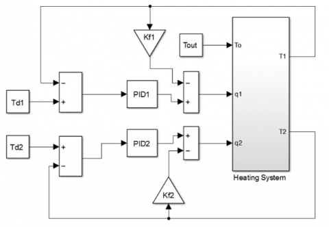
The two decentralized control structures as given in Figure 4 and Figure 5 are investigated to control the heating system of the building in this paper. Under each controller structure, the problem is to final the optimal value of the design variables of the controller in order to minimize heat energy consumption and minimize the error between the outputs and set-point. This problem is formulated as an optimization problem.
Figure 4. Decentralized PID control approach for TITO heating system
Figure 5. Decentralized PID-P controllers for TITO heating system
One class of algorithms that is applied to complex optimization problems is meta-heuristic optimization approaches. In contrast to traditional optimization techniques that depend on specialized knowledge for particular issues, meta-heuristics provide flexible, all-purpose approaches to problem-solving. These algorithms are developed based on the social interactions, natural occurrences, and different paradigms for addressing problems [18]. Mirjalili and Lewis [25] presented a meta-heuristic optimization algorithm called "Whale Optimization Algorithm (WOA)". The WOA is derived from studying humpback whale behavior and is made up of three sub-models: searching for a prey, feeding maneuver with spiral bubble-net, and encircling the prey. The pseudo-code of WOA is shown in Algorithm 1.
After humpback whales identify the position of prey (i.e. location of the best agent), they have two ways of moving around the prey simultaneously. The first way is the shrinking circle. In this mode, the humpback whales (i.e. other agents) update their positions on the way of best (search) agent. The following formulation is used for this purpose [25]:
$\mathrm{D}_{\mathrm{W}}=\left|\mathrm{C}_{\mathrm{W}} \mathrm{P}^*-\mathrm{P}_{\mathrm{i}}(\mathrm{itr})\right|$ (13)
$\mathrm{P}_{\mathrm{i}}(\mathrm{itr}+1)=\mathrm{P}^*-\left(\mathrm{A}_{\mathrm{W}} \mathrm{D}_{\mathrm{W}}\right)$ (14)
|
Algorithm 1: WOA's pseudo-code |
4. Print the Optimal Solution |
The coefficients $\mathrm{A}_{\mathrm{w}}$ and $\mathrm{C}_{\mathrm{w}}$ are computed as follows:
$\mathrm{A}_{\mathrm{w}}=2 \mathrm{a}_{\mathrm{w}} \mathrm{r}_1-\mathrm{a}_{\mathrm{w}}$ (15)
$C_w=2 r_2$ (16)
where, $i$, itr are the indices of agent and iteration, respectively. The parameters $P_i(i t r)$ and $P_i(i t r+1)$ represent the current and nest solution, respectively. The best solution is denoted by $\mathrm{P}^*$ and $\mathrm{a}_{\mathrm{w}}$ represents the coefficient, which is linearly decreased from value 2 to 0 . The coefficients $r_1, r_2$ are random values lying within the range [0.1]. The second way of moving is the spiral-shaped. In this mode, the movement of humpback whales is determined as follows [26]:
${{\overset{\acute{\ }}{\mathop{\text{D}}}\,}_{\text{w}}}=\left| {{\text{P}}^{\text{*}}}-\text{P}\left( \text{itr} \right) \right|$ (17)
${{\text{P}}_{\text{i}}}\left( \text{itr}+1 \right)={{\text{P}}^{\text{*}}}+\left( {{\overset{\acute{\ }}{\mathop{\text{D}}}\,}_{\text{w}}}{{\text{e}}^{{{\text{b}}_{\text{w}}}{{\text{l}}_{\text{w}}}}}\cos \left( 2\text{ }\!\!\pi\!\!\text{ }{{\text{l}}_{\text{w}}} \right) \right)$ (18)
where, the coefficient $\mathrm{b}_{\mathrm{w}}$ determine the shape of logarithmic spiral motion of whale and $\mathrm{l}_{\mathrm{w}}$ denoted a random number lying within a range [-1,1]. In order to maintain the right balance between the spiral mode and the shrinking encircling mode, it is assumed that there is a 50% chance to pick between the two modes. This mechanism can be formulated as follows [27]:
${{\text{P}}_{\text{i}}}\left( \text{itr}+1 \right)=\left\{ \begin{matrix} {{\text{P}}^{\text{*}}}-\left( {{\text{A}}_{\text{w}}}{{\text{D}}_{\text{w}}} \right)\rho >0.5 \\ {{\text{P}}^{\text{*}}}+\left( {{\overset{\acute{\ }}{\mathop{\text{D}}}\,}_{\text{w}}}{{\text{e}}^{{{\text{b}}_{\text{w}}}{{\text{l}}_{\text{w}}}}}\cos \left( 2\text{ }\!\!\pi\!\!\text{ }{{\text{l}}_{\text{w}}} \right) \right)~\rho \le 0.5 \\\end{matrix} \right.$ (19)
where, $\rho$ is also a random real number, which takes values between [0,1].
At the exploration stage, the humpback whales work randomly seeking for prey. Instead of using the best position of whale, the movement of each whale during this phase is dictated by the location of a randomly selected agent within the population. This behavior is performed when $\left|A_w\right| \geq 1$. The mathematical model of this process is given by:
$D_w=\left|C_w P_{\text {rand }}-P_i(t)\right|$ (20)
$P_i(t+1)=P_{\text {rand }}-\left(A_w \times D_w\right)$ (21)
where, $P_{\text {rand }}$ is a random position, which chosen from the individuals of population.
The experiment simulations of the controller design for the TITO heating system in the building using two decentralized control structures including PID and PID-P controllers are presented in this section. The numerical simulation of controlled heating system is implemented applying MATLAB programming software based on proposed controllers and the differential equations that are given in Eq. (9) and Eq. (10). Runge Kutta (ode45 in MATLAB) is utilized to simulate the differential equations. The system's parameters are listed in Table 1.
Table 1. The value of parameters of TITO heating system
|
Parameters |
Value |
|
Area of the Room1 $A_1$ |
16 $\mathrm{m}^2$ |
|
Area of the Room2 $A_2$ |
12 $\mathrm{m}^2$ |
|
Area between Rooms $A_3$ |
12 $\mathrm{m}^2$ |
|
Volume of the Room1 $V_1$ |
48 $\mathrm{m}^3$ |
|
Volume of the Room $V_2$ |
36 $\mathrm{m}^3$ |
|
Air Mass of the Room1 $m_1$ |
58.8 $\mathrm{K}_{\mathrm{g}}$ |
|
Air Mass of the Room2 $m_2$ |
44.1 $\mathrm{K}_{\mathrm{g}}$ |
|
Thickness of the Wall (h) |
0.2 m |
|
Thermal Conductivity Brick (K) |
1.43 $\mathrm{W}(\mathrm{mK})$ |
|
Air Density $(\rho)$ |
1.225 $\mathrm{K}_{\mathrm{g}} / \mathrm{m}^3$ |
|
Specific Heat of Air (c) |
1.005 $\mathrm{J} / \mathrm{K}_{\mathrm{g}} / \mathrm{K}$ |
Each heater's output power is limited by 0-5kw. Besides, it was assumed that the desired temperature in the first room is 30 Co while the desired temperature in the second room is 25 Co. The outside temperature is fixed at 0 Co. The simulation is run for one hour. The task of the optimized controller is to control and to minimize the cost of operation by reducing the energy consumption of each heater and to meet the indoor desired temperature. The design parameters of both PID and PID-P controllers are tuned by the WOA. The cost function of the optimization is built based on the two objectives.
In the first objective (CF1), the deviation between the desired and the actual of the output has to be minimized. The IAE (Integral of Absolute Errors) index that is used to evaluate the first objective [28].
$\mathrm{CF}_1=\mathrm{IAE}_1+\mathrm{IAE}_2$ (22)
$\mathrm{CF}_1=\int_{\mathrm{t}=0}^{\mathrm{t}=\mathrm{t}_{\text {sim }}}\left|\mathrm{e}_1(\mathrm{t})\right| \mathrm{dt}+\int_{\mathrm{t}=0}^{\mathrm{t}=\mathrm{t}_{\text {sim }}}\left|\mathrm{e}_2(\mathrm{t})\right| \mathrm{dt}$ (23)
where, $e_1(t)$ and $e_2(t)$ denote the errors between the desired and measured outputs in room 1 and room 2, respectively, and $\mathrm{t}_{\mathrm{sim}}$ refers to the time of the simulation.
The second objective ($\mathrm{CF}_2$) is to reduce the power consumption as given in Eq. (24) and Eq. (25).
$\mathrm{CF}_2=\mathrm{pc}_1+\mathrm{pc}_2$ (24)
$\mathrm{CF}_2=\int_{\mathrm{t}=0}^{\mathrm{t}=\mathrm{t}_{\operatorname{sim}}} \mathrm{u}_1(\mathrm{t}) \mathrm{dt}+\int_{\mathrm{t}=0}^{\mathrm{t}=\mathrm{t}_{\operatorname{sim}}} \mathrm{u}_2(\mathrm{t}) \mathrm{dt}$ (25)
where, $\mathrm{pc}_1(\mathrm{t})$ and $\mathrm{pc}_1(\mathrm{t})$ refer to the power consumption of the heaters in room1 and room 2 respectively. The normalization method as given in Eq. (26) has been used to adjust between the two differently-scaled objectives and determined the single cost function (CF) of the optimization [29, 30].
$\begin{aligned} & \mathrm{CF}=\omega_1\left(\frac{\mathrm{cf}_1-\min _{\mathrm{cf}_1}}{\max _{\mathrm{mf}_1}-\min _{\mathrm{cf}_1}}\right)+ \omega_2\left(\frac{\mathrm{cf}_2-\min _{\mathrm{cf}_2}}{\max _{\mathrm{cf}_2}-\min _{\mathrm{cf}_2}}\right)\end{aligned}$ (26)
where, $\omega_1$ and $\omega_2$ are used as a weight to justify between the two objectives. $\min _{\mathrm{cf}_1}$ and $\min _{\mathrm{cf}_1}$ are the estimated minimum values of each objective. $\max _{\mathrm{cf}_1}$ and $\max _{\mathrm{cf}_1}$ are the estimated maximum values of each objective. The WOA's parameters are listed in Table 2.
Table 2. The setting of WOA's parameters
|
Parameter |
Value |
|
No. of Iterations $\left(\mathrm{T}_{\max }\right)$ |
50 |
|
Size of Population $(\mathrm{N})$ |
50 |
The convergence of WOA for the two controller structures is shown in Figure 6. The optimal values of the designed parameters of two decentralized control structures, PID and PID-P controllers, are given in Table 3.
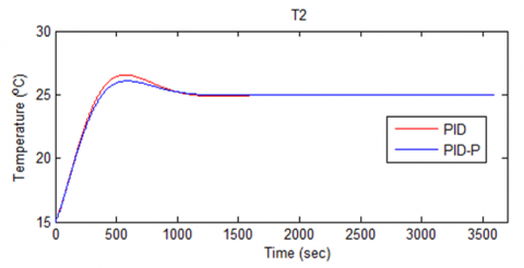
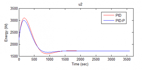
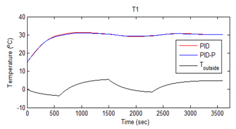
Figure 7 and Figure 8 show the response of the temperature in each room based proposed controllers. The behavior of power consumption inside room 1 and room 2 based on proposed controllers is illustrated in Figure 9 and Figure 10, respectively. It can be noticed based on Figure 9 and Figure 10 that the power consumption for both heaters based on the two control structures is within the acceptable range. The performance evaluation of proposed controllers is numerically reported in Table 4.
To evaluate the two control structures in terms of provide comfortable indoor temperature, it can be noticeable from Figure 7 and Figure 8 in addition to the second and third columns in Table 4 that the PID-P controllers are provided better comfortable indoor temperature in both rooms than the PID controllers. If the PID-P controllers are used, the IAE ${ }_1$ in the first room is 33832 and $\mathrm{IAE}_2$ in the second room is 22077 whereas if the PID controllers are used, IAE $_1$ in the first room is 35691 and the $\mathrm{IAE}_2$ in the second room is 23788.
In terms of power consumption, it can be observed based on Figure 9 and Figure 10 in addition fourth and fifth columns in Table 4 that the PID-P controllers are consumed less power consumption for both heaters than the PID controllers. If the PID-P controllers are used, the power consumption of the first heater is $142610\left(\frac{\mathrm{kw}}{\mathrm{h}}\right)$ and the power consumption of the second heater is $66713\left(\frac{\mathrm{kw}}{\mathrm{h}}\right)$ whereas if the PID controllers are used, the power consumption of the first heater is $142840\left(\frac{\mathrm{kw}}{\mathrm{h}}\right)$ and the power consumption of the second heater is $66918\left(\frac{\mathrm{kw}}{\mathrm{h}}\right)$.
Figure 6. Convergence of WOA for two controller structures
Table 3. Optimal value of each controller's adjustable parameters based on WOA
|
Controller |
Parameter |
Value |
|
PID |
$\mathrm{K}_{\mathrm{p} 1}$ |
250 |
|
$\mathrm{K}_{\mathrm{i} 1}$ |
1.3 |
|
|
$\mathrm{K}_{\mathrm{d} 1}$ |
0.2 |
|
|
$\mathrm{K}_{\mathrm{t} 1}$ |
10 |
|
|
$\mathrm{K}_{\mathrm{p} 2}$ |
220 |
|
|
$\mathrm{K}_{\mathrm{i} 2}$ |
1.6 |
|
|
$\mathrm{K}_{\mathrm{d} 2}$ |
0.2 |
|
|
$\mathrm{K}_{\mathrm{t} 2}$ |
5 |
|
|
PID-P |
$\mathrm{K}_{\mathrm{p} 1}$ |
296.5 |
|
$\mathrm{K}_{\mathrm{i} 1}$ |
1.52 |
|
|
$\mathrm{K}_{\mathrm{d} 1}$ |
0.26 |
|
|
$\mathrm{K}_{\mathrm{t} 1}$ |
7.25 |
|
|
$\mathrm{K}_{\mathrm{f} 1}$ |
32.5 |
|
|
$\mathrm{K}_{\mathrm{p} 1}$ |
246.87 |
|
|
$\mathrm{K}_{\mathrm{i} 1}$ |
1.7 |
|
|
$\mathrm{K}_{\mathrm{d} 1}$ |
0.14 |
|
|
$\mathrm{K}_{\mathrm{t} 1}$ |
9.67 |
|
|
$\mathrm{K}_{\mathrm{f} 1}$ |
19.6 |
Figure 7. Response of temperature of proposed controllers in the first room with fixed outside temperature
Figure 8. Behavior of temperature based on proposed controllers in the second room with fixed outside temperature
Figure 9. Power consumption of heater of proposed controllers in the first room with fixed outside temperature
Figure 10. Power consumption of heater of the proposed controllers in the second room with fixed outside temperature
Table 4. Performance metrics of proposed controllers with fixed outside temperature
|
Performance |
Value |
|
|
PID |
PID-P |
|
|
$\mathrm{IAE}_1$ |
35691 |
33832 |
|
$\mathrm{IAE}_2$ |
23788 |
22077 |
|
$\mathrm{pc}_1\left(\frac{\mathrm{kw}}{\mathrm{h}}\right)$ |
142840 |
142610 |
|
$\mathrm{pc}_2\left(\frac{\mathrm{kw}}{\mathrm{h}}\right)$ |
66918 |
66713 |
|
CF |
0.643 |
0.597 |
According to last column of Table 4, it has been shown that PID-P controller can results in CF equal to 0.597. However, this value of CF is lower than that based on PID controller, which is equal to 0.643. As such, the PID-P controller is achieved better performance in terms of providing comfort indoor temperature with energy savings as compared to the PID controller.
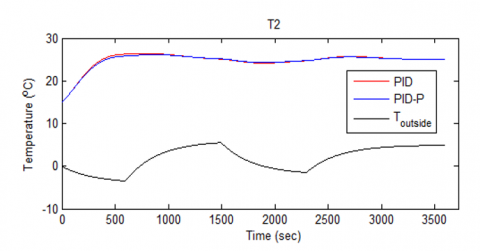
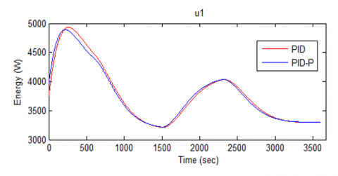
To evaluate the proposed controller in more realistic scenario, it is assumed that the outside temperature is varies from -4 to 6 Co during the simulation. Figure 11 and Figure 12 show the response of temperature in each room based proposed controllers. Besides, Figure 13 and Figure 14 illustrate the power consumption of the first and second room based proposed controllers. Figure 13 and Figure 14 show that, despite the fluctuating outdoor temperature, the power consumption for both heaters, based on the two control structures, is within the permitted range. The performance evaluation of the two controllers is given in Table 5.
Figure 11. Response of temperature of proposed controllers in the first room with varied outside temperature
Figure 12. Response of temperature of proposed controllers in the second room with varied outside temperature
Figure 13. Power consumption of heater of proposed controllers in the first room with varied outside temperature
Figure 14. Power consumption of heater of proposed controllers in the second room with varied outside temperature
Table 5. Performance metrics of proposed controllers with varied outside temperature
|
Performance |
Value |
|
|
PID |
PID-P |
|
|
$\mathrm{IAE}_1$ |
53550 |
49365 |
|
$\mathrm{IAE}_2$ |
35663 |
33284 |
|
$\mathrm{pc}_1\left(\frac{\mathrm{kw}}{\mathrm{h}}\right)$ |
136140 |
135790 |
|
$\mathrm{pc}_2\left(\frac{\mathrm{kw}}{\mathrm{h}}\right)$ |
61500 |
61328 |
|
CF |
0.985 |
0.90 |
Referring to Figure 11, Figure 12 and the third column in Table 5, one can deduce that the PID-P controller could achieve better comfortable indoor temperature in both rooms as compared to PID controllers under varying outside temperature. The IAE of the PID-P controllers in the first room is 49365 and in the second room is 33284 whereas the IAE of the PID controllers in the first room is 53550 and in the second room is 35663.
In terms of power consumption, it is evident from Figure 13, Figure 14 and Table 5 (fourth and fifth columns) that the PID-P controllers are consumed less power consumption for both heaters than the PID controllers. The power consumption of the PID-P controllers for the first heater is 135790 $\left(\frac{\mathrm{kw}}{\mathrm{h}}\right)$ and for the second heater is 61328 $\left(\frac{\mathrm{kw}}{\mathrm{h}}\right)$ whereas power consumption of the PID controllers for the first heater is 136140 $\left(\frac{\mathrm{kw}}{\mathrm{h}}\right)$ and for the second heater is 61500 $\left(\frac{\mathrm{kw}}{\mathrm{h}}\right)$ . According to Table 5 (last column), the value of CF in case of PID-P controller is equal to 0.90. However, this value of CF is lower than that using PID controller, which is equal to 0.985. As a result, the PID-P controller is achieved better performance in terms of providing comfort indoor temperature with energy savings as compared to the PID controller under varying outside temperature.
The aforementioned comparison of numerical results showed that an enhancement in performance of controlled heat system has been achieved by decentralized PID-P controllers as compared to the decentralized classical PID controllers of the heating control system has been achieved. Therefore, the decentralized PID-P controllers can be used to design a heating control system in multi-zone buildings to provide comfort indoor temperature with energy savings.
Controlling and optimization of proposed controller to improve the performance of heating system in multi-zone building are the objective of this study. This study took into consideration the influence of outdoor temperature. It also highlights the significance of control systems in achieving efficient and accurate temperature level by regulating heat rates. The differential equation of the heating system in the building is formulated based on the energy balance equation. The most popular method for controlling thermal processes is the classical PID controller, which has made significant advancements in the sector.
As the considered thermal system is TITO, two decentralized control structures including Proportional-Integral-Derivative (PID) and PID-Proportional (PID-P) controllers are proposed to achieve the best trade-off between minimizing energy consumption and meeting a certain indoor desired temperature. The problem of tuning the design variables of each control structure is formulated as an optimization problem. Then, a Whale Optimization Algorithm (WOA) has been proposed to optimize the adjustable parameters of both proposed control schemes. Besides, a normalization method has been used to adjust between the two differently-scaled objectives. Despite that, both control structures are able to stabilize the heating system based on the simulations results using MATLAB, but the control scheme using PID-P controller shows a good performance with regard to reduce the IAE index and provide comfortable indoor temperature with energy savings as compared to the PID controller.
|
$\mathrm{A}_1$ |
Area of the Room1 |
|
$\mathrm{A}_2$ |
Area of the Room2 |
|
$\mathrm{A}_3$ |
Area of the Room3 |
|
$\mathrm{a}_{\mathrm{w}}$ |
Coefficient linearly decreased from 2 to 0 |
|
$\mathrm{b}_{\mathrm{w}}$ |
Constant for defining the shape of the logarithmic spiral |
|
C |
Specific Heat of Air |
|
$\mathrm{C}_{\mathrm{t}}$ |
Thermal capacitance |
|
e, E(s) |
Error |
|
H |
Thickness of the Wall |
|
i |
Index of the agent |
|
itr |
Index of the iteration |
|
K |
Thermal Conductivity Brick |
|
$K_p$ |
Proportional gain |
|
$\mathrm{K}_{\mathrm{i}}$ |
Integral gain |
|
$K_d$ |
Derivative gain |
|
$K_t$ |
Derivative action time |
|
$\mathrm{l}_{\mathrm{W}}$ |
Random value between [-1,1] |
|
$\mathrm{m}_1$ |
Air Mass of the Room1 |
|
$\mathrm{~m}_2$ |
Air Mass of the Room2 |
|
N |
Population Size |
|
$\mathrm{P}^*$ |
Best solution |
|
$\mathrm{P}_{\mathrm{i}}(\mathrm{itr})$ |
Current solution |
|
$\mathrm{P}_{\mathrm{i}}(\mathrm{itr}+1)$ |
Next solution |
|
$\mathrm{P}_{\text {rand }}$ |
Random position chosen from the current population |
|
q |
Heat rate |
|
$\mathrm{R}_{\mathrm{t}}$ |
Thermal resistance |
|
$\mathrm{r}_1, \mathrm{r}_2$ |
Random value between [0,1] |
|
s |
Laplace operator |
|
$\mathrm{~T}_1$ |
Temperature in the first room |
|
$\mathrm{~T}_2$ |
Temperature in the second room |
|
$\mathrm{~T}_{\mathrm{d}}$ |
Desired temperature |
|
$\mathrm{T}_{\text {max }}$ |
Number of Iterations |
|
$\mathrm{T}_{\text {out }}$ |
Outside temperature |
|
$\mathrm{t}_{\text {sim }}$ |
Simulation time |
|
$\mathrm{u}, \mathrm{U}(\mathrm{s})$ |
Control law |
|
$V_1$ |
Volume of the Room1 |
|
$V_2$ |
Volume of the Room2 |
|
$\mathrm{Y}(\mathrm{s})$ |
Output of process |
|
Greek symbols |
|
|
$\rho$ |
Density of air |
|
$\omega_1, \omega_2$ |
Weights to justify between the two objectives |
|
Acronym |
|
|
ANFIS |
Adaptive Neuro-Fuzzy Inference System |
|
CF |
Cost function |
|
FLC |
Fuzzy Logic Control |
|
IAE |
Integral of Absolute Error |
|
IMC |
Internal Model Control |
|
MRC |
Model Reference Control |
|
PC |
Power consumption |
|
PID |
Proportional-Integral-Derivative |
|
PID-DOB |
PID Disturbance Observer |
|
PID-P |
PID-Proportional |
|
TITO |
Two Input Two Output |
|
WOA |
Whale Optimization Algorithm |
[1] Utama, Y.A.K., Hari, Y. (2017). Design of PID disturbance observer for temperature control on room heating system. In 2017 4th International Conference on Electrical Engineering, Computer Science and Informatics (EECSI), Yogyakarta, Indonesia, pp. 1-6. https://doi.org/10.1109/EECSI.2017.8239171
[2] Yadav, A.K., Gaur, P. (2013). Comparative analysis of modern control and AI-based control for maintaining constant ambient temperature. World Review of Science, Technology and Sustainable Development, 10(1-2-3): 56-77. https://doi.org/10.1504/WRSTSD.2013.050785
[3] Mumuni, F., Mumuni, A. (2015). Development of a state-space thermal model for high precision temperature control of a poultry incubator. IOSR Journal of Electrical and Electronics Engineering, 10(6): 52-57. https://doi.org/10.9790/1676-10625257
[4] Oubehar, H., Selmani, A., Ed-Dahhak, A., Archidi, M.H., Lachhab, A., Bouchikhi, B. (2020). Fuzzy-super twisting sliding mode for greenhouse climate control. In 2020 1st International Conference on Innovative Research in Applied Science, Engineering and Technology (IRASET), Meknes, Morocco, pp. 1-4. https://doi.org/10.1109/IRASET48871.2020.9092127
[5] Bennis, N., Duplaix, J., Enéa, G., Haloua, M., Youlal, H. (2008). Greenhouse climate modelling and robust control. Computers and Electronics in Agriculture, 61(2): 96-107. https://doi.org/10.1016/j.compag.2007.09.014
[6] Behravan, A., Obermaisser, R., Nasari, A. (2017). Thermal dynamic modeling and simulation of a heating system for a multi-zone office building equipped with demand controlled ventilation using MATLAB/Simulink. In 2017 International Conference on Circuits, System and Simulation (ICCSS), London, UK, pp. 103-108. https://doi.org/10.1109/CIRSYSSIM.2017.8023191
[7] Al-Khazraji, H., Cole, C., Guo, W. (2017). Dynamics analysis of a production-inventory control system with two pipelines feedback. Kybernetes, 46(10): 1632-1653. https://doi.org/10.1108/K-04-2017-0122
[8] Kadhim, M.Q., Hassan, M.Y. (2020). Design and optimization of backstepping controller applied to autonomous quadrotor. In IOP Conference Series: Materials Science and Engineering, p. 012128. https://doi.org/10.1088/1757-899X/881/1/012128
[9] Al-Khazraji, H., Naji, R.M., Khashan, M.K. (2024). Optimization of sliding mode and back-stepping controllers for AMB systems using gorilla troops algorithm. Journal Européen des Systèmes Automatisés, 57(2): 417-424. https://doi.org/10.18280/jesa.570211
[10] Ahmed, A.K., Al-Khazraji, H., Raafat, S.M. (2024). Optimized PI-PD control for varying time delay systems based on modified smith predictor. International Journal of Intelligent Engineering & Systems, 17(1): 331-342. https://doi.org/10.22266/ijies2024.0229.30
[11] Hamoudi, A.K., Rasheed, L.T. (2023). Design and implementation of adaptive backstepping control for position control of propeller-driven pendulum system. Journal Européen des Systèmes Automatisés, 56(2): 281-289. https://doi.org/10.18280/jesa.560213
[12] Bhushan, B., Sharma, A.K., Singh, D. (2016). Fuzzy & ANFIS based temperature control of water bath system. In 2016 IEEE 1st International Conference on Power Electronics, Intelligent Control and Energy Systems (ICPEICES), Delhi, India, pp. 1-6. https://doi.org/10.1109/ICPEICES.2016.7853729
[13] Lakshmanaprabu, S.K., Elhoseny, M., Shankar, K. (2019). Optimal tuning of decentralized fractional order PID controllers for TITO process using equivalent transfer function. Cognitive Systems Research, 58: 292-303. https://doi.org/10.1016/j.cogsys.2019.07.005
[14] Euzébio, T.A., Da Silva, M.T., Yamashita, A.S. (2021). Decentralized PID controller tuning based on nonlinear optimization to minimize the disturbance effects in coupled loops. IEEE Access, 9: 156857-156867. https://doi.org/10.1109/ACCESS.2021.3127795
[15] Chang, W.D. (2007). A multi-crossover genetic approach to multivariable PID controllers tuning. Expert Systems with Applications, 33(3): 620-626. https://doi.org/10.1016/j.eswa.2006.06.003
[16] Al-Khazraji, H., Khlil, S., Alabacy, Z. (2021). Cuckoo search optimization for solving product mix problem. In IOP Conference Series: Materials Science and Engineering, Baghdad, Iraq, p. 012016. https://doi.org/10.1088/1757-899X/1105/1/012016
[17] AL-Khazraji, H., Cole, C., Guo, W. (2021). Optimization and simulation of dynamic performance of production–inventory systems with multivariable controls. Mathematics, 9(5): 568. https://doi.org/10.3390/math9050568
[18] Al-Khazraji, H., Khlil, S., Alabacy, Z. (2020). Industrial picking and packing problem: Logistic management for products expedition. Journal of Mechanical Engineering Research and Developments, 43(2): 74-80.
[19] Mahmood, Z.N., Al-Khazraji, H., Mahdi, S.M. (2023). Adaptive control and enhanced algorithm for efficient drilling in composite materials. Journal Européen des Systèmes Automatisés, 56(3): 507-512. https://doi.org/10.18280/jesa.560319
[20] Burns, R. (2001). Advanced Control Engineering. Elsevier.
[21] Al-Khazraji, H., Cole, C., Guo, W. (2018). Analysing the impact of different classical controller strategies on the dynamics performance of production-inventory systems using state space approach. Journal of Modelling in Management, 13(1): 211-235. https://doi.org/10.1108/JM2-08-2016-0071
[22] Mahmood, Z.N., Al-Khazraji, H., Mahdi, S.M. (2023). PID-based enhanced flower pollination algorithm controller for drilling process in a composite material. Annales de Chimie Science des Matériaux, 47(2): 91-96. https://doi.org/10.18280/acsm.470205
[23] Ahmed, A.K., Al-Khazraji, H. (2023). Optimal control design for propeller pendulum systems using gorilla troops optimization. Journal Européen des Systèmes Automatisés, 56(4): 575-582. https://doi.org/10.18280/jesa.560407
[24] Gupta, R., Padhy, P.K. (2013). Design of PID-P controller for non-linear system using PSO. In 2013 Nirma University International Conference on Engineering (NUiCONE), Ahmedabad, India, pp. 1-6. https://doi.org/10.1109/NUiCONE.2013.6780184
[25] Mirjalili, S., Lewis, A. (2016). The whale optimization algorithm. Advances in Engineering Software, 95: 51-67. https://doi.org/10.1016/j.advengsoft.2016.01.008
[26] Al-Khazraji, H. (2022). Comparative study of whale optimization algorithm and flower pollination algorithm to solve workers assignment problem. International Journal of Production Management and Engineering, 10(1): 91-98. https://doi.org/10.4995/ijpme.2022.16736
[27] Patel, N.C., Debnath, M.K. (2019). Whale optimization algorithm tuned fuzzy integrated PI controller for LFC problem in thermal-hydro-wind interconnected system. In Applications of Computing, Automation and Wireless Systems in Electrical Engineering: Proceedings of MARC 2018, Singapore, pp. 67-77. https://doi.org/10.1007/978-981-13-6772-4_7
[28] Al-Khazraji, H., Cole, C., Guo, W. (2018). Multi-objective particle swarm optimisation approach for production-inventory control systems. Journal of Modelling in Management, 13(4): 1037-1056. https://doi.org/10.1108/JM2-02-2018-0027
[29] He, L., Ishibuchi, H., Trivedi, A., Wang, H., Nan, Y., Srinivasan, D. (2021). A survey of normalization methods in multiobjective evolutionary algorithms. IEEE Transactions on Evolutionary Computation, 25(6): 1028-1048. https://doi.org/10.1109/TEVC.2021.3076514
[30] Ishibuchi, H., Doi, K., Nojima, Y. (2017). On the effect of normalization in MOEA/D for multi-objective and many-objective optimization. Complex & Intelligent Systems, 3(4): 279-294. https://doi.org/10.1007/s40747-017-0061-9