Nawfal Berbiche*![]() | Mouna Chakir
| Mouna Chakir![]() | Mustapha Hlyal
| Mustapha Hlyal![]() | Jamila El Alami
| Jamila El Alami![]()
© 2024 The authors. This article is published by IIETA and is licensed under the CC BY 4.0 license (http://creativecommons.org/licenses/by/4.0/).
OPEN ACCESS
Confronted with budgetary constraints and complex sustainment systems in challenging environments, optimization of supply chains has become a necessity. The paper investigates a large body of literature related to integrated and decomposed supply chain problems’ modeling, optimization software and mathematical programming, including analytical and heuristic solution methods. The main purpose of this study is to contribute with a review of global optimization models of forward/reverse crisis relief supply chains within tactical and operational levels before developing an Integrated Three-Echelon Multi-Period Multi-Commodity Inventory-Production-Distribution Problem formulation. It aims to minimize the total cost of inventory, production, transportation and shortage penalties from support facilities to satisfy deterministic non-stationary demand of finished and recovered repaired commodities over T periods. Besides functions integration and constraints, no such elaborated decision model has also considered before, simultaneously direct shipments in heterogeneous vehicles with non-stationary demand, hostility attrition, and the loading and safety constraints of heterogeneous commodities clustering and vehicle-commodity compatibility. This work shows how existing modeling approaches are valuable and inspiring to understand and adapt to complex new real-world supply chains with the unique proposed formulation and anticipated upgrades. It receives growing attention worldwide from business, humanitarian and military decision-makers, as well as from automotive industries, to build efficient supply chain strategies, how vital economically, socially and environmentally. This mathematical model leads to an NP-hard mixed integer linear programming (MILP) problem with too many variables and constraints where some promising solution methods are discussed. What we have investigated and modeled so far appeal to a further contribution of a sophisticated solution approach, decomposing it into sub-problems, more tractable through Lagrangian relaxation for lower bounds, or branch-and-price based column generation method.
multi-echelon supply chain optimization, inventory-production-distribution model, PRISMA review, deterministic non-stationary demand, mixed integer linear programming, LINGO
Nowadays, most organizations’ leaders believe that the optimization of industrial and logistics systems is the perfect tool for their success, due to new requirements of budgetary constraints, competitiveness and global performance. It aims at optimizing supply chain activities from suppliers sourcing until distribution to customers, passing through all the intermediate steps of production, inventory and transportation. To shape the framework of our study, we propose Christopher's insightful definition of supply chain as “a network of companies connected upstream and downstream in various processes and activities that generate value for the end user in the form of goods and services” [1]. According to the US Council of Supply Chain Management Professionals, supply chain management (SCM) includes all logistics management tasks from the supplier's supplier to the customer's customer, along with the planning and management of sourcing and procurement processes. Through balancing demand and supply, it consists of the alignment and coordination of the functions of procurement, production, assembly, and storage tracking before delivery to the customer.
The capacity to deploy and support humanitarian relief organizations and the armed forces will always be of utmost importance as long as they are dedicated to serving people worldwide whilst resources are limited. To improve overall responsiveness and force readiness, they need to keep integrating the unique logistic capabilities of all their Services in the most cost-effective way possible by cutting back on handling and storage expenses. Hence, crisis relief supply chains refer to the sustainment of either military or humanitarian operations that share almost the same characteristics. This research seeks to deepen previous and present studies before developing a useful global optimization model of crisis supply chains that supports, facilitates and empowers global and humanitarian organizations or forces’ interventions, even far from own countries. Since World War II, military logistics planners proposed valuable sequential and functional optimization models at different stages of the defense supply chain, to support them in making effective and efficient supply chain decisions through analytical tools. However, only few authors like Christopher, Kress and Kiley considered in military and humanitarian relief logistics, the optimization of the whole supply chain as a total process, to help leaders in designing and modeling efficient support strategies in hostile environments [1-3]. Integrating supply chain echelons and functions is a major turning point in decoupling organizations’ outputs and benefits within modern economies and industries.
The drive of this study consists of the review of modeling and solving global supply chain optimization problems to meet customers’ demand most efficiently, through the coordination and integration of inventory, production and distribution functions. These models are receiving growing attention from decision-makers of modern society, humanitarian and military organizations, as well as of vehicle and other industries, to build efficient and safe supply chain strategies, how vital and valuable economically, socially and environmentally. It is why the key motivation of this work is to review integrated optimization models of forward/reverse crisis relief supply chains within tactical and operational levels, before developing a Closed-loop Three-Echelon Multi-Period Multi-Commodity Inventory-Production-Distribution Problem (IPDP) formulation, to satisfy efficiently non-stationary deterministic demand of each customer in hostile environment. The review analyses cost minimization approaches through the challenging finding of how to design, deploy, and employ in the most efficient way dedicated supply chains that meet demand in different contexts: the optimal mix of holding required inventories, deploying transportation assets with finished and recycled commodities, and scheduling maintenance. After a deep understanding of existing works, the unique contribution of this work is that this review helps us identify and fill the literature gaps with an inclusive decision model much-awaited by many supply chain scientists and decision-makers, taking into account most of the contingent characteristics of recent crisis relief operations in a hostile dynamic environment. No such optimization formulation has been proposed before, handling simultaneously, besides multi-functions integration and constraints, 1) shipments of finished and recovered repaired commodities, 2) hostility attrition, and 3) both loading and safety constraints of heterogeneous commodities clustering and vehicle-commodity compatibility, to meet efficiently the non-stationary demand of each customer.
Our study is subdivided into four parts. After a detailed description of the related literature review methodology and Distribution in Section 2, plus the state of art of humanitarian and military supply chains, Section 3 will discuss and explore the famous existing works regarding integrated inventory- production-distribution models and the research gaps findings valuing the interest of our contribution. Section 4 describes the problem and proposes an integrated mathematical formulation through a generalized mixed integer linear programming model. Potential solution methods will be discussed in section 5, with a focus on decomposition, LINGO solvers and metaheuristic approaches.
Many problems and models on the integration and coordination of supply chain systems have been analyzed in a huge body of literature. The models were categorized into analytical and mathematical techniques that have been created to combine two or more tasks or functions. Others have integrated and coordinated the supply chain through simulation-based techniques. Stadler and Christoph [4] mentioned two methods to increase supply chain competitiveness: either integration of the layers included in organizations and/or coordination of physical, information and financial flows.
2.1 Methodology and classification
It is worth recalling that the literature review includes valuable works developed from the pioneering research [5, 6]. Within this research, papers are selected according to the following characteristics: mathematical programming, centralized planning models, crisis relief supply chain, one function pure optimization problem, Inventory-Production, Inventory-Distribution, Production-Distribution, and Integrated IPD planning decisions, with an emphasis on the tactical, operational, and potential combinations of these levels with strategic decisions, especially mixed-integer models. For recent researchers and professionals addressing real-world problems, this study can present an outline of the State of the Art in mathematical programming models and solution techniques for supply chain inventory, production, and distribution optimization.
2.1.1 Research process
The proposed literature review methodology applies a “Preferred Reporting Items for Systematic Reviews and Meta-Analyses” PRISMA-like reasoning method [7, 8]. It follows the progressive steps detailed in Figure 1.
This chronology consists of a search and then an analysis fit for eligibility of the existing body of literature to study, before the description of related works. It helps determine research gaps and the scope of future investigation that needs to be done, as a scientific contribution.
Figure 1. Literature review process
2.1.2 Distribution of literature works per type
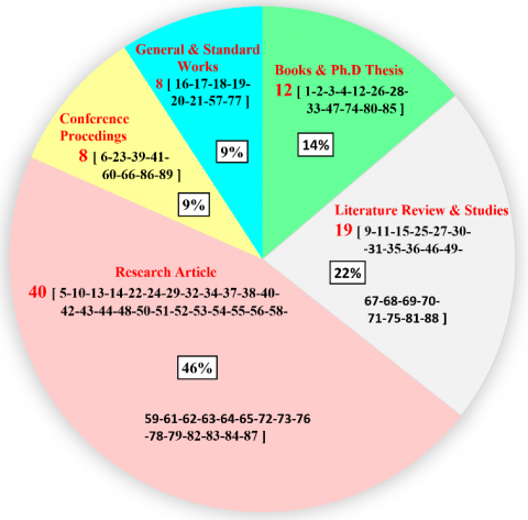
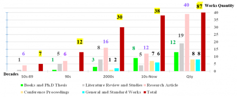
First, a total of 127 references spanning 47 years were gathered for this review. In these existing scientific contributions, two groups are identified in Figure 2. The starting block includes books and Ph.D. thesis, general and standard professional planning works with different norms. On the other side, literature reviews and surveys, specific articles and conference proceedings present diverse mathematical programming and planning models, integrated supply chain.
In the studied discipline, the emphasis is to design, deploy and employ a logistics system that responds most efficiently, to the demands of each end-customer in deterministic and uncertain environments. This type pertains to the category of IPDP Optimization Problems with Pick-up/Delivery that pushes us to extend thinking to new trends for finding how to satisfy customers’ requirements by optimally using necessary resources despite time, capacities, reliability, compatibility and safety constraints. This section presents a literature review of relevant subjects of the ongoing study. It is structured around three aspects: Supply Chain network, characteristics, Integration Modeling and Optimization methods.
Figure 2. Distribution of literature works per type
2.2 State of art of crisis relief supply chains
Crisis Relief military and humanitarian Supply Chain encompasses the determination of requirements, the building up of inventories and capabilities, and the support of transportation and equipment. So, the general problem of optimization is to design a logistics system that responds efficiently to the needs of each customer, like during military and humanitarian operations in a given theater.
2.2.1 Network, processes and decision levels
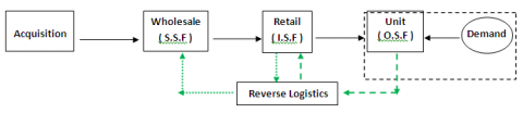
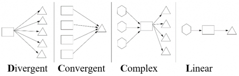
To guide our project, a multistage logistics sustainment model is proposed in Figure 3 as a conceptual approach of the complex military sustainment supply chain structure. It includes demand, retail, wholesale and acquisition stages, along with the reverse logistics stage, as the recycling pipeline for intermediate or service repair level as a “value recovery” effort [9]. Many types of network configurations have been developed in recent works. From a physical flow perspective, SC structures presented in Figure 4 can be classified as divergent, convergent, complex network (combining divergent and convergent structures), or linear. Complex combined network structure integrates forward divergent flows until customers and reverse convergent flows from customers until suppliers [10].
Kress [2] showed that most supply chain networks are organized like military logistics networks, within a complete k-array tree, rooted in the origin, following the three decision levels in Figure 5.
1) Long-term Strategic decisions: national resources and capabilities, locations;
2) Mid-term Tactical decisions: theater-level deployment and employment, planning of best trade-off between load/capacity;
3) Short-term Operational decisions: combat units’ logistics, piloting of flows and scheduling.
Figure 3. Conceptual approach: multistage logistics model
Figure 4. Different structures of supply chain networks
Figure 5. Military logistics decision levels [3]
2.2.2 Crisis response supply chain topology and characteristics
Before-crisis Supply Chain is like a Commercial SC seeking efficiency, cost minimization and best business practices. But during Crisis response time other factors come into play. In fact, a recent analysis of 24 articles in 2024 dedicated to anti-COVID19 management results has shown that the integration of commercial and disaster relief supply chains has become a necessity [11].
For a better comprehension of the characteristics and challenges of military and humanitarian supply chains, a comparison to business supply chains is presented explicitly in Table 1 [2, 12]. The goal of a CRSC is to sustain operations through the best trade-off between demand and supply functions, following cyclic sequences of processes and events [2] at the tactical and operational levels. On demand side, operational centers communicate their needs to tactical or strategic logistic sources. On supply side, materials move via the network that connects the source or intermediate nodes to tactical units. To be more precise, in addition to storage and distribution of commodities, the service of production maintenance is integrated in the optimization problem.
Table 1. Commercial versus crisis relief supply chains
|
Criterion |
Commercial SC |
Crisis Relief SC |
|
Purpose |
Economic Profit |
Survival and Social Impact |
|
Supply Chain Range |
From suppliers’ supplier to Customers’ Customer |
From donors and suppliers to beneficiaries |
|
Operation |
Routine, Long-term, S-L, Uninterrupted |
Rare, Short-term, XL-scale, Interrupted |
|
Environment |
Neutral |
Hostile |
|
Uncertainty |
Demand, Cost, Lead time |
+Deployment, Survival |
|
Cost Consideration |
Mostly economical |
Mostly operational |
|
Graph of Logistic Network |
Static |
Dynamic |
|
Flow |
Sparse, (trucks) |
Massive, (convoys) |
|
Modeling Approach |
Microscopic |
Macroscopic |
|
Service Level Measures |
relatively relaxed Pr[di is satisfied] ³ 0.95, i,…,n “On average 95% of customers are satisfied all the time” |
relatively strict Pr[di is satisfied, i=1,…,n]³0.95 “All customers are satisfied at least 95% of the time” |
Demand and supply description. In any crisis relief operation, operational and tactical decisions are made depending on theater and scenario-based factors during wartime. Demand is non-stationary and affected by possible attrition. Deployed combat or humanitarian units consume diverse supplies that vary from fundamental products (food and water) relatively stable and proportional to the number of troops generally constant, to weaponry and ammunition highly scenario-dependent with larger variance. Here, logistics factors manuals prescribe consumptions’ baselines according to combat day of supply and combat intensity coefficient depending on enemy attrition. Hence, logisticians strive to switch from the sole push strategy to balancing push/pull resupply, and from resource-based to results-based management as follows:
(1) Push strategy: delivery/execution is initiated in response to customers’ orders and;
(2) Pull strategy: delivery/execution is initiated in anticipation of customers’ orders.
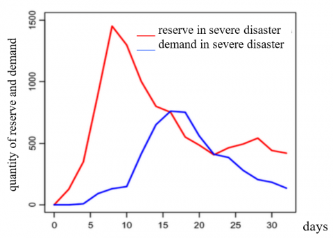
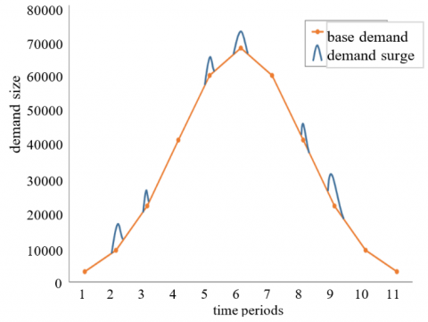
Besides a moderately steady base demand forecast by historical data, demand variability and unpredictability with sudden surges remain climax characteristics of humanitarian and military supply chains, posing significant challenges to forecasting the exact nature and scale of demand. Figure 6 displays different emergency demand patterns that can follow either sometimes a base demand with a bell shape or a more frequent severity-based demand surge [13-15]. The main quantitative examples of these complexity factors are:
(1) Sudden surge in demand for the vital supplies of medical products, food and shelters imposing safety stocks like in (a);
(2) Bottled water can spike from 10,000 units to 90,000 (800% exponential increase) in a few hours after an unexpected earthquake as in (b);
(3) Cultural, Religious and Dietary preferences, as for rice over wheat in some regions;
(4) Supply chain disruptions due to damaged roads or blocked ports that can affect the timely delivery of goods for vulnerable populations by 5 days, especially near epicenter;
(5) In a military context, demand for ammunition, medical kits and fuel might surge depending on combat operations tempo and intensity.
(a) Equilibrium analysis in extreme catastrophe zones
(b) Decomposed demand: Base component and sudden surges
Figure 6. Demand patterns in crisis relief SC [13, 15]
Guiding principles. In crisis relief management, humanitarian supply chain that is a corollary of logistics sustainment of military operations, needs smart supply chains provided that the following principles, mirrored and explained by United States Army Logistics Doctrine [16, 17], are assured. These performance drivers consist of Simplicity, Responsiveness, Flexibility, Attainability, Sustainability, Survivability, Economy (support efficiency), and Integration. Regarding the economy, we distinguish four main categories of costs: inventory holding, maintenance, and transportation, in addition to the disruption costs of shortage and/or backorder penalties. In this context, many national defense organizations issued the “Cost Factors Manual” [18, 19]. These attributes serve as guidelines for critical thinking and careful planning rather than as a checklist. We want to insist here on the modularity aspect of the sustainment nodes. Modularity implies the grouping of inventory, maintenance and transportation functions in one support facility. Hence, a detailed logistics support topology is elaborated in Figure 7 hereafter, to show the Supply Chain Network, modular nodes and flows’ inter-relations.
Figure 7. Theatre logistics support topology: network and flows layout [20]
2.3 Evolution of supply chain optimization
According to the savvy scientist Dantzig, the field of mathematical programming began to grow quickly in the 1950s, when the Rand Corporation released the first commercial software based on linear programming [21].
Numerous theoretical concepts transformed linear programming from an appealing mathematical paradigm into strong large-scale methods and tools that revolutionized the process of practical planning. Hence, appeared successively the Compact Inverse before the Upper Bounds and Secondary Constraints in 1955, then the Decomposition Principle in 1960. Next, Benders discovered the dual form and applied it for the first time in 1962 to solve stochastic programs, and is still widely utilized to solve mixed integer programs. Since 1958, Gomory enriched operations research Integer Programming with the systematic generation of cutting planes, extra necessary conditions, to a current set of inequalities that ensures optimization will result in an integer solution. Its contribution provided another precious approach, different from the earlier work by Dantzig and al on the traveling salesman problem. Gomory theory has been progressively elaborated by many researchers and advanced organizations like IBM, regarding ingenious elimination techniques to resolve 0-1 covering issues. It has been discovered that branch-and-bound is a powerful approach for resolving realistic integer programs. However, the most effective methods up to this point are those that combine branch-and-bound with cutting planes [22, 23].
The majority of useful planning relations were transformed into a system of linear inequalities, and an objective function took the place of the set of guidelines for choosing ideal strategies [24-26]. The development of the simplex method, however, is credited with turning the relatively simple economy linear programming problem into a fundamental approach for the NP-hard systems applied planning. For some samples, the optimal solution can quickly be obtained thanks to a basic simplex or interior method and a basic computer. These contributions remain exceptional because they make it possible to address dynamic scheduling and planning issues over time, especially in the face of uncertainty. The present study is interested in methods for continuous and combinatorial optimization as well as dynamic programming. These tools play an important role in solving planning, scheduling, and inventory control problems, and cover most fields of modern optimization:
(1) We encountered unconstrained non-linear optimization methods that converge to a local optimum or a saddle point, including specific approaches like conjugate-gradient ones. However, many scientists found that meta-heuristics were successful for global optimization regarding evolutionary or genetic algorithms, and the differential evolution method.
(2) From a constrained linear optimization perspective, most reviewed works considered the revised simplex method for linear programming, intended also for linear network optimization or assignment problems.
(3) On another register, authors keen on constrained non-linear optimization have used the standard theorems of the alternative as necessary conditions for mathematical programming, and sufficient conditions for convex functions. They highlighted the usefulness of Lagrangian multiplier and penalty methods for efficient algorithms.
(4) The analysis of reviewed works shows that combinatorial and mixed-integer optimization along with dynamic programming remain by far the most used and preferred methods by supply chain specialists. It has revolutionized operations research, especially in logistics applied mathematics through the dissemination of Branch-and-Bound techniques and their variants including Branch-and-Price, Branch-and-Cut-and-Price. They provide promising results and impactful solutions for decision-makers. Some complex NP-hard combinatorial optimization problems have also become tractable thanks to successful meta-heuristics among which Tabu search and more recent nested partitions methods are very promising techniques.
However, due to the challenging real-world volatility of the 1990s, stochastic programming, despite its difficulty, has become an exciting field of research and applied science that has solved some important long-term planning problems in many countries. Hence, great optimization methods have emerged to solve dynamic multi-sector programs, through combining the Nested Decomposition Principle based on staircase structure, the ranking selection and the use of matching processors. Since then, the application of these methods has proven huge results in the building of economic growth strategies [24, 26]. The breakthrough advancement is the capacity to specify broad goals and figure out the optimal solution for complex practical decision-making problems.
For a good understanding of global supply chain optimization and uncertainty mitigation, the author gives in Table 2, an interesting outline of different modeling methods each with specific type and characteristics, highlighting the conceptual, simulation and mathematical model. In this last one, each decision-maker or researcher must initially define the problem characteristics, network topology (nodes and flows), relevant decision variables to optimize, problem constraints, and the nature of the data set. These inputs help them classify optimization problems and adopt the most suitable Objective Function and Constraints’ formulation, mathematical modeling, and powerful solution method. When discussing the logic of optimization models, many academics notice that while constrained programming (CP) permits coming up with possible outputs, linear programming (LP) and Integer Linear Programming (ILP) help reach optimal solutions. However, many authors believe that these programming approaches have specific limitations when it comes to solving large-scale problems with wide solution spaces and accurately representing some of the stochastic and dynamic aspects of optimization problems.
Table 2. Methods of supply chain modeling
|
Modeling Characteristics |
Modeling Types |
||
|
Conceptual Model |
Mathematical Model |
Simulation Model |
|
|
Represent chain as: |
Diagrams and Descriptions |
Functions and Equations |
Objects et Interactions |
|
Solutions found through: |
Verbal Reasoning |
Optimizer and Solvers (IBM/CPLEX-LINDO) |
Experiments (Monte Carlo) |
|
Best application for: |
Understanding Share |
Optimal Performance |
Realistic Forecasting (like Demand) |
Explicitly, records are identified from databases and registers and then screened. After a thorough selection, Retrieved and eligible reports give the studies and respective scientific contents to include in the review and determine gaps’ findings. In general, the reviewed literature is structured according to four main specifications, depending on Problem definition; Objective function; Mathematical modeling; Solution methods (LP, MILP, MINLP, Stochastic Mixed Integer Programming (SMIP), and Mixed Integer Goal Programming (MIGP)); and Results (outputs/variables): transportation amount, vehicles and demand satisfaction, inventory, location/allocation, and production quantity. In our case, we’ll focus on integrated IPDP with Pick-up/Delivery.
Table 3 and Figure 8 detail the historical evolution of literature works investigated during our study. Getting informed of past and recent studies by well-known specialized scientists and professionals, the obtained results of this literature review and gaps findings demonstrate the originality of the contribution of the proposed work to the scientific research community.
Table 3. Reviewed works per periods from 1954-2024
|
Publication Type |
50s-89 |
90s |
2000s |
10s-Now |
Qty |
|
Books and Ph.D Thesis |
|
1 [1] |
3 [2-28-47] |
8 [3-4-12-26-33-74-80-85] |
12 |
|
Literature Review and Studies |
1 [25] |
5 [9-36-67-70-88] |
8 [31-35-49-68-69-71-75-81] |
5 [11-15-27-30-46] |
19 |
|
Research Article |
6 [5-22-76-79-83-84] |
6 [42-43-53-59-61-62] |
16 [10-24-32-44-50-51-52-54-55-63-64-65-72-78-82] |
12 [13-14-29-34-37-38-40-48-56-58-73-87] |
40 |
|
Conference Proceedings |
|
|
1 [60] |
7 [6-23-39-41-66-86-89] |
8 |
|
General and Standard Works |
|
|
2 [16-18] |
6 [17-19-20-21-57-77] |
8 |
|
Total |
7 |
12 |
30 |
38 |
87 |
Figure 8. Historical evolution of reviewed literature
3.1 Integration: Climax of supply chain revolution
The integration of supply chain echelons and functions is a major turning point in decoupling organizations’ outputs and benefits within modern economies and industries. When optimizing a situation for one issue but neglecting the other, some of the costs of the disregarded issue or function might be very high. Decisions that significantly affect one another must be coordinated to guarantee the supply chain operates efficiently and agile [27]. Shapiro, among other well-known authors, contributes widely in elevating the value of logistics science in strategic planning and management from an unbiased perspective [28].
In our supply chain model, decisions aim at improving the analysis approach of sustainment supply chains from a sequential functional dimension to more integrated and global management perspective that is still at the beginning stages in scientific literature, especially in military, humanitarian and other crisis management operations. We investigate four types of Supply Chain Integration:
(1) Space-time or Geographical Integration;
(2) Functional Integration;
(3) Inter-organizations Integration: From a domain-based to Inter-domains structure or Vertical Integration [29];
(4) Decisional Integration combining strategic, tactical and operational decisions in one inclusive model.
3.1.1 Space-time integration
It refers to a dynamic geographical integration from local to multi-echelon or worldwide supply chain network and flows, where multi-period planning means finding the optimal solution for the model in a finite or infinite planning horizon, in place of a single period one. Given the scale and complexity of such optimization problems, the interesting reviews of Bhatnagar, Chen and al. address the issues of supply chain coordination and integration under two types [9, 10]. The first concerns alignment within the same function at several stages of the supply chain, a Multi-Plant Coordination Problem.
3.1.2 Functional integration
This transition from one function-dominated to a flow-dominated supply chain, promoting coordination between functions in one or more echelons, is the second type proposed by the same authors, as a General Coordination Problem [9, 10]. The integration of Inventory, Production and Distribution decisions in one global optimization problem like in our study is a relevant illustration of this more inclusive integrated model. Table 4 illustrates most dedicated integrated supply chain optimization models, studied in literature. Scientists started with network design or one function pure optimization problem, and have progressively investigated Inventory-Distribution, Inventory-Production or Production-Distribution planning. Others investigated sustainable resilient supply chain in emerging economies [6]. However, only a few works discussed Integrated Inventory-Production-Distribution planning decisions concentrating on the tactical and operational levels, and/or incorporating potential integration with strategic location decisions.
Reviewed works imply that there are two main reasons why integrated optimization of these large-scale supply chain problems is challenging. Throughout the supply chain, various facilities and/or choices may have opposing objectives. A lot of studies show that sequential analysis yields only to locally optimal decisions that could play as a structural constraint to the global supply chain. But, modern successful organizations appeal for global optimization that allows service level satisfaction while minimizing total sustainment cost through integrating and aligning simultaneously inventory, production and distribution processes and decisions with aggregate demand [30]. This is the reason behind the study of research works focusing on modeling and resolution of integrated Inventory Production Distribution problems (IPDP).
Table 4. Main integrated supply chain planning models
|
Integrated Models |
Inventory |
Production |
Location |
Distribution |
|
|
DS |
Rout |
||||
|
Lot Sizing (LSP) |
X |
X |
|
|
|
|
Inventory Distribution (IDP) |
X |
|
|
X |
|
|
Inventory Routing (IRP) |
X |
|
|
|
X |
|
Location Distribution (LDP) |
|
|
X |
X |
|
|
Location Routing (LRP) |
|
|
X |
|
X |
|
Inventory location (ILP) |
X |
|
X |
|
|
|
Inventory Production Routing (IPRP) |
X |
X |
|
|
X |
|
Inventory Production Distribution (IPDP) |
X |
X |
|
X |
|
3.2 Closed-loop supply chain optimization
The research project surveys particular planning problems for supply chain optimization including forward, reverse, decoupled, integrated, or coupled types. This section's goals are to organize the relevant literature review and categorize optimization models, upon four general characteristics e.g. problem description, supply chain structure, goals or outputs, and solution methods. This taxonomy paves the way and motivates our detailed description and contribution to an inclusive integration inventory-production-distribution decision model. Depending on planning and scheduling objectives, optimization aims at finding the best order of tasks’ fulfillment and resource allocation to maximize outputs or minimize total cost during the shortest time. This approach fits more likely for production processes as presented by Hillier and Lieberman [31]. The majority of literature works consider sequential or decoupled optimization regarding inventory, production, distribution and MILP facilities location models, evaluating from one period, single commodity, simple uncapacitated facility location model to more elaborated models.
However, Jayaram et al. [32] and Fleischmann et al. [33] have surveyed specific integrated forward/reverse supply chain problems that include capacitated multi-period, multi-stage and multi-commodity models through either MILP or MINLP. Hence, to solve integrated supply chain problems, optimization models and algorithms moved progressively from single-function pure inventory problems, production, distribution, network design [34] or vehicle routing problems [35], to more integrated approaches, such as location-routing [36], location-allocation [37, 38], inventory routing, production routing or inventory production distribution (IPDP) problems that prove to be more complicated as in [39, 40].
3.2.1 Pure inventory optimization model
The optimization of pure inventory problems, or the role of inventory management, serves to identify the best mix of anticipation, cycle, safety, pipeline or/and decoupling stocks. In 2014, Graves Stephen [24] and Chen [41] investigated successively many types of deterministic and stochastic-demand inventory models: economic order quantity (EOQ); single-period-like newsvendor model; and multi-period with periodic review, base stock policy and continuous review, (R,Q) policy.
If not, stock-outs result in lost sales very quickly. Table 5 summarizes the main inventory models depending on the following characteristics:
(1) Demand. Constant, deterministic, stochastic.
(2) Frequency. Single period, multi-period, finite, infinite.
(3) Commodities. Mono or multi-commodity.
(4) Capacity. Limited or uncapacitated order/inventory limits.
(5) Service. Satisfy all demand, allowed shortages, or meet all demand points but with a certain level.
Being the cornerstone of inventory management, stocking control helps ensure at the lowest possible cost, that the proper quantity of stock is available for sustaining the organization's targeted fill rate in the market. In order to ensure that customers are served within lead time throughout the supply chain, decision-makers must establish and oversee specific service levels and logistics strategies.
Table 5. Classification of inventory models [24]
|
Model |
EOQ |
Newsvendor |
Bas Stock |
(R, Q) |
|
Horizon |
Infinite |
Single |
Infinite (Periodic Review) |
Infinite (Continuous Review) |
|
Demand |
Constant |
Stochastic |
Stochastic |
Stochastic |
|
Lead time |
0 |
0 |
L>0 |
L>0 |
|
Decision variable |
Order quantity Q (Order period T) |
Order quantity Q |
Review period T •Order-up-to level S |
Reorder point R Order quantity Q |
|
Optimal Solution |
$\begin{array}{r}\mathrm{Q}=\sqrt{\frac{2 K \mu}{\mathrm{h}}} \\ \mathrm{T}=\frac{\mathrm{Q}}{\mu}=\sqrt{\frac{2 K}{\mathrm{~h} \mu}}\end{array}$ |
$P(D \leq Q)=\frac{C_u}{C_\mu+C_o}$ |
$\begin{gathered}\mathrm{T}=\sqrt{\frac{2 \mathrm{~K}}{\mathrm{~h} \mu}} \\ \mathrm{S}=\mu \mathrm{T}+\mathrm{L}+\mathrm{z \sigma} \mathrm{T}+\mathrm{L}\end{gathered}$ |
$\begin{gathered}\mathrm{R}=2 \sigma \mathrm{T}+\mathrm{L} \\ \mathrm{Q}=\sqrt{\frac{2 \mathrm{k} \mu}{\mathrm{h}}}\end{gathered}$ |
The evaluation of results has shown that decoupled approaches are rapidly deceiving when inventory, production and distribution costs belong to the same scale. So, these functions must be considered simultaneously within the same model.
3.2.2 Multi-functional optimization
If one pure inventory optimization problem is difficult to solve, it is evident that large-scale integrated closed-loop multi-echelon multi-function planning models, such as Inventory Routing, Production Routing, or Inventory Production Distribution (IPDP) problems, probe to be more complicated. We are interested in integrated optimization approaches that consider simultaneously two or more functions to minimize the total cost of the dynamic global supply chain.
Table 6 summarizes reviewed works regarding respectively single and multi-echelon supply chain optimization. No need to mention that multi-echelon Inventory Production Distribution Problems probe to be more complex to resolve as they imply many more variables and constraints to deal with.
Table 6. Reviewed works regarding single-echelon and multi-echelon integrated supply chain optimization
|
References |
Number of |
Capacity Limitation |
Demand |
Characteristics & Decision Variables |
Solution Methods |
||||||
|
Periods S/M |
Commodities S/M |
Plants S/M |
Inventory |
Production |
Det/Sto |
Inventory P/DC/C |
Production |
Loc |
Distribution DS/Rout |
||
|
Single Echelon Supply Chain Models |
|||||||||||
|
Archetti et al. [26] |
M |
S |
S |
X |
|
Det |
P; C |
X min |
|
Rout |
Branch-and-Cut |
|
Chandra and Fisher [42] |
M |
M |
S |
|
|
Det |
P; C |
X |
|
Rout |
Local Improvement Heuristic |
|
Fumero and Vercellis [43] |
M |
M |
S |
|
X |
Det |
P; C |
X |
|
Rout |
Lagrangian Relaxation |
|
Archetti et al. [44] |
M |
S |
S |
X |
|
Det |
DC; C |
|
|
Rout |
Branch-and-Cut |
|
Solyali and Sural [45] |
M |
S |
S |
X |
|
Det |
P; DC |
|
|
Rout |
Branch-and-cut and Tour-Based Heuristic |
|
Adulyasak et al. [46] |
M |
S |
S |
X |
X |
Sto |
P; C |
X |
|
Rout |
Branch-and-Cut and Benders Decomposition |
|
Nananukul [47] |
M |
S |
S |
X |
X |
Det |
P; C |
X |
|
Rout |
Reactive Tabu Search and Path Relinking |
|
Ruokokoski et al. [48] |
M |
S |
S |
|
|
Det |
P; C |
X |
|
Rout |
Branch-and-Cut |
|
Lei et al. [49] |
M |
|
M |
X |
X |
Det |
P; DC |
Min |
|
DS then Rout |
Decomposition Approach |
|
Bard and Nananukul [50] |
M |
S |
S |
X |
X |
Det |
P; C |
X |
|
Rout |
Reactive Tabu Search |
|
Bard and Nananukul [51] |
M |
S |
S |
X |
X |
Det |
P; C |
X |
|
Rout |
Branch-and-Price |
|
Solyali and Süral [52] |
M |
S |
S |
X |
|
Det |
DC; C |
Min |
|
Rout |
Lagrangian Relaxation |
|
Multi-Echelon Supply Chain Models |
|||||||||||
|
Pirkul and Jayaraman [53] |
S |
M |
M |
X |
X |
Det |
P; DC |
|
X |
DS |
Lagrangian Relaxation |
|
Jayaraman [54] |
S |
M |
M |
|
X |
Det |
P; DC |
X |
|
DS |
Analytical Approach With Aggregate Production Planning |
|
Jayaraman and Pirkul [55] |
S |
M |
M |
|
X |
Det |
-- |
X |
X |
DS |
Lagrangian Relaxation |
|
Crisis Relief Supply Chain Optimization |
|||||||||||
|
Zhu et al. [13] |
M |
M |
M |
X |
X |
Sto |
DC |
|
|
DS |
Ranking and Multi-objective Fuzzy Optimization |
|
Song et al. [14] |
M |
M |
M |
X |
|
Sto |
P; DC |
X |
|
DS |
(s, S) Policy replenishment, LP Relaxation with Demand base and surge |
|
Noyan et al. [56] |
M |
M |
|
|
|
Sto |
DC |
|
X |
DS/Rout |
branch-and-cut and Benders Decomposition |
|
Minic et al. [57] |
M |
M |
|
X |
|
Det/Sto |
DC; C |
|
X |
DS/Rout |
Extensive Stochastic method using scenarios-demand Sampling |
|
Doyen et al., 2011 [58] |
M |
M |
|
X |
|
Sto |
DC; C |
|
X |
DS |
Heuristic-based Lagrangian Relaxation |
Chandra and Fisher [42] figure among the prior investigations valuing the integration of production and distribution decisions in comparison with decoupled optimization of production planning and transportation problems. The findings of computational analysis highlighted that the coupled model offers potential cost savings of 5 to 20%. Fumero and Vercellis [43] also developed a synchronized production-inventory-distribution schedule where they used Lagrangian relaxation to solve the integrated MILP problem. In 1996, Pirkul and Jayaraman [53] modeled a cost minimization problem to simulate an integrated multi-commodity, tri-echelon, plant capacity, and warehouse location system. They employed a heuristic approach to solve the issue and Lagrangian relaxation (LR) to determine the lower bound. After three years, Özdamar and Yazgac [59] resolved an integrated production-inventory-routing problem through a hierarchical method. Following collective aggregated decision-making, they improved the planning model to a daily schedule.
From then, many scientists proposed some integrated optimization models for production and distribution planning, to coordinate optimally relevant interrelated supply chain decisions, like capacity management, inventory allocation, and vehicle routing. Forma et al. [60] defined and formulated an integrated SCM problem, including procurement, inventory, production and transportation decisions. It is now used as a foundation for contrasting different functional decomposition techniques. Additionally, it has modeled the potential savings from combining tours linked to the transportation of finished goods and raw materials together, as well as the potential to use both owned and third-party transporters. This strategy proved to be more economic and environmental. Qu et al. [61] developed a decomposition method for an integrated inventory-transportation model with stochastic demand for multi-commodity. They adopted isolated computation for inventory and routing decisions before synchronizing them suitably.
However, many researchers like Federgruen and Tzur [62] introduced effective time-partitioning heuristics to solve multi-commodity production/distribution Supply Chain problems, and decomposed the planning horizon into smaller ones, with possible extension to geographic application. They applied it to a multi-location dynamic lot-sizing problem, elaborating then a heuristic for the one warehouse multi-retailer model of a two-echelon distribution network delivering distinct items. Computational results have shown that the partitioning heuristics were efficient, leading to a close-to-optimal solution within 1.5% of optimality, even with up to 150 periods of planning horizon and large numbers of retailers and commodities. An interesting optimization model was developed by Berman and Wang [63] to integrate simultaneously inventory and distribution functions with decisions regarding the supply chain network and location of cross-docking sites. Lately, Toptal and Çetinkaya [64] aligned the supply chain demonstrating through analytical and numerical results, interesting cost enhancement. But, they discovered that this performance comes from the variation in cost criteria. In the framework of integrated supply chain optimization, alignment of inventory and distribution system was conducted in 2007 by Archetti et al [44]. They performed a branch and cut algorithm for a MILP and compared the results of two relaxations of the problem. Lei et al. [65] proposed a smart effective two-phase approach to solve an integrated production-inventory-distribution routing problem through cost minimization while satisfying customers’ demand. After solving the original problem when routing costs were estimated only by direct shipment costs, they resolved the integrated supply chain problem through the consolidation of the inventory, production and direct shipment decisions, already obtained in the first phase with routing costs and constraints.
An in-depth study is given in part V dedicated to discussing potential solution methods. From then, reverse logistics captivated substantial consideration from researchers who published many literature reviews, surveys and models. Amin and Zhang [66] proposed in 2012, a closed-loop supply chain network configuration based on return-recovery recycling through a MILP model. The model aimed at maximizing profit from the optimal quantity of remanufactured products resent to the secondary market. Fleishman et al. [67] reviewed and categorized quantitative mathematical models for reverse logistics distinguishing three key functions optimization: distribution planning, inventory and production planning. Jamsa [68] and Rubio et al. [69] provided a literature review of interesting works and issues, along with case studies and opportunities of research, regarding reverse logistics planning and network design published since the 1990’s.
3.2.3 Forward/reverse supply chain optimization
It is only during the three last decades that many integrated optimization models were meticulously investigated and developed either for reverse or closed-loop supply chain planning and/or network design as illustrated in the practical case presented by Chekoubi et al [39]. Jayaraman [54, 70]. were among the top contributors in this field. In 1999, they provided a MILP decision model for the design of reverse logistics networks with a pull system determined by customers’ demand for returned and repaired products [32, 71]. Fleischmann et al. [33] showed that an integrated approach optimizes simultaneously the forward and reverse flows providing considerable cost savings. In the wake of this work, Salema et al. [72] expanded Fleischmann’s model to multi-product network design under demand uncertainty paving the way for very promising outcomes.
3.3 Crisis relief supply chain optimization
Some key papers proposed valuable inventory, location, production and distribution models applying useful mathematical optimization techniques and algorithms. To boot, the premier practical reference book [12] expands the academic understanding of crisis response supply chain through sharing applications lessons learned by professionals in daily logistics and worst case scenarios during recent natural and manmade disasters alleviation operations. In 2022, Zhu et al. validated a collaborative fuzzy-based optimization method that ensures both integrative emergency suppliers’ evaluation and a sufficient reserve material safety inventory to avoid stockouts and minimize human and material damages, through uncertainty mitigation by a fuzzy interval control ante-, during and post-phases [13]. Habib et al. also offered an exhaustive systematic review of most relevant scientific contributions in the two last decades [15].
If deterministic models are more utilized, some authors like Salmeron and Apte elaborated a two-level stochastic location-distribution-inventory optimization model but used the exact solution method, branch-and-bound algorithm, for scenario-dependent equipment and budget allocation prepositioning before a natural crisis starts so that to satisfy variable demand and minimize the expected number of casualties [73]. Noyan et al. [56] and Ozdamar [74] developed disaster relief preparedness and response models addressing successively strategic mitigation decisions of warehouse and inventory prepositions to reduce response time and both tactical fleet size decisions and operational last-mile distribution decisions and casualties’ evacuation. Throughout Scenario-based 2-stages Stochastic Programming models, the author maximized the anticipated accessibility score using an adapted branch-and-cut decomposition algorithm, applied successively in the recent Turkey earthquake.
However, the advanced contributions in the studies [57, 58] greatly inspired us on the design and formulation of our integrated optimization model. They elaborated multi-echelon disaster relief supply chain optimization models and algorithms, through progressive 2-stage deterministic-to-stochastic programming approach. The total cost minimization of facility location, inventory holding, distribution and shortages subject to some realistic constraints was expressed as a MILPdeterministic equivalent model, tackled by a heuristic approach based on Lagrangian Relaxation and by vehicle symmetry breaking constraints that value the impact of branch-and-bound technique.
Most recently, Guide Jr. and Van Wassenhove [75] gave an exhaustive summary of the development of closed-loop supply chain design and planning research throughout the following five successive stages: From remanufacturing as a technical problem to estimating the reverse logistics steps, before aligning the reverse supply chain, and closing the loop. After a thorough selection, 88 retrieved and eligible reports give the studies and respective scientific contents to include in the review and determine gaps’ findings.
3.4 Research gap findings
So as outlined, the great part of the reviewed literature on supply chain optimization planning models has targeted forward and reverse logistics separately and hasn’t fully considered the integrated closed-loop configuration. However, few studies have investigated the integrated forward/reverse logistics functions problems of multi-echelon multi-commodity CRSC optimization in a multiple time horizon. Our review investigated some of the most important methods and tools, previously used for situation-based modeling and solving supply chain management problems. So, it inspires us to describe, simplify then formulate a real-world problem for possible analysis, before designing efficient algorithms to obtain high-quality solutions for impactful decision-making.
Further significantly to our knowledge, none of the previous research works has tried to find efficient strategies for a multi-period multi-echelon multi-commodity closed-loop supply chain with non-stationary demand through an integrated Inventory-Production-Distribution planning model with pick-up/delivery. Based on Table 6, the proposed model presents the characteristics detailed in Table 7.
To motivate our future contribution and model development, this literature review inspired us to situate the proposed integrated model among three classical optimization sub-problems: Multi-Bin Packing Problem (MBPP) as in the work [76], Inventory Distribution Problem and Resource-Constrained Production Scheduling Problem (RCSP).
Table 7. Research gap: Defining our problem
|
Discussed Problem |
Single/Multi |
Capacity Limitation |
Fwd/Rev/ Closed-Loop |
Demand |
Inventory |
Production/ Maintenance |
Distribution |
|||
|
Echelon |
Period |
Commodity |
Prod. |
Distrib. |
Det/Sto |
P/DC/C |
DS/Rout |
|||
|
CIPDND |
M |
M |
M |
X |
X |
Closed-loop |
Det and Non-stationary |
P; DC |
X |
DS |
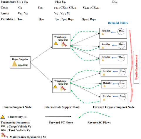
Figure 9. Multi-period supply chain network
In that Multi-Stage Multi-Period IPD Problem as described in Figure 9, the presence of non-stationary demand, forward and reverse flows and hostility attrition, along with commodity clustering and commodity-vehicle compatibility constraints, make this optimization model unique and valuable for military and humanitarian logistics planners, as well as electronic and vehicles industries. It seeks to enhance both supply chain efficiency and safety with utmost customers’ satisfaction. As far as we know, this problem is the first to address diverse new real-world features of military and humanitarian supply chains has not been dealt with before in literature works.
Hence, Figure 9 shows a simplified schematic representation of the multi-period model’s structure:
(1) 1 Source of Support Node with consolidation, 2 Intermediate Support Nodes with consolidation and 6 Forward Organizational Support Node with End-User Demand, considered Customer Demand Node.
(2) Both Warehouses are modular nodes with two or more functions integration.
This study considers an integrated logistics sustainment model that coordinates the in-theater core functions of Supply, Maintenance and Transportation upstream and downstream, taking into consideration most of relevant parameters and constraints linked to the required sustainment performance level of fighting units. So, we will try to answer this question: Given a dynamic three-echelon multi-period military supply chain network,
4.1 Problem description
A three-echelon multi-period logistics sustainment network model is adopted where each node is composed of inventory, maintenance and transportation facilities. This tactical supply chain falls within the category, of Inventory-Production-Distribution on nodes for it aims at satisfying the requirements of a set of customers that can be represented by nodes on a network. It is a dynamic multi-stage multi-period IPDP Problem as detailed in Figures 7 and 9. The situation we look at is a single Source of Supply that delivers logistic support to warehouses, then retailers through the Military/Humanitarian Logistics Sustainment Network. We consider four types of flows: transportation trucks and helicopters, new commodities, and returned commodities repaired by the maintenance workforce. We also consider delivery disruption with backorders (or shortages) cost penalties. The concerned closed-loop divergent supply chain network is an integrated three-echelon network with both forward and reverse flows through one Theater Source Support Node (SSF), two Intermediate Modular Support Nodes (ISF) and three Forward Organic Support Nodes (FOSF) for each ISN. Due to safety concerns, lateral supply between both the ISFs (Warehouses) and the FOSF (Retailers) is not allowed. An ISF is to be assigned at least one Retailer, but each Retailer must be assigned exactly one ISF.
4.1.1 Coding of the problem: Model’s features
Capacitated Flows. Flows in the logistics network comprise two types. Commodities: new commodities such as: ammunition, food, water, spares and POL and recycled commodities referring to repaired returned commodities. And Transportation vehicles that carry the supplies: Trucks and Helicopters of heterogeneous classes and two modes.
Distribution. A weight per pallet (W) is associated to each pallet and a payload (PC) and bulk (BC) capacity is associated with transportation assets. Arrows of the bottom of figure show some potential transportation relationships between commodities on one hand and between commodities and means of transportation on the other. For instance, some products are never transported together because of technical and tactical danger (e.g mixing ammunition and oxygen bottle in one 5 Tons Expansible Van Truck).
Production. A service labor capacity is associated with battlefield commodity failure, implying maintenance workforce skill at each location. Maintenance service encompasses three-level maintenance system comprising organic maintenance level, intermediate maintenance level and theater level operations. This multi-level system provides timely repairs and necessary evacuations, ensuing in rapid servicing of equipment and returned products, and quick return of items to customers’ units in an operational status, as these organizations are developing new multifunctional maintenance facilities to meet 21st century requirements [77].
Limited resources. They include only most critical and restricted resources in the planning model. They consist of vehicles and technicians’ workforce that refer respectively to transportation and production.
Demand. Deterministic, non-stationary (advancing) but must be periodically revised according to environment-technical and tactical attrition. It consists of multi-commodity: finished and returned repaired ones.
Balancing Push and Pull Resupply. The dual behavior of demand motivates us to reflect on moving progressively from push strategy to the best trade-off between push and pull resupply for customers’ requirements satisfaction. At the forward flow, commodities with valid usage rates require pushed automatic resupply, suitable for getting stocks of common-user items. It is better to use pull strategy requisitions for variable usage rate needs of commodities, drawn through a divergent network. In reverse logistics, flows of defective returned products are picked up and shipped following push principles through a semi-convergent network. A proportional quantity of demand from each customer node in each period satisfied is reversed items with a known disposal fraction.
Contemporary logistic inventiveness seeks to reduce costs, develop pull resupply for maximum efficiency, and grow speed, forecasting and visibility of resupply, even for products like returned parts and main items [16, 17].
Multi-period Planning Horizon. A CRSC is normally stratified into time-periods (days, hours) needing different levels of supply as shown in Figure 8. The time-dependent dynamics of sustainment flows are considered in our proposed model with the use of two modes of transportation means: trucks and helicopters of heterogeneous classes. The schedule or sequences of production and distribution runs are assigned to any period.
Facility Capacity. Capacitated facilities except for the Source Support Node which can supply all requirements. Only most critical or limiting resources in the optimization problem will be considered like transportation resources (vehicles), production resources (workforce), limited inventory capacity and safety stock, be it known that facilities to be opened are determined.
Relevant Costs. Inventory holding costs, variable production cost, variable delivery vehicle cost, and imperfect customer service penalty cost: when demand is back-ordered or isn’t filled on time. There is a linear relationship between production quantity and resource usage.
And road freight cost is estimated as a function of distance and load. The Cost per driving hour is defined as the hourly cost of operating ground mobility or transportation vehicle that covers fuel costs, consumables like washers and bearings, and the repair of major systems and subsystems, such as engines at Intermediate-level repairable. So, the variable transportation cost is calculated with its hourly cost rate, cruising speed and traveled distance or time. In short, we distinguish three main categories of logistics costs:
(1) Inventory holding costs and Disruption costs: shortage or backorders penalty;
(2) Maintenance costs: Hourly cost rate ($/h) x Labor hours;
(3) Transportation costs.
Planning Decisions to include in the model. allocation quantities, distribution decisions in terms of fleet size (number of vehicles), transportation and demand satisfaction quantities, location decisions for the two Intermediate Support Nodes, production quantities and schedule for the repair of returned commodities, inventory holding quantities
Modelling Approach with MILP Programming, supporting both forward supply, recovery and resupply tasks, adapted to military/humanitarian operations’ sustainment and different kinds of industries like in vehicle and electronic industries surveyed by Üster et al. [78].
4.1.2 Assumptions: Simplified supply chain problem
To limit the complexity of our optimization model, the present study integrated the most impacting functions of inventory, production and distribution in terms of efficiency and customers’ satisfaction, which is supposed to be a large-scale problem. From then on, the following assumptions are considered:
Then, we will try to find feasible support plans that improve the efficiency, responsiveness and robustness of the model.
4.2 Problem formulation
The optimization problem is to determine the most efficient Closed-Loop Inventory-Production-Distribution Plan to meet Non-stationary Demand (CIPDPND) within a global supply chain. It is a MILPproblem that minimizes the total cost of an integrated forward/reverse supply chain while satisfying customers’ demands. We provide an optimization model where we define the objective function, decision variables, and constraints through a MILP formulation. Nomenclature defines the used Sets, Indices and Parameters.
4.2.1 Decisions variable
|
Iskt, Ijkt |
Inventory holding quantity of commodity k at support facility f at end of period t; |
|
Fsjkt |
Quantity of commodity k shipped from SSF s to ISF j by the eth vehicle of class v of SSF node s in period t, for e=1,…, Lvs, v∈Vs, s∈S, k∈Kv, t∈T. |
|
Fjnk |
Quantity of commodity k shipped from ISF j to customer n by eth vehicle of class v of SSF node j in period t, for e=1,.,Lvj, v∈Vj, j∈J, k∈Kv, t∈T. |
|
Pjnkt |
Production workforce for maintenance of commodity k at support facility f during time-period t; |
|
Bjnkt |
Amount of shortages(unsatisfied demand) of commodity k at Intermediate support facility j from demand point n in period t; |
|
Ysjkvt |
Number of transportation vehicles of class v necessary for shipment of commodities k from source s to intermediate support units j in period t; |
|
Yjnkvt |
Number of transportation vehicles of class v necessary for shipment of commodities k from intermediate support unit j to demand locations n in period t; |
|
Xsjkevt |
=1 if eth vehicle of class v of SSF s is used to ship commodity of class k to ISF j in period t for e=1,…, Lvs, v∈Vs, j∈J, k∈Kv, t∈T; 0 otherwise. |
|
Xjnkevt |
=1 if eth vehicle of class v of ISF j is used to ship commodity of class k to customer n in period t for e =1,., Lvj, v∈Vj, j∈J, n∈N, k∈Kv, t∈T; 0 otherwise. |
|
Yjot |
Number of maintainers o needed for maintenance of commodity k at intermediate support facility j |
4.2.2 Objective function and constraints
Objective function. The objective function minimizes the sum of the inventory holding costs at source and intermediate support facilities, the forward transportation costs from source to intermediate support facilities and from these facilities to the demand locations, and the shortages penalty costs from each demand location to its intermediate support facility, for all commodities; in addition to the reverse recovery costs from each demand location to its intermediate support facility and the production costs at this facility, for the commodity k’, over the planning horizon of T periods. Shortage penalty costs are considered linear in the number of shortages from each demand location in each period. No need to mention that we used a combination of many extensions to the basic IPDP model before arriving at the proposed formulation.
$\overbrace{\operatorname{Min} \sum_{t=1}^T(\sum_{k=1}^K(\mathbf{g}_{\mathrm{sk}} * \mathbf{I}_{\text {skt }}+\sum_{j=1}^J}^{\text {Inventory Holding}} \overbrace{(\mathbf{g}_{\mathrm{jk}} *\mathbf{I}_{\mathrm{jkt}}+\sum_{v=1}^V(\Sigma_{e=1}^{L_{v s}} \mathbf{c}_{\text {sjkt }} *\mathbf{F}_{\text {sjvekt }}+\sum_{n=1}^N (\Sigma_{e=1}^{L_{v j}}(\mathbf{c}_{\mathrm{jnkt}} *}^{+\qquad \text {Forward Distribution}\qquad+\qquad \text{Reverse}}\overbrace{\mathbf{F}_{\text {jnvekt }}+\mathbf{c}_{\mathrm{jnkt}}{ }^* \mathbf{R}_{\text {njvkt }}) }^{\text{Recovery}}\underbrace{+\mathbf{m}_{\mathrm{jk}}{ }^* \mathbf{P}_{\text {jnkt }}}_{+\text {Production }} \underbrace{+\mathbf{q}_{\mathrm{jk}}{ }^* \mathbf{B}_{\text {jnkt }}}_{+\text{Shortage Penalty}})))))$ (1)
Subject to the following constraints:
Demand constraints Eqs. (2)-(4):
$\mathrm{F}_{\text {jnkt }} \geq \alpha^* \mathrm{~d}_{\text {njkt }} \quad \forall \mathrm{k}, \mathrm{n}, \mathrm{j}$ (2)
$\mathrm{B}_{\text {jnkkt }} \leq(1-\alpha) * \mathrm{~d}_{\text {mikt }} \quad \forall \mathrm{k}, \mathrm{n}, \mathrm{j}$ (3)
$0<\beta \leq \alpha \leq 1 \quad \forall \mathrm{k}, \mathrm{n}, \mathrm{j}$ (4)
The demand of each customer must be satisfied more than the desired level. Deterministic demand is aggregated into a set of demand locations towards higher-stage support facilities ISFs. Shortage quantity for each commodity from each demand location has to remain very low so that the determined demand satisfaction level α is assured to be more than the minimum tolerated rate β.
Inventory constraints Eqs. (5)-(8): Inventory balance constraint
$\sum_{j=1}^J\left(I_{j k t}+\sum_{n=1}^N P_{j n k t}\right)+\sum_{v=1}^{V_s} \sum_{e=1}^{L_{v s}} F_{\text {sjvekt }}-\sum_{n=1}^N \sum_{\mathrm{v}=1}^{V_j} \sum_{e=1}^{L_{v j}} F_{j n v e k t}=\sum_{j=1}^J I_{j k((t+1)} \quad \forall k, v, n, j$ (5)
$I_{j k t}+\sum_{n=1}^N P_{j n k t} \geq \sum_{n=1}^N F_{\text {jnkt }} \quad \forall k, n, j$ (6)
$\mathrm{W}_{\mathrm{k}} *\left(\mathrm{I}_{\mathrm{jkt}}+\sum_{\mathrm{n}=1}^{\mathrm{N}} \mathrm{P}_{\mathrm{jnkt}}\right) \leq \mathrm{Ujk} \quad \forall \mathrm{k}, \mathrm{n}, \mathrm{j}$ (7)
$I_{j k t}+F_{\text {sjkt }}+\sum_{n=1}^N P_{j n k k} \geq \sum_{n=1}^N\left(F_{j n l k}+B_{j n k k t}\right) \forall k, n, j$ (8)
Constraint (5) explains dynamic inventory balance quantity between t and t+1.
The supply of a commodity at each facility is either held in inventory or routed to a demand point to satisfy demand. It refers to the supply of a commodity in a period with its demand or usage taking into account the shortages that behave like negative inventory.
A terminal constraint on the shortages (7) is introduced at the end of the planning horizon, showing that all demand is finally met over the T-period planning horizon thanks to unlimited inventory holding capacity of SSF. In the same way, initial backorder is dropped from the formulation as it can be included in initial demand dnjk1.
Transportation constraints Eqs. (9)-(18):
$\sum_{\mathrm{j}=1}^{\mathrm{J}} \sum_{\mathrm{k}=1}^{\mathrm{K}} \mathrm{W}_{\mathrm{k}} * \mathrm{~F}_{\mathrm{s} j \mathrm{kt}} \leq \mathrm{U}_{\mathrm{s} 1} \quad \forall \mathrm{n}, \mathrm{j} ; \forall \mathrm{k} \neq \mathrm{k}^{\prime}$ (9)
$\sum_{\mathrm{j}=1}^{\mathrm{J}} \mathrm{wk}^* \mathrm{~F}_{\mathrm{sjkt}} \leq \mathrm{U}_{\mathrm{s} 2} \quad \forall \mathrm{n}, \mathrm{j} ; \mathrm{k}=\mathrm{k}^{\prime}$ (10)
$\sum_{\mathrm{j}=1}^{\mathrm{J}} \sum_{\mathrm{k}=1}^{\mathrm{K}} \mathrm{w}_{\mathrm{k}} * \mathrm{~F}_{\text {sjkt }}=\mathrm{z}_1 * \mathbf{Y}_{\text {sjkvt }} \quad \forall \mathrm{n}, \mathrm{j} ; \forall \mathrm{k} \neq \mathrm{k}$ (11)
$\sum_{\mathrm{j}=1}^{\mathrm{J}} \mathrm{w}_{\mathrm{k}} * \mathrm{~F}_{\mathrm{sj} \mathrm{k}^{\prime} \mathrm{t}}=\mathrm{z}_2 * \mathbf{Y}_{\mathrm{sj} k k^{\prime} \mathrm{vt}} \quad \forall \mathrm{n}, \mathrm{j} ; \mathrm{k}=\mathrm{k}$ (12)
$\sum_{\mathrm{n}=1}^{\mathrm{N}} \sum_{\mathrm{k}=1}^{\mathrm{K}} \mathrm{wk}^* \mathrm{~F}_{\mathrm{jnkt}} \leq \mathrm{U}_{\mathrm{j} 1} \quad \forall \mathrm{n}, \mathrm{j} ; \forall \mathrm{k} \neq \mathrm{k}^{\prime}$ (13)
$\sum_{\mathrm{j}=1}^{\mathrm{J}} \mathrm{wk}^* \mathrm{~F}_{\mathrm{jnkt}} \leq \mathrm{U}_{\mathrm{j} 2} \quad \forall \mathrm{n}, \mathrm{j} ; \mathrm{k}=\mathrm{k}^{\prime}$ (14)
$\sum_{\mathrm{n}=1}^{\mathrm{N}} \sum_{\mathrm{k}=1}^{\mathrm{K}} \mathrm{W}_{\mathrm{k}} * \mathrm{~F}_{\mathrm{jnkt}}=\mathrm{z}_1 * \mathbf{Y}_{\mathrm{jnkvt}} \forall \mathrm{n}, \mathrm{j} ; \forall \mathrm{k} \neq \mathrm{k}^{\prime}$ (15)
$\sum_{\mathrm{n}=1}^{\mathrm{N}} \mathrm{W}_{\mathrm{k}} * \mathrm{~F}_{\mathrm{jnk} \mathrm{k}^{\prime}}=\mathrm{z}_2 * \mathbf{Y}_{\mathrm{jnk}^{\prime}\text {vt }} \quad \forall \mathrm{n}, \mathrm{j} ; \mathrm{k}=\mathrm{k}^{\prime}$ (16)
$\mathrm{wk} * \mathrm{R}_{\mathrm{njkt}} \leq \sum_{\mathrm{k}=1}^{\mathrm{K}} \mathrm{wk}^* \mathrm{~F}_{\mathrm{jnkt}} \quad \forall \mathrm{n}, \mathrm{j} ; \mathrm{k} \neq \mathrm{k}^{\prime}$ (17)
$\mathrm{R}_{\mathrm{njkt}}=0 \quad \forall \mathrm{n}, \mathrm{j} ; \forall \mathrm{k} \neq \mathrm{k}^{\prime}, \mathrm{k} \in \mathrm{K}_{\mathrm{v}}, \mathrm{k}^{\prime} \in \mathrm{K}_{\mathrm{v}}, \mathrm{k} \neq \mathrm{k}^{\prime}$ (18)
The set of constraints Eqs. (9)-(12), (17) guarantees the feasibility of forward delivery and reverse recovery flows compared to the available transportation capacity of SSF and ISFs, or vehicle capacity. They notify as well, that the number of transportation vehicles in charge of commodities’ distribution belongs to the regional support facility. Besides, commodity-vehicle compatibility constraints are also considered. In fact, 5 Tons Cargo Trucks (Vs1; Vj1) transport all commodities (∀k≠2) except for fuel commodity (k=2) transported exclusively on 6 Tons Tank Trucks (Vj2).
Constraints (13-16) prescribe that only required number of transportation trucks necessary for commodities’ distribution forward to ISFs should be at SSF, and those between each ISFs to its associated demand locations should be at respective ISF. However, constraints (17-18) assure the feasibility of reverse recovery flows where only commodities of class k=3, main item equipment (e.g. Ambulance or Combat System respectively in Humanitarian or Military Supply chain), can be recovered from demand locations to their associated ISF for repair. The number of 5 Tons cargo trucks used for forward shipment of commodities from ISF to a demand location can recover all defective commodities of class k=3 from this location to the same ISF on the same arc.
Production constraints Eqs. (19)-(22):
$\sum_{\mathrm{n}=1}^{\mathrm{N}} \mathrm{a}_{\mathrm{jk}} * \mathrm{P}_{\mathrm{jnkt}} \leq \mathrm{H}_{\mathrm{j}} \quad \forall \mathrm{n}, \mathrm{j}, \mathrm{k}=\mathrm{k}^{\prime \prime}$ (19)
$\sum_{\mathrm{n}=1}^{\mathrm{N}} \mathrm{a}_{\mathrm{jk}} * \mathrm{P}_{\mathrm{jnkt}}=u o * \mathrm{Y}_{\mathrm{jot}} \quad \forall \mathrm{n}, \mathrm{j}, \mathrm{o} ; \mathrm{k}=\mathrm{k}^{\prime \prime}$ (20)
$\sum_{n=1}^N P_{\mathrm{jnkt}} \leq \sum_{n=1}^N R_{\mathrm{njkt}} \quad \forall \mathrm{n}, \mathrm{j} ; \mathrm{k}=\mathrm{k}^{\prime \prime}$ (21)
$\mathrm{P}_{\mathrm{jnkt}}=0 \quad \forall \mathrm{n}, \mathrm{j} ; \forall \mathrm{k} \neq \mathrm{k}^{\prime \prime}$ (22)
Maintenance resource constraints are related to the labor workforce resource consumption due to the quantity of recovered commodities repaired at ISF, that remain lower than ISF maintenance production capacity or t-period time duration. In the same way, the existence of production in a period assures of a production setup.
Only required number of maintainers necessary for repair of recovered commodities of class k=3 should be at each ISF on one hand, and only main item commodities of class k=3 are repaired at ISF, on the other. Quantity of class k3 commodities repaired at ISFj cannot exceed quantity of commodities recovered from its 3 associated demand locations.
Non-negative and Integer Variables Eqs. (23)-(24) state for domain variables:
$\mathrm{I}_{\text {skt }}, \mathrm{I}_{\mathrm{jkt}}, \mathrm{F}_{\text {sivekt }}, \mathrm{F}_{\mathrm{jnvekt}}, \mathrm{R}_{\mathrm{n}, \mathrm{jvkt}}, \mathrm{P}_{\mathrm{jnkt}}, \mathrm{B}_{\text {jnkt }}, \mathrm{Y}_{\text {sikvt }}, \mathrm{Y}_{\mathrm{jnkvt}}, \mathrm{Y}_{\mathrm{jo}} \geq 0 ; \forall \mathrm{k}, \mathrm{v}, \mathrm{n}, \mathrm{j}, \mathrm{t}$ (23)
$\mathrm{X}_{\text {sjkevt }}, \mathrm{X}_{\text {jnkevt }} \in\{0,1\} ;$ Binary (24)
4.3 Model enhancement
To strengthen the distribution part, along with techno-operational risk mitigation, we could add hereafter two interesting inequalities regarding commodities clustering compatibility (25-26) and transportation suitability constraints (27-28), grasped from the optimization model by Minic et al. [57].
Commodity-commodity clustering compatibility constraints onboard the vehicle:
- From SSF s to ISF j:
$X_{\text {sikevt }}+X_{\mathrm{sj} k^{\prime} k v t} \leq 1+\gamma_{vk k^{\prime}} e=1 \ldots, L_{v s}, v \in V_s, k \in K_v, k^{\prime} \in K_v, k \neq k^{\prime}, t \in T$ (25)
- From ISF j to Customer n:
$\mathrm{X}_{\text {sikevt }}+\mathrm{X}_{\text {sik'kevt }} \leq 1+\gamma_{\text {vkk' }} \quad \mathrm{e}=1 \ldots, \mathrm{L}_{\mathrm{vj}}, \mathrm{v} \in \mathrm{V}_{\mathrm{j}}, \mathrm{k} \in \mathrm{K}_{\mathrm{v}}, \mathrm{k}^{\prime} \in \mathrm{K}_{\mathrm{v}}, \mathrm{k} \neq \mathrm{k}^{\prime}, \mathrm{t} \in \mathrm{T}$ (26)
Constraints (25-26) are derived based on real world considerations of safety and risk assessment. They ensure that commodities k and k’ cannot be assigned to the same vehicle (in equation left side) unless they are compatible according to the clustering compatibility parameter γvkk, based on safety and regulatory concerns. Example: Chemicals, Flammable commodities and fresh food must be transported separately.
Commodity-class of vehicle suitability compatibility:
- From SSF s to ISF j:
$\mathrm{F}_{\text {sjvekt }} \leq \mathrm{h}_{\mathrm{kv}} * \mathrm{Z}_{\mathrm{v}} \mathrm{e}=1 \ldots, \mathrm{L}_{\mathrm{vs}}, \mathrm{v} \in \mathrm{V}_{\mathrm{s}}, \mathrm{j} \in \mathrm{J}, \mathrm{k} \in \mathrm{K}, \mathrm{t} \in \mathrm{T}$ (27)
- From ISF j to Customer n:
$\mathrm{F}_{\text {jnvekt }} \leq \mathrm{h}_{\mathrm{kv}} * \mathrm{Z}_{\mathrm{v}} \mathrm{e}=1 \ldots, \mathrm{L}_{\mathrm{vs}}, \mathrm{v} \in \mathrm{V}_{\mathrm{s}}, \mathrm{j} \in \mathrm{J}, \mathrm{n} \in \mathrm{N}, \mathrm{k} \in \mathrm{K}, \mathrm{t} \in \mathrm{T}$ (28)
By incorporating vehicle suitability constraints, these constraints are typically derived within the realistic feasibility of transportation. They ensure through the binary commodity-vehicle suitability parameter hkv that only suitable vehicles are considered for transporting specific commodities. E.g. perishable commodities require Refrigerated trucks, Tanker truck for fuel distribution and Cargo truck for spare parts.
Our real-world multi-period multi-echelon multi-product closed-loop supply chain system is now described, simplified and modeled. We will discuss hereafter what are the most suitable potential solution methods for this integrated problem. Both existing proven exact and heuristic methods, and designing efficient hybrid or new algorithms could be investigated to obtain high-quality solutions for impactful decision-making.
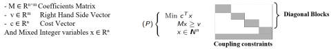
Once the problem is identified and its key components defined, we examine technical feasibility and modeling approach to solve the problem which means adapted programming methods of resolution in reasonable time. This problem is a mixed-integer linear model with too many continuous and binary variables, in addition to too many constraints. The size of the optimization problem generates a challenge for applying and maintaining such a decision model. For moderate-scale problems containing small number of binary decision variables, this planning model can be effectively resolved by commercial optimization software. However extended models intensify the magnitude and complexity of the problem. This MILP has a deterministic time-hard aspect which is supposed to be a large-scale problem as it considers different new real-world aspects of military and humanitarian supply chains.
For this problem, several MILP formulations use different variables. So, to facilitate its resolution and find out the optimal or near-optimal solution, we will oversee good reformulation changing the variable space of a problem before evaluating its quality or potential depending on:
• the obtained relaxation value: If it allows an improvement to the previous formulation, whenever approaching the integer optimum, the formulation is more likely to perform well in a branching algorithm.
• the efficient possibilities of branch techniques: avoiding the presence of too many symmetric solutions, with the same cost and/or quasi-similar structures.
• the formulation structure: when a program can be almost decoupled into independent sub-programs. Decomposition techniques make it possible to use this structure to construct particular algorithmic principles.
Most performing solutions approaches consist generally of Danzig-Wolfe decomposition and column generation to deal with too many variables, Bender’s decomposition for problem with too many constraints [46], or Lagrangian relaxation [79].
Considering the MILP (P) defined with the following Vectors and Matrixes, in practical problems, the coefficients matrix M has often the block-diagonal structure of Figure 10 where the gray areas represent the non-zero coefficients, sometimes after simultaneous permutations of rows and columns. While the bottom block represents the coupling constraints and concerns all the variables of the problem, the other diagonal blocks are smaller and concern only a limited batch of variables where they appear exclusively.
Figure 10. Coefficients matrix structure
Many authors solved IPDP without using this matrix composition, coordinating simultaneously the optimization of inventory, production and delivery, and routing in a single model. But, lots of times, this difficult approach couldn’t be resolved or blocked many times, pushing analysts to the decomposition methods that use these multiple blocks to solve it by dividing the resolution into several programs and subprograms. The master problem obtained from the original one, which gives the resolution of the initial problem, generally abides with coupling constraints and ensures a pilot role in the decomposition technique. Besides, satellite sub-problems help finalize solving the whole problem and are most often connected with the isolated blocks of the coefficients’ matrix M. The entire master program and satellite programs are then integrated into an algorithmic process converging to a lower bound or to the optimal solution of the problem. The Lagrangian duality gives a motivating setting for relaxation and decomposition. Relaxation often offers very good relaxation value, habitually better than continuous relaxation. Furthermore, a dedicated study is frequently required for the implementation of decomposition techniques that pave the way for great success on very large industrial problems.
Many scientists as Adulyasak et al. [46] reviewed existing formulations, decomposition methods and solution algorithms for inventory, production and distribution problems, discussing not only Lagrangian Relaxation, Lower bound, and Branch and Cut techniques but also exact methods, heuristics, stochastic, fuzzy optimization. Highlighting modern research findings, Ioannis [80] offered some interesting methods and resources to model and solve supply chain management problems, which propose adapted efficient and effective algorithms. In this section, this article summarizes and discusses the useful formulations, reformulations, and solution techniques for our integrated supply chain cost minimization problem IPDP, along with algorithmic and computational issues.
5.1 Approaches to compute lower bounds
In general, the IPDP is a complex combinatorial optimization problem with too many variables and constraints. Normally, the lower bound of the basic IPDP formulation attained through the resolution of the LP relaxation is not of good quality. Nananukul [47] demonstrated in his doctoral thesis that the LP relaxation is not suitable for offering relaxed solutions in exact algorithms (e.g. branch-and-bound) or in finding further near-solution methods’ quality. Therefore, they investigated substitutes for these relaxation methods to handle complexity and get better lower bounds. It concerns Lagrangian Relaxation techniques illustrated by Fisher [25], Fumero and Vercellis [43], then Solyali and Süral [52], or Column Generation approaches by Nananukul [47] and Lübbecke and Desrosiers [81], as detailed in Appendix.
5.2 Decoupled versus integrated solution method
As the IPDP embraces the structure of the LSP and Distribution or VRP problems, it is useful to give a summary of the different formulations and promising reformulations for these two problems. Pochet and Wolsey [82] highlighted the weakness of the basic LSP formulation with poor quality lower bounds. Many reformulations have been used to strengthen it, including the shortest path [83] and facility location [84] ones. Hence, both of these formulations possess the property of integrality in the case of single-level incapacitated LSP, and feasible mixed-integer solutions are attained through solving the relaxed Linear Programming (LP) formulation. Ruokokoski et al. confirmed the efficiency of multiple Lot sizing reformulations in the IPDPs. In the Distribution or VRP, many formulations are investigated to find solutions to the problems with diverse features [48]. While a classical simple formulation is appropriate for a homogeneous fleet and reduced quantity of vehicles, a developed formulation should be employed to manage a heterogeneous fleet with different numbers of transporters, consumption or costs, including vehicle indexation and multi-commodity flow consideration. This mathematical method is also normally formulated as the master problem in a column generation technique. Like in the distribution problems, some models were included in the IPDP to handle specific issues, such as the use of vehicle indexation in formulation considering a heterogeneous fleet by Lei et al. [49], and the path-based approach in the column generation method [47, 50, 51].
Regarding the integrated approach, we found out that the contributions of Chandra and Fisher [42] and Lei et al. [65] offered inspiring integrated solution approaches for our problem. Lei et al. [65] considered the integrated Production, Inventory, and Distribution Routing cost minimization Problem (PIDRP), aligning production, inventory, and delivery operations to satisfy customer demand most efficiently. It also includes heterogeneous vehicles with non-instantaneous traveling times and several client demand locations with different inventory capacities. Due to its combinatorial nature, it was hard for them to optimally solve such an integrated problem especially when vehicle routing is included; and used a two-phase solution approach. Stage I solved a mixed-integer program addressing all the constraints in the initial model but restricting distribution to direct shipments between facilities and demand points. The optimal solution they get in stage I is most of the time feasible to the original model. Stage II deepened the opportunity of a delivery consolidation problem, modeled as a capacitated transportation problem with supplementary constraints and addressed using a heuristic method.
This two-phase approach is unique as it gives the huge opportunity of coordinating simultaneously the production, inventory, and transportation functions throughout the whole planning horizon, without aggregating the demand or relaxing the constraints on transportation capacities. It is a virtuous paradigm shift from the other classical decoupled approach that optimizes separately even successively the production lot sizes before the distribution problem. This enabled them to rapidly pinpoint a high-quality suboptimal solution to the original complex problem and correct this suboptimality through the consolidation effort of stage II. The structural and performance assessment of this proposed two-phase approach shows its effectiveness and encourages our interest in this integrating method to enrich our developed model and facilitate its application to real-world supply chain networks.
In their coordinated inventory, production and distribution planning, Chandra and Fisher compared two management approaches to this system. In the first method, the production scheduling and vehicle routing problems are addressed distinctly, and in the next one, the coupled method, they are integrated within a single model. Computational results highlighted that the coupled model offers potential savings of 5 to 20% [42].
5.3 Inspiring optimization solvers
Once we have built our closed-loop multi-period multi-echelon inventory, production and distribution mathematical model aiming at minimizing the integrated supply chain cost, we will thrive to solve our complex MIP problem through a synergic prescriptive analytics approach. It combines the abovementioned simplifying reformulation technique with powerful commercial optimization software taking advantage of recent and developing computer technology improvements. The recent tremendous improvement of commercial optimization solvers, along with seeking almost the best compatibility between the appropriate solver and the analyzed model can significantly upsurge our capacity to compute satisfactory solutions to various problems with solvers like CPLEX, GUROBI, and IBM Optimization Solutions and Library (OSL) solver.
However, some recent software like General Algebraic Modeling System (GAMS) and LINGO, annually extended and enhanced, offer high-level model development environments that support the analysis and solution of an extensive range of optimization problems with a significant worldwide user base.
In our study, after simplified reformulation, we will use LINGO thanks to its flexibility, modeling language, and especially its treatment capacity, emphasized by both Hillier and Lieberman [85], and Sithole et al. [86], through the following points:
Hence, the last version of LINGO demonstrated lately to be a comprehensive modeling language and optimizer with high performance in building (including data codification) and solving large-scale Linear, Nonlinear (convex, non-convex / Global), Quadratic, Quadratically Constrained, Second Order Cone, Semi-Definite, Stochastic, and Integer optimization models faster, easier and more efficiently [86, 75].
The optimization of the proposed closed-loop multi-period multi-echelon supply chain consists of minimizing the total cost of inventory and back-orders, production and distribution functions from support facilities to all non-stationary demand points over T periods within a determined Satisfaction Performance Level (SPL). The general structure of the considered network can be applied to different kinds of humanitarian and military organizations, as well as to vehicle and electronic industries. Getting informed of 72 past and recent studies by well-known specialized scientists and professionals, the obtained results of this literature review and gaps findings demonstrate the originality of the contribution of the proposed work to the scientific research community. These integrating models are garnering increasing global attention as contemporary society, institutions, and governments recognize more acutely not only the critical importance of this knowledge for survival but also for its sustainable economic value. The problem formulation of the model led to a challenging MINLP problem, with too many variables and constraints. Some possible solutions are proposed to illustrate such an integrated approach, which can be improved in future research through risk pooling and uncertainty mitigation to face attritions of real-world environments.
Having reviewed and classified related literature works based on problem characteristics, supply chain structure, objective, modeling approach, decision variables and solution methods, the purpose of this study consists also of describing and proposing an optimal push-pull integrated inventory-production-distribution model with a discussion of potential solution methods (reformulation, branching and relaxation) and promising LINGO algorithms. It is a prelude to their future application and computation for results validation and outcomes comparison with the standard push supply chain model. This prescriptive analysis introduces a model that empowers decision-makers to simultaneously optimize product and customer allocations, fleet size and inventory holding within a multi-echelon, multi-period, multi-commodity forward/reverse supply chain system. The problem formulation of the model led to a challenging MILP problem, with too many variables and constraints. Some possible solution methods are proposed to illustrate such an integrated approach.
A comparative study of LINGO integrated and decoupled approaches’ outputs of the model would be an interesting avenue of reflection, that can be extended with predictive analytics, especially demand forecasting like the Mamdani-fuzzy logic decision model just recently proposed by three authors of the present article in [87] and last-mile logistics [88]. Indeed, we point out stimulating research perspectives that can enhance the proposed supply chain planning model, including sustainability-based risk pooling [89] and fuzzy optimization to satisfy and adapt scenario-based demand for uncertainty mitigation in a real-world environment. By switching from consumption-based deterministic to fuzzy demand considering simultaneously the three relevant indicators of Consumption Severity, Market Sensitivity, and Commodity Importance, the integration of Artificial Intelligence would provide dynamic visibility and efficiency into volatile supply chain operations.
|
IPDP |
Inventory-Production-Distribution Problem |
|
SC |
Supply Chain |
|
CRSC |
Crisis Relief Supply Chain |
|
MILP |
Mixed Integer Linear Programming Model |
|
Sets and Indices |
|
|
T |
Set of time-periods; |
|
K |
Set of classes of commodities; |
|
S, J |
Set of Source Supplier and Warehouses (or ISF); |
|
N |
Set of demand locations associated with respective intermediate support facilities (Warehouses); |
|
V |
Set of vehicles of class v (transportation resource) e.g: 5 Tons Cargo Truck, 6 Tons Tank Truck, etc.; |
|
Kv |
Set of commodities classes compatible with vehicle of class v∈V; |
|
O |
Set of maintenance workforce (or resources); |
|
G, M, C, Q |
Set of costs successively for Inventory Holding, Production, Transportation and Shortage Penalty. |
|
Parameters |
|
|
Dnjkt |
Demand for commodity k from demand location n to intermediate support facility j (Pallets), in period t; |
|
α, β |
Demand satisfaction rate or level, lowest possible limit, such as 0<β≤α≤1; |
|
wk |
Weight of a unit of commodity k (Tons/Pallet); |
|
zv |
Payload capacity of a transportation vehicle of class v (Tons); |
|
Uik |
Inventory holding capacity of commodity k at intermediate support facility s (Pallets); |
|
Usv |
Transportation capacity on vehicles of class v at source support facility s (Tons); |
|
Ujv |
Transportation capacity on vehicles of class v at intermediate support facility j (Tons); |
|
Upj |
Maintenance capacity at intermediate support facility j (Hours); |
|
zo |
Workforce capacity of a maintainer o (Hours); |
|
ajkt |
Amount of workforce necessary for maintenance of a unit of commodity k at support facility j (Hrs/Pallet): a unit of weapon or automotive system is considered as 1 pallet of commodity k=2 (k’); |
|
hkv |
=1 when k∈Kv, 0 otherwise. This indicator parameter signifies the compatibility between the class of commodity k and the class of vehicle v; |
|
Lvs, Lvj |
Number of vehicles of class v∈V successively at SSF S and ISF j∈J. |
|
Rnjkvt |
Reverse shipment quantity of defective commodity k from Customer n to ISF j on vehicle v in period t (note that ckfnt=cknft); |
|
γvkk' |
=1 if commodities classes k∈K, k’∈K, k≠k’, can be shipped together (on the same vehicle, at the same time) by vehicle of class v; 0 otherwise; |
|
gsk |
Unit inventory holding cost for commodity k at source support facility s ($/Pallet); |
|
gjk |
Unit inventory holding cost for commodity k at intermediate support facility j ($/Pallet); |
|
csjkt |
Unit transportation cost for shipment of commodity k from source s to intermediate support facility j ($/Pallet) in period t: length sj*fuel consumption of v*consumed fuel cost |
|
cjnkt |
Unit transportation cost for shipment of commodity k from intermediate support facility j to demand location n ($/Pallet) in period t: same for length jn; |
|
cnjkt |
Unit transportation cost for reverse recovery of commodity k from demand location n to intermediate support facility j ($/Pallet) in period t, be it known that cnjk=cjnk; |
|
mjkt |
Unit maintenance cost for commodity k at intermediate support facility j ($/Pallet) in period t; |
|
qjkt |
Unit shortage penalty cost for not satisfying customer demand of commodity k at intermediate support facility j ($/Pallet) in period t. |
Detailing of lagrangian relaxation and column generation optimization methods
(1). Lagrangian relaxation
Fisher simplified the concept of Lagrangian relaxation, as a method to acquire lower bounds by dualizing constraints with Lagrangian multipliers and splitting the model into more tractable sub-problems. Indeed, it is often useful to use a decomposition approach in some mixed-integer programs with a nice structure of the sub-set of constraints. More probably, a Lagrangian technique offers a stronger bound, that may be more interesting in branch-and-bound algorithms, compared to those obtained through the standard LP relaxation solution approach.
To find out potential solution approaches that would fit our proposed model, we surveyed the outcomes of Lagrangian relaxation in a range of IPDP optimization problem variants. Fumero and Vercellis used Lagrangian relaxation (LR) to solve a multi-period cost minimization MIP of production and logistics operations where unit transportation costs are considered. Computational results on various sizes’ tests and the algorithm point out a great advantage of the synchronized technique over the decoupled method where a production plan (LSP) is formulated followed by the subsequent resolution of a distribution schedule (VRP). They use a reformulation approach dualizing the plant inventory constraints and the vehicle capacity constraints. Applications with up to 8 periods, 12 customers and 10 products give an average gap of 5.5% better. The Lagrangian relaxation applied within the integrated model obtains both lower bounds and heuristic feasible solutions more effective than that found by the alternative decomposed decision process. Nonetheless, the use of an almost similar Lagrangian relaxation technique by Solyali and Süral to solve the IPDP with the order-up-to-level (OU) policy, gives weaker lower bounds compared to the Fumero and Vercellis’ results [utilizing the unit transportation costs.
(2). Column generation
To handle the complexity of combinatorial IPDP optimization problems, the column generation approach offers rewarding results. The decomposition of a principal formulation into a restricted master problem (RMP) and subproblems is improved through the replacement of original variables with a convex combination of extreme points of the subproblems, generated and incorporated progressively through the iterative resolution of the subproblems. Lübbecke and Desrosiers detailed recent column generation applications to integrated supply chain problems. Among investigated papers, Nananukul elaborated a mixed-integer programming (MIP) model aiming at minimizing the total cost of production, inventory, and distribution throughout the various stages of the supply chain. He formulated an RMP and subproblem for the IPDP and elaborated a novel efficient column generation-based hybrid solution methodology combining exact and heuristic methods within a precise branch-and-price procedure. The author characterized the sets of delivery plans in a period by the delivery quantity to each customer and routing decisions and managed to handle symmetry, showing more effectiveness than CPLEX or standard branch-and-price alone.
[1] Christopher, M. (1999). Logistics and supply chain management. Strategies for Reducing Cost and Improving Service Financial Times. Pitman Publishing. London, 1998 ISBN 0 273 63049 0 (hardback) UK. https://doi.org/10.1080/13675569908901575
[2] Kress, M. (2002). Operational logistics. In The Art and Science of Sustaining Military Operations. Springer Cham & Kluwer Academic Publishers, USA. https://doi.org/10.1007/978-3-319-22674-3
[3] Kiley, G. (2001). The Effects of Aging on the Costs of Operating and Maintaining Military Equipment. Congressional Budget Office Paper, Congress of USA, pp. 3-4. https://apps.dtic.mil/sti/tr/pdf/ADA393973.pdf
[4] Stadtler, H., Christoph K. (2010). Supply Chain Management and Advanced Planning: Concept, Models, Software, and Case Studies (4th ed.) Springer Publishing Company. https://dl.acm.org/doi/book/10.5555/1965255
[5] Cottle, R.W. (2005). George B. Dantzig: Operations research icon. Operations Research, 53(6): 892-898. https://doi.org/10.1287/opre.1050.0250
[6] Saidi, D., El Alami, J., Hlyal, M. (2021). Building sustainable resilient supply chains in emerging economies: Review of motivations and holistic framework. In IOP Conference Series: Earth and Environmental Science. IOP Publishing. China, 690(1): 012057. https://doi.org/10.1088/1755-1315/690/1/012057
[7] Moher, D., Liberati, A., Tetzlaff, J., Altman, D.G., The PRISMA Group (2009). Preferred reporting items for systematic reviews and meta-analyses: The PRISMA statement. PLoS Medicine, 6(7): e1000097. https://doi.org/10.1371/journal.pmed.1000097
[8] Lucas, P.J., Baird, J., Arai, L., Law, C., Roberts, H.M. (2007). Worked examples of alternative methods for the synthesis of qualitative and quantitative research in systematic reviews. BMC Medical Research Methodology, 7: 1-7. https://doi.org/10.1186/1471-2288-7-4
[9] Bhatnagar, R., Chandra, P., Goyal, S.K. (1993). Models for multi-plant coordination. European Journal of Operational Research, 67(2): 141-160. https://doi.org/10.1016/0377-2217(93)90058-U
[10] Chen, F., Federgruen, A., Zheng, Y.S. (2001). Coordination mechanisms for a distribution system with one supplier and multiple retailers. Management Science, 47(5): 693-708. https://doi.org/10.1287/mnsc.47.5.693.10484
[11] Dubey, R., Bryde, D.J., Foropon, C. (2024). Design and management of humanitarian supply chains for pandemics: Lessons from COVID-19. Annals of Operations Research, 335(3): 885-898. https://doi.org/10.1007/s10479-024-05944-3
[12] Kovacs, G., Spens, K.M. (2012). Relief supply chain management for disasters: Humanitarian aid and emergency logistics. Hershey, PA: Information Science Reference. IGI Global, PA, USA. https://doi.org/10.4018/978-1-60960-824-8
[13] Zhu, J., Shi, Y., Venkatesh, V., Islam, S., Hou, Z., Arisian, S. (2022). Dynamic collaborative optimization for disaster relief supply chains under information ambiguity. Annals of Operations Research, 335: 1-27. https://doi.org/10.1007/s10479-022-04758-5
[14] Song, J.M., Chen, W., Lei, L. (2018). Supply chain flexibility and operations optimization under demand uncertainty: A case in disaster relief. International Journal of Production Research, 56(10): 3699-3713. https://doi.org/10.1080/00207543.2017.1416203
[15] Habib, M.S., Lee, Y.H., Memon, M.S. (2016). Mathematical models in humanitarian supply chain management: A systematic literature review. Mathematical Problems in Engineering, 2016(1): 3212095. https://doi.org/10.1155/2016/3212095
[16] Staff, U.J. (2000). JP 4-0 doctrine for logistics support of joint operations. Joint Doctrine Publications, US Department of Defense, USA, April 2008, III 10-13.
[17] Wilson VornDick. (2013). The Pentagon’s Logistics Nightmare. International Policy Digest, May 9, USA.
[18] NAVAIR. (2014). NAVAIR Maintenance Trade Cost Guidebook. (Ver. 2.01). Naval Air Systems Command (NAVAIR) Cost Department: Research and Engineering. Décembre 1st, USA. http://everyspec.com/USN/NAVAIR/NAVAIR_MAINTENANCE_TRADE_COST_GUIDE_V2--01_4119
[19] DGCIPA. (2019). Cost Factors Manual: Air Chapter 2018-2019. National Defense Headquarters: Centre for Costing in Defense. GC Docs 18006893. March, Ottawa, Canada. https://www.taxpayer.com/media/cost-factors-manual-2018-19-air-chapter.pdf.
[20] Sebbah, S., Ghanmi, A., Boukhtouta, A. (2011). Design of tactical strategies in military logistics: Trade-offs between efficiency and effectiveness. Defense R&D Canada DRDC CORA Technical Memorandum TM 2011-211, December.
[21] Parlier, Greg H. (2005). Transforming U.S. army logistics: A strategic “supply chain” approach for inventory management. The Land Warfare Papers, 74 (UA23.A95L16 N°54). AUSA Institute of Land Warfare, Arlington, USA. http://www.ausa.org/pdfdocs/LWP_54.pdf.
[22] Dantzig, G.B., Orchard-Hays, W. (1954). The product form for the inverse in the simplex method. Mathematical Tables and Other Aids to Computation, 64-67. https://doi.org/10.1090/S0025-5718-1954-0061469-8
[23] Dantzig, B.G. (2002). Linear programming. Operations Research, INFORMS, 50(1): 42-47. https://doi.org/10.1287/opre.50.1.42.17798
[24] Graves Stephen, C. (2014). Inventory Management: Deterministic-demand Inventory Models. MIT Open Course Ware, 15.772J / EC.733J D-Lab: Supply Chains., Lecture 13, Fall. MIT Sloan, Massachusetts, USA. https://ocw.mit.edu/courses/15-772j-d-lab-supply-chains-fall-2014/resources/mit15_772jf14_lec13/.
[25] Fisher, M.L. (1981). The Lagrangian relaxation method for solving integer programming problems. Management Science, 27(1): 1-18. https://doi.org/10.1287/mnsc.27.1.1
[26] Archetti, C., Bertazzi, L., Paletta, G., Speranza, M.G. (2011). Analysis of the maximum level policy in a production-distribution system. Computers & Operations Research, 38(12): 1731-1746. https://doi.org/10.1016/j.cor.2011.03.002
[27] Santany, M. (2015). Exploring the influences of relational competencies on supply chain agility. International Journal of Applied Engineering Research, 10(19): 40566-40574. https://www.ripublication.com/ijaer10/ijaerv10n19_116.pdf.
[28] Shapiro, J.F. (2001). Modeling the Supply Chain. Duxbury Press, Pacific Grove, CA, USA. p. 586. https://fr.scribd.com/document/504412634/Modeling-the-Supply-Chain.
[29] Berbiche, N., Hlyal, M., El Alami, J. (2020). Exponential success through integrated supply chain optimization, ecomotional intelligence and reputation-based leadership: Zara model. In IOP Conference Series: Materials Science and Engineering. IOP Publishing, 827(1): 012058. https://doi.org/10.1088/1757-899X/827/1/012058
[30] Maleki, M., Cruz-Machado, V. (2013). A review on supply chain integration: Vertical and functional perspective and integration models. Economics and Management, 18(2): 340-350. https://doi.org/10.5755/j01.em.18.2.2968
[31] Hillier, F.S., Lieberman, G. (2001). Introduction to Operations Research, (7th ed) McGraw Hill Education, Dubuque, Iowa, USA. https://archive.org/details/introduction-to-operations-research/page/n5/mode/2up.
[32] Jayaraman, V., Guide Jr, V.D.R., Srivastava, R. (1999). A closed-loop logistics model for remanufacturing. Journal of the Operational Research Society, 50(5): 497-508. https://doi.org/10.1057/palgrave.jors.2600716
[33] Fleischmann, M., Beullens, P., Bloemhof-Ruwaard, J.M., Van Wassenhove, L.N. (2001). The impact of product recovery on logistics network design. Production and Operations Management, 10(2): 156-173. https://doi.org/10.1111/j.1937-5956.2001.tb00076.x
[34] Tafaghodi, K., Seyed, M., Seyed, H., Makui, A. (2011). A mathematical model for optimization of an integrated network logistics design. Management Science Letters, 1, Growing Science Ltd., 415-426. http://doi.org/10.5267/j.msl.2011.05.003
[35] Letchford, A.N., Salazar-González, J.J. (2006). Projection results for vehicle routing. Mathematical Programming, 105: 251-274. https://doi.org/10.1007/s10107-005-0652-x
[36] Min, H., Jayaraman, V., Srivastava, R. (1998). Combined location-routing problems: A synthesis and future research directions. European Journal of Operational Research, 108(1): 1-15. https://doi.org/10.1016/S0377-2217(97)00172-0
[37] Hlyal, M., Ait Bassou, A., Soulhi, A., El Alami, J., El Alami, N. (2015). Designing a distribution network using a two level capacity location allocation problem: Formulation and efficient genetic algorithm resolution with an application to a moroccan retail company. Journal of Theoretical & Applied Information Technology, 72(2): 294-306.
[38] Bassou, A.A., Hlyal, M., Soulhi, A., El Alami, J. (2016). New variable neighborhood search method for a two level capacitated location allocation problem. Journal of Theoretical and Applied Information Technology, 83(3): 442-445.
[39] Chekoubi, Z., Trabelsi, W., Sauer, N. (2018). The integrated production-inventory-routing problem in the context of reverse logistics: The case of collecting and remanufacturing of EOL products. In 2018 4th International Conference on Optimization and Applications (ICOA), Mohammedia, Morocco, pp. 1-6. https://doi.org/10.1109/ICOA.2018.8370563
[40] Devangan, L.K. (2016). An integrated production, inventory, warehouse location and distribution model. Journal of Operations and Supply Chain Management, 9(2): 17-27.
[41] Chen, A. (2014). Inventory management: Stochastic-demand Inventory Models, Part II. MIT Open Course Ware, 15.772J / EC.733J. D-Lab: Supply Chains, Lecture 14, MIT Sloan, Massachusetts, USA, Fall. https://ocw.mit.edu/courses/15-772j-d-lab-supply-chains-fall-2014/resources/mit15_772jf14_lec14/.
[42] Chandra P., Fisher, M.L. (1994). Coordination of production and distribution planning. European Journal of Operational Research, 72(3): 503-517. https://doi.org/10.1016/0377-2217(94)90419-7
[43] Fumero, F., Vercellis, C. (1999). Synchronized development of production, inventory, and distribution schedules. Transportation Science, 33(3): 330-340. https://doi.org/10.1287/trsc.33.3.330
[44] Archetti, C., Bertazzi, L., Laporte, G., Speranza, M.G. (2007). A branch-and-cut algorithm for a vendor-managed inventory-routing problem. Transportation Science, 41(3): 382-391. https://doi.org/10.1287/trsc.1060.0188
[45] Solyali, O., Sural, H. (2011) A branch-and-cut algorithm using a strong formulation and an a priori tour-based heuristic for an inventory-routing problem. Transportation Science, 45(3): 335-345. https://doi.org/10.1002/nav.20428
[46] Adulyasak, Y., Cordeau, J.F., Jans, R. (2015). The production routing problem: A review of formulations and solution algorithms. Computers and Operations Research, 55: 141-152. https://doi.org/10.1016/j.cor.2014.01.011
[47] Nananukul, N. (2008). Lot-sizing and inventory routing for production, inventory and distribution systems. Ph.D Thesis, Graduate Program in Operations Research and Industrial Engineering. The University of Texas, Austin, pp. 31-58. http://hdl.handle.net/2152/3960.
[48] Ruokokoski, M., Solyali, O.G.U.Z., Cordeau, J.F., Jans, R., Süral, H. (2010). Efficient formulations and a branch-and-cut algorithm for a production-routing problem. GERAD Technical Report, G-2010-66, HEC Montréal, Canada, pp. 1-43.
[49] Lei, L., Liu, S., Ruszczynski, A., Park, S. (2006). On the integrated production, inventory, and distribution routing problem. IIE Transactions, 38(11): 955-970. https://doi.org/10.1080/07408170600862688
[50] Bard, J.F., Nananukul, N. (2009). Heuristics for a multiperiod inventory routing problem with production decisions. Computers & Industrial Engineering, 57(3): 713-723. https://doi.org/10.1016/j.cie.2009.01.020
[51] Bard, J.F., Nananukul, N. (2010). A branch-and-price algorithm for an integrated production and inventory routing problem. Computers & Operations Research, 37(12): 2202-2217. https://doi.org/10.1016/j.cor.2010.03.010
[52] Solyali, O., Süral, H. (2009). A relaxation-based solution approach for the inventory control and vehicle routing problem in vendor-Managed systems. In Modeling, Computation and Optimization, World Scientific, Singapore, 171-189. https://doi.org/10.1142/9789814273510_0011
[53] Pirkul, H., Jayaraman V. (1996). Production, transportation and distribution planning in a multi-commodity tri-echelon system. Transportation Science, 30(4): 291-302. https://doi.org/10.1287/trsc.30.4.291
[54] Jayaraman, V. (2006). Production planning for closed-loop supply chains with product recovery and reuse: An analytical approach. International Journal of Production Research, 44(5): 981-998. https://doi.org/10.1080/00207540500250507
[55] Jayaraman, V., Pirkul, H. (2001). Planning and coordination of production and distribution facilities for multiple commodities. European Journal of Operational Research, 133(2): 394-408. http://doi.org/10.1016/S0377-2217(00)00033-3
[56] Noyan, N., Balcik, B., Atakan, S. (2016). A stochastic optimization model for designing last mile relief networks. Transportation Science, 50(3): 1092-1113. https://doi.org/10.1287/trsc.2015.0621
[57] Minic, S.M., Gendreau, M., Potvin, J.Y., Berger, J., Conrad, J., Thomson, D. (2014). Three-echelon supply chain management for disaster relief operations. CIRRELT, Interuniversity Research Centre on Enterprise Networks, Logistics and Transportation. Quebec, Bibliothèque et Archives Canada.
[58] Doyen, A., Aras, N., Barabarosoglu, G. (2011). A two-echelon stochastic facility location model for humanitarian relief logistics. Optimization Letters, 6: 1123-1145. https://doi.org/10.1007/s11590-011-0421-0
[59] Özdamar L., Yazgac, T. (1999). A hierarchical planning approach for a production-distribution system. International Journal of Production Research, 37(16): 3759-3772. https://doi.org/10.1080/002075499190031
[60] Forma, I., Raviv, T., Tzur, M. (2009). Functional decompositions for a production and distribution system. IFAC Proceedings Volumes, Moscow, Russia, June 3-5, 42(4): 1268-1273. https://doi.org/10.3182/20090603-3-RU-2001.0415
[61] Qu, W.W., Bookbinder, J.H., Iyogun, P. (1999). An integrated inventory-transportation system with modified periodic policy for multiple products. European Journal of Operational Research, 115(2): 254-269. https://doi.org/10.1016/S0377-2217(98)00301-4
[62] Federgruen, A., Tzur, M. (1999). Time‐partitioning heuristics: Application to one warehouse, multiitem, multiretailer lot‐sizing problems. Naval Research Logistics (NRL), 46(5): 463-486. https://doi.org/10.1002/(SICI)1520-6750(199908)46:5%3C463:AID-NAV2%3E3.0.CO;2-S
[63] Berman, O., Wang, Q. (2007). Inbound logistic planning: Minimizing transportation and inventory costs. Transportation Science, 40(3): 287-299. https://doi.org/10.1287/trsc.1050.0130
[64] Toptal, A., Çetinkaya, S. (2008). Quantifying the value of buyer–vendor coordination: Analytical and numerical results under different replenishment cost structures European Journal of Operational Research, 187: 785-805. https://www.sciencedirect.com/science/article/abs/pii/S0377221706007831?via%3Dihub.
[65] Lei, L., Liu, S., Ruszczynski, A., Park, S. (2006). On the integrated production, inventory, and distribution routing problem. IIE Transactions, 38(11): 955-970. https://doi.org/10.1080/07408170600862688
[66] Amin, S.H., Zhang, G. (2012). A proposed mathematical model for closed-loop network configuration based on product life cycle. The International Journal of Advanced Manufacturing Technology, 58: 791-801. https://doi.org/10.1007/s00170-011-3407-2
[67] Fleischmann, M., Bloemhof-Ruwaard, J.M., Dekker, R., Van der Laan, E., Van Nunen, J.A., Van Wassenhove, L.N. (1997). Quantitative models for reverse logistics: A review. European Journal of Operational Research, 103(1): 1-17. https://doi.org/10.1016/S0377-2217(97)00230-0
[68] Jamsa, P. (2009). Opportunities for research in reverse logistics networks: A literature review. International Journal of Management and Enterprise Development, 6(4): 433-454. https://doi.org/10.1504/IJMED.2009.024234
[69] Rubio, S., Chamorro, A., Miranda, F.J. (2008). Characteristics of the research on reverse logistics (1995-2005). International Journal of Production Research, 46(4): 1099-1120. https://doi.org/10.1080/00207540600943977
[70] Jayaraman, V. (1998). Transportation, facility location and inventory issues in distribution network design: An investigation. International Journal of Operations and Production Management, 18(5): 471-494. https://doi.org/10.1108/01443579810206299
[71] Jayaraman, V., Patterson, R., Rolland, E. (2003). The design of reverse distribution networks: Models and solution procedures. European Journal of Operational Research, 150(1): 128-149. https://doi.org/10.1016/S0377-2217(02)00497-6
[72] Salema, M.I.G., Barbosa-Povoa, A.P., Novais, A.Q. (2007). An optimization model for the design of a capacitated multi-product reverse logistics network with uncertainty. European Journal of Operational Research, 179(3): 1063-1077. https://doi.org/10.1016/j.ejor.2005.05.032
[73] Salmerón, J., Apte, A. (2010). Stochastic optimization for natural disaster asset prepositioning. Production and Operations Management, 19(5): 561-574. https://doi.org/10.1111/j.1937-5956.2009.01119.x
[74] Ozdamar, L. (2017). Disaster relief logistics. In Wiley StatsRef: Statistics Reference Online. John Wiley & Sons, Chichester. http://doi.org/10.1002/9781118445112.stat08019
[75] Guide Jr., D.R., Van Wassenhove, L.N. (2009). The evolution of closed-loop supply chain research. Operations Research, 57(1): 10-18. https://doi.org/10.1287/opre.1080.0628
[76] Gilmore, P.C., Gomory, R.E. (1993). A linear programming approach to cutting stock problem (Part II). Operations Research, 11: 363-888.
[77] Abou-El-Seoud, N., Howell, R. (2012). Redefining the future of tactical equipment maintenance facilities: new multifunctional maintenance complexes to meet 21st century demands. US Army Sustainment, 44: 52-55.
[78] Üster, H., Easwaran, G., Akçali, E., Çetinkaya, S. (2007). Benders decomposition with alternative multiple cuts for a multi‐product closed‐loop supply chain network design model. Naval Research Logistics (NRL), 54(8): 890-907. https://doi.org/10.1002/nav.20262
[79] Fisher, M.L. (1985). An applications-oriented guide to Lagrangian Relaxation. Interfaces, 15(2): 10-21. https://doi.org/10.1287/inte.15.2.10
[80] Ioannis, T.C. (2013). Quantitative methods in supply chain management: Models and algorithms. Springer London: UK, pp. 102-281.
[81] Lübbecke M.E., Desrosiers, J. (2005). Selected topics in column generation. Operations Research, 53(6): 1007-1023. https://doi.org/10.1287/opre.1050.0234
[82] Pochet Y., Wolsey, L.A. (2006). Single-item incapacitated lot-sizing. In Production Planning by Mixed Integer Programming: Chapter 7. Springer Series in Operations Research and Financial Engineering, Springer: New York, 207-234. https://books.google.co.ma/books?id=Uv8vn_kQZqEC&printsec=frontcover#v=onepage&q&f=false.
[83] Eppen G.D., Martin, R.K. (1987). Solving multi-item capacitated lot-sizing problems using variable redefinition. Operations Research, 35(6): 832-848. https://doi.org/10.1287/opre.35.6.832
[84] Krarup, J., Bilde, O. (1977). Plant location, set covering and economic lot size: An 0 (mn)-algorithm for structured problems. Numerische Methoden bei Optimierungsaufgaben Band 3: Optimierung bei Graphentheoretischen und Ganzzahligen Problemen, Birkhäuser, Basel, 155-180. https://doi.org/10.1007/978-3-0348-5936-3_10
[85] Hillier F., Lieberman G. (2021). Introduction to Operations Research, 11th Ed. McGraw Hill, USA.
[86] Sithole, B., Silva, S.G., Kavelj, M. (2016). Supply chain optimization: Enhancing end-to-end visibility. Procedia Engineering, 159: 12-18. https://doi.org/10.1016/j.proeng.2016.08.058
[87] Berbiche, N., Hlyal, M., El Alami, J. (2024). Enhancing supply chain resilience and efficiency through fuzzy logic-based Decision-Making automation in volatile environments. Ingénierie des Systèmes d'Information, 29(1): 191-203. https://doi.org/10.18280/isi.290120
[88] Cooper, M. and Ellram, L. (1993). Characteristics of Supply Chain Management and the Implications for Purchasing and Logistics Strategy. The International Journal of Logistics Management. 4(2): 13-24. https://doi.org/10.1108/09574099310804957
[89] Saidi, D., El Alami, J., Hlyal, M. (2020). Sustainable supply chain management: Review of triggers, challenges and conceptual framework. In IOP Conference Series: Materials Science and Engineering. IOP Publishing, 827(1): 012054. https://doi.org/10.1088/1757-899X/827/1/012054