Abdullah Mohammed Yahia*![]() | Ahmed Alkamachi
| Ahmed Alkamachi![]()
© 2024 The authors. This article is published by IIETA and is licensed under the CC BY 4.0 license (http://creativecommons.org/licenses/by/4.0/).
OPEN ACCESS
The mathematical model for a full actuated T-shaped Tri-copter is derived in details and a suitable controller is proposed in this work. The system is governed by three tiltable motor– propeller sets to change the thrust direction to a desired angle. This will lead to the achievement of maneuverability and reduce power consumption. To control the model, a feedback linearization method is used to decouple and get a direct control on the copter degree of freedoms. Attitude and Altitude PID controller is designed to control the system and fulfil the desired trajectory. The PID parameters are tuned using Genetic algorithm (GA) optimization method. The system and the controller performance are proved using MATLAB Simulink platform through several flight scenarios.
UAV, Tri-copter, thrust vectoring, PID, genetic algorithm, feedback linearization
The unmanned aerial vehicles (UAVs) have proven their reliability and capability in many fields during the past few years, hence they come in different shapes and designs to meet the full requirement of their design purpose [1].
Tri-copters commonly come in two shapes (Y) and (T) and the rotors are located at the free end of each arm. The most common problem with tri-copter is the yawing problem which is caused by unpaired or asymmetrical locations placing of propellers. This problem can be overcome using co-axial rotors [2], manipulating propeller speeds [3], or by controlling the propeller thrust direction [4, 5]. Thrust vectoring has a benefit of stabilizing and boosting the tri-copter speed and acceleration and it can be achieved by adding a specific mechanism using a servo motor in different configurations [4-6].
Tiltable tri-rotors UAVs are the most efficient regarding power consumption, compact design, and agility [7]. Yet, it can be challenging in control means, therefore the researchers have verified many models and control techniques in that field. For example, a nonlinear (H∞) filter is developed in study [8], an LQR controller is implemented in study [9], a neural network is used to control the UAV in study [10], and the most common control method is PID controller [11]. Several optimization methods are used to adjust the PID controller parameters used in the tri-copter. For example, grey wolf optimization is used in study [12], particle swarm optimization (PSO) is used in study [13], genetic algorithm is also implemented in that aspect in studies [14, 15].
The power consumption of UAVs can be a problem in long-term flights which is reduced in tri-copters [16] and it can be further improved and give better performance if it is combined with propeller vectoring [17].
In this paper, a T-shaped Tri-rotor UAV with a tilting mechanism for each rotor is proposed. The proposition is going through modeling and controlling the UAV using feedback linearization and a PID controller. T shape was chosen because it is easy to assemble and have higher strength rating [18].
The main contributions of this work are: (1) To derive a complete dynamic model for the T-shaped Tri-copter with tiltable propellers, (2) To design a control system using PID with feedback linearization, (3) to optimize the PID performance with optimization algorithm and test its results.
The paper consists of 5 sections. We have been through section (1) introduction, section (2) is about the mathematical model of the UAV, section (3) the control system which includes feedback linearization and PID algorithm, section (4) discusses the simulation results. Finally, in section (5) the conclusion of this paper is presented.
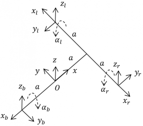
In this section, the mathematical equations that represent forces, torque, and drag torque acting on the UAV are represented. The schematic drawing of the drone along with the acting axes are shown in Figure 1.
Figure 1. Tri-rotors UAV schematic
The parameters of the UAV are cited from the study [19] as a prototype model and are shown in the Table 1.
Table 1. Tri-rotors UAV parameters
|
Parameter |
Description |
Value |
|
$m$ |
UAV mass |
2.3 kg |
|
$a$ |
Arm length |
0.3 m |
|
$I_{x x}$ |
Body inertia of x axis |
8.04 × 10⁻³ kg.m2 |
|
$I_{y y}$ |
Body inertia of y axis |
8.46 × 10⁻³ kg.m2 |
|
$I_{z z}$ |
Body inertia of z axis |
14.68 × 10⁻³ kg.m2 |
|
$k_f$ |
Force coefficient |
5 × 10⁻² N.s2 |
|
$k_t$ |
Torque coefficient |
5 × 10⁻⁴ N.m.s2 |
2.1 Forces
There are four forces acting on the UAV: the forces produced by three rotors and the gravitational force.
2.1.1 Rotors produced forces
The individual forces produced by each rotor can be written as shown below:
$f_{p_{(\cdot)}}=\left[\begin{array}{c}0 \\ k_f \omega_{m_{(\cdot)}}^2 sin \left(\alpha_{(\cdot)}\right) \\ k_f \omega_{m_{(\cdot)}}^2 cos \left(\alpha_{(\cdot)}\right)\end{array}\right]$ (1)
where, $\omega_{\mathrm{m}_{(.)}}$ is the is the rotational speed and $\alpha_{(.)}$ is the tilting angle of the corresponding motor where (.) represent the corresponding letter for each arm (l) for left arm, (r) for right and (b) for back arm.
The forces acting on the center of mass COM (O) are:
$f_{p_{(.)}}^o=R_{(.)}^o f_{p_{(.)}}^{(.)}$ (2)
The general form for the rotation matrix from the local coordinates to the O coordinate is:
$R$=$\left[\begin{array}{ccc}C_\theta C_\psi & C_\theta S_\psi & -S_\theta \\ -C_\phi S_\psi+S_\phi S_\theta C_\psi & C_\phi C_\psi+S_\phi S_\theta S_\psi & S_\phi C_\theta \\ S_\phi S_\psi+C_\phi S_\theta C_\psi & -S_\phi C_\psi+C_\phi S_\theta S_\psi & C_\phi C_\theta\end{array}\right]$ (3)
where, $C_{()}, S_{()}$ is the cosine and sine function respectively.
From Figure 1, the $\theta, \,\,\phi,$ and $\psi$ are taken as:
From $r$ to O: $\phi_r=0, \,\,\theta_r=0$ and $\psi_r=90$.
From $l$ to O: $\phi_l=0, \,\,\theta_l=0$ and $\psi_l=-90$.
From $b$ to O: $\phi_b=0,\,\, \theta_b=0$ and $\psi_b=180$.
$R_r^o=\left[\begin{array}{ccc}0 & 1 & 0 \\ -1 & 0 & 0 \\ 0 & 0 & 1\end{array}\right]$ (4)
$R_l^o=\left[\begin{array}{ccc}0 & -1 & 0 \\ 1 & 0 & 0 \\ 0 & 0 & 1\end{array}\right]$ (5)
$R_b^o=\left[\begin{array}{ccc}-1 & 0 & 0 \\ 0 & -1 & 0 \\ 0 & 0 & 1\end{array}\right]$ (6)
The summation of the forces can be written as:
$\sum f_p^o=f_{p_r}^o+f_{p_l}^o+f_{p_b}^o$ (7)
$\begin{gathered}f_p^o= {\left[\begin{array}{c}k_f \omega_{m_r}^2 sin \left(\alpha_r\right)-k_f \omega_{m_l}^2 sin \left(\alpha_l\right) \\ -k_f \omega_{m_b}^2 sin \left(\alpha_b\right) \\ k_f \omega_{m_r}^2 cos \left(\alpha_r\right)+k_f \omega_{m_l}^2 cos \left(\alpha_l\right)+k_f \omega_{m_b}^2 cos \left(\alpha_b\right)\end{array}\right]}\end{gathered}$ (8)
2.1.2 Gravitational force
The gravitational force in earth coordinates system is:
$f_g^e=\left[\begin{array}{c}0 \\ 0 \\ -m g\end{array}\right]$ (9)
and the gravitational force in (O) coordinate system is:
$f_g^o=R_e^o f_g^e$ (10)
By multiplying the gravitational force with rotation matrix in Eq. (3). (earth to O).
$f_g^o=m g\left[\begin{array}{c}S_\theta \\ -S_\phi C_\theta \\ -C_\phi C_\theta\end{array}\right]$ (11)
2.2 Torques
There are two types of torques produced by each rotor the torque produced by the lifting force of the rotors and the drag torque that is produced by the aerodynamic force acting on the propeller’s blades in the opposite direction of the rotation.
2.2.1 Rotors torques
The torque acting on the COM of the UAV can be described by:
$\tau_{p_{(.)}}^o=l_{(.)}^o \times f_{p_{(.)}}^o$ (12)
where $l_{(.)}^o$ is a vector that represent the position of the propeller in COM coordinates O, and $\times$ referes to a cross product. Therefore, the total torque acting on O is equal to:
$\sum \tau_p^o=\tau_{p_r}^o+\tau_{p_l}^o+\tau_{p_b}^o$ (13)
$\begin{gathered}\tau_p^o={\left[\begin{array}{c}-a k_f \omega_{m_r}^2 \cos \left(\alpha_r\right)+a k_f \omega_{m_l}^2 \cos \left(\alpha_l\right) \\ a k_f \omega_{m_r}^2 \cos \left(\alpha_r\right)+a k_f \omega_{m_l}^2 \cos \left(\alpha_l\right)-a k_f \omega_{m_b}^2 \cos \left(\alpha_b\right) \\ a k_f \omega_{m_r}^2 \sin \left(\alpha_r\right)+a k_f \omega_{m_l}^2 \sin \left(\alpha_l\right)+a k_f \omega_{m_b}^2 \sin \left(\alpha_b\right)\end{array}\right]}\end{gathered}$ (14)
2.2.2 Drag torque
The drag torque can be obtained by:
$\tau_{d_{(-)}}^{l_{(-)}}=\left[\begin{array}{c}0 \\ -k_t \omega_{m_{(\zeta)}^2}^2 sin \left(\alpha_{(\cdot)}\right) \\ -k_t \omega_{m_{(\zeta)}}^2 cos \left(\alpha_{(\cdot)}\right)\end{array}\right]$ (15)
$\tau_{d_{(\cdot)}}^o=R_{l_{(\cdot)}}^o \tau_{d_{(\cdot)}}^{l_{(\cdot)}}$ (16)
and the total drag torque can be described as:
$\begin{gathered}\tau_d^o= {\left[\begin{array}{c}-k_t \omega_{m_r}^2 cos \left(\alpha_r\right)+k_t \omega_{m_l}^2 sin \left(\alpha_l\right) \\ k_t \omega_{m_b}^2 sin \left(\alpha_b\right) \\ -k_t \omega_{m_r}^2 sin \left(\alpha_r\right)-k_t \omega_{m_l}^2 cos \left(\alpha_l\right)-k_t \omega_{m_b}^2 cos \left(\alpha_b\right)\end{array}\right]}\end{gathered}$ (17)
2.3 Dynamic model
The dynamic model is obtained through this section. Assuming that the Tri copter is rigid body of a fixed mass using Newton-Euler second law of motion for bodies with fixed mass we get.
$f=m_t a$ (18)
$f_g^o+f_p^o=m_t\left(\dot{v}^o+S\left(\omega^o\right) v^o\right)$ (19)
where, $a$ is the vehicle acceleration, $v^o$ and $\omega^o$ are the velocity and the angular velocity vectors respectively, $I^o$ is the inertia matrix all with respect to O coordinates system, and $S\left(\omega^o\right)$ is the skew matrix of the angular velocity. From Eq. (19). $\dot{v}^o$ can be written as:
$\dot{v}^o=\frac{f_g^o}{m_t}-S\left(\omega^o\right) v^o+\frac{f_p^o}{m_t}$ (20)
and for the torque we have:
$\tau=I \dot{\omega}$ (21)
$\tau_p^o+\tau_d^o=I^o \dot{\omega}^o+S\left(\omega^o\right) I^o \omega^o$ (22)
From Eq. (22). we get:
$\dot{\omega}^o=-\left(I^o\right)^{-1} S\left(\omega^o\right) I^o \omega^o+\left(I^o\right)^{-1}\left(\tau_{\mathrm{p}}^o-\tau_d^o\right)$ (23)
and the position and attitude formula are [20]:
$\dot{\sigma}=\Psi \omega^o$ (24)
$\dot{\rho}=R_o^e v^o$ (25)
$\dot{\sigma}=\left[\begin{array}{c}\dot{\phi} \\ \dot{\theta} \\ \dot{\psi}\end{array}\right]$ (26)
$\left.\dot{\rho}=\left\lvert\, \begin{array}{c}\dot{x} \\ \dot{\mathrm{y}} \\ \dot{\mathrm{z}}\end{array}\right.\right]$ (27)
where, $\dot{\sigma}$ and $\dot{\rho}$ are respectively the attitude and the position of the UAV with respect to earth coordinates also $\Psi$ is the rotational matrix of the angular velocity from O to earth coordinates and it is given in research [20].
$\Psi$=$\left[\left.\begin{array}{ccc}1 & sin (\phi) \tan (\theta) & cos (\phi) \tan (\theta) \\ 0 & cos (\phi) & -sin (\phi) \\ 0 & sin (\phi) \sec (\theta) & cos (\phi) \sec (\theta)\end{array} \right\rvert\,\right.$ (28)
where, $\frac{-\pi}{2}<\theta<\frac{\pi}{2}$ and $R_o^e$ is rotational matrix from O to earth coordinates.
Now, Eqs. (20)-(25) can describe the dynamic behavior of the UAV.
This section is concerned with the design of feedback linearization which is used for solving the output coupling problem along with the PID controller. The PID then tuned with genetic optimization method, and it result are shown in the next section.
3.1 Feedback linearization
For the output we have:
$\lambda=\left[\begin{array}{l}\sigma \\ \rho\end{array}\right]$ (29)
and its first and second derivatives are:
$\dot{\lambda}=\left[\begin{array}{c}\dot{\sigma} \\ \dot{\rho}\end{array}\right]=\left[\begin{array}{l}\Psi \omega_v^o \\ R_o^e v_v^o\end{array}\right]$ (30)
$\ddot{\lambda}=\left[\begin{array}{l}\ddot{\ddot{ }} \\ \ddot{\rho}\end{array}\right]=\left[\begin{array}{l}\dot{\Psi} \omega_v^o+\Psi \dot{\omega_v^o} \\ \dot{R}_o^e v_v^o+R_o^e \dot{v}_v^o\end{array}\right]$ (31)
where, $\dot{\Psi}$ is defined as:
$\dot{\Psi}=\frac{\partial \Psi}{\partial \phi} \dot{\phi}+\frac{\partial \Psi}{\partial \theta} \dot{\theta}$ (32)
By applying rotation matrix properties, we have:
$\dot{R}_o^e=R_o^e S\left(\omega^o\right)$ (33)
By substituting Eq. (20), Eq. (23), and Eq. (33) in Eq. (31). we get:
$\left.\begin{array}{c}\ddot{\lambda}={\left[\dot{\Psi} \omega^o+\Psi\left(-\left(I^o\right)^{-1} S\left(\omega^o\right) I^o \omega^o+\left(I^o\right)^{-1}\left(\tau_{\mathrm{p}}^o-\tau_d^o\right)\right)\right.} \\ R_o^e S\left(\omega^o\right) v^o+R_o^e\left(\frac{f_g^o}{m}-S\left(\omega^o\right) v^o+\frac{f_p^o}{\mathrm{~m}}\right)\end{array}\right]$ (34)
Then the input terms are separated from the equation:
$\begin{aligned} & \ddot{\lambda}= {\left[\begin{array}{c}\dot{\Psi} \omega^o+\Psi\left(-\left(I^o\right)^{-1} S\left(\omega^o\right) I^o \omega_v^o\right) \\ R_o^e\left(\frac{f_g^o}{m}\right)\end{array}\right] }+\left[\begin{array}{c}\Psi\left(\left(I^o\right)^{-1}\left(A_t-A_f\right)\right) \\ R_o^e\left(-\omega^o \times v^o+A_f\right)\end{array}\right] \mu\end{aligned}$ (35)
where,
$A_f=k_f\left[\begin{array}{cccccc}1 & -1 & 0 & 0 & 0 & 0 \\ 0 & 0 & -1 & 0 & 0 & 0 \\ 0 & 0 & 0 & 1 & 1 & 1\end{array}\right]$ (36)
$A_t=k_t\left[\begin{array}{cccccc}0 & 0 & 0 & -a & a & 0 \\ 0 & 0 & 0 & a & a & -a \\ a & a & a & 0 & 0 & 0\end{array}\right]$ (37)
and
$\mu=\left[\begin{array}{c}\omega_{m_r}^2 sin \left(\alpha_r\right) \\ \omega_{m_l}^2 sin \left(\alpha_l\right) \\ \omega_{m_b}^2 sin \left(\alpha_{\mathrm{b}}\right) \\ \omega_{m_r}^2 cos \left(\alpha_r\right) \\ \omega_{m_l}^2 cos \left(\alpha_l\right) \\ \omega_{m_b}^2 cos \left(\alpha_{\mathrm{b}}\right)\end{array}\right]$ (38)
The input terms can be written as:
$\delta=\left[\begin{array}{l}\Psi\left(\left(I^o\right)^{-1}\left(A_t-A_f\right)\right) \\ R_o^e\left(-\omega^o \times v^o+A_f\right)\end{array}\right]$ (39)
where, $\operatorname{det} \delta \neq 0$ and its inverse always exist for all system states $\Omega \in \mathbb{R}$.
$\Omega=\left[\begin{array}{l}\mathcal{v} \\ \omega \\ \sigma \\ \rho\end{array}\right]$
The degree of the compact system above is r = r1 + r2 =2 + 2 = 4 which is equal to the number of the dynamic equations and there is no zero dynamics. By choosing a new input.
$\beta=\ddot{\lambda}$ (40)
and substituting Eq. (40). in Eq. (34). we get:
$\begin{gathered}\mu_{\text {new }}=\mu_{\text {new }}=\delta^{-1}\left(\beta-\left[\begin{array}{c}\dot{\Psi} \\ \left(\frac{f_g^o}{m_t}\right)\end{array}\right]\left[\begin{array}{c}\dot{\Psi} \omega_v^o+\Psi\left(-\left(I^o\right)^{-1} S\left(\omega^o\right) I^o \omega_v^o\right) \\ R_o^e\left(\frac{f_g^o}{m}\right)\end{array}\right]\right)\end{gathered}$ (41)
where, $\mu_{n e w}$ represent the new decoupled input.
The compact linearized form of the system can be written as:
$\dot{\varsigma}=\left[\begin{array}{llll}0 & 1 & 0 & 0 \\ 0 & 0 & 0 & 0 \\ 0 & 0 & 0 & 1 \\ 0 & 0 & 0 & 0\end{array}\right] \varsigma+\left[\begin{array}{ll}0 & 0 \\ 1 & 0 \\ 0 & 0 \\ 0 & 1\end{array}\right] \beta$ (42)
$\begin{gathered}\lambda=\left[\begin{array}{cccc}1 & 0 & 0 & 0 \\ 0 & 0 & 1 & 0\end{array}\right] \varsigma \\ \varsigma=\left[\begin{array}{c}\sigma \\ \dot{\sigma} \\ \rho \\ \dot{\rho}\end{array}\right] \in \mathbb{R}^{12}, \quad \lambda=\left[\begin{array}{l}\sigma \\ \rho\end{array}\right] \in \mathbb{R}^6, \quad \beta=\left[\begin{array}{l}\beta_1 \\ \beta_2\end{array}\right] \in \mathbb{R}^6\end{gathered}$ (43)
The linearized system is considered as a double integrator which represents a single degree of freedom for translational and rotational motion. Hence it is one of the most fundamental systems that represents many applications [21].
3.2 PID controller
After linearizing the system, it is now possible to apply a linear PID controller. The PID controller is considered the best choice in terms of its simple implementation and high efficiency [22]. The PID controller can be described mathematically as follows [23]:
$u(t)=K_P e(t)+K_I \int e(t) d t+K_D \dot{e}(t)$ (44)
where, $K_P$ is the proportional gain, $K_I$ is the integral gain, $K_D$ is the derivation gain, and $e(t)$ is the error signal.
For this system, there are 6 PID controllers divided between attitude and position. Each of them is separately tuned with GE optimization method using the integral time absolute error (ITAE) as a cost function.
3.3 PID parameters tunning using GA
Genetic algorithm was first invented in 1975 by John Holland [24]. It follows the basic idea of evolution by adapting to the environment and natural selection. It starts by choosing a population combining its solutions (genetic crossover), applying mutation and modifying the population with the best solution. That idea is the same as natural selection and can be used to minimize a specific cost function.
Table 2. PID parameters
|
Parameter |
$\boldsymbol{k}_p$ |
$k_i$ |
$\boldsymbol{k}_d$ |
ITAE Nominal |
ITAE Uncertainty |
|
Phi |
12.96 |
0.04 |
4.5 |
0.023 |
0.026 |
|
Theta |
12.78 |
0.05 |
4.8 |
0.023 |
0.024 |
|
Psi |
17.9 |
0.02 |
4.9 |
0.021 |
0.025 |
|
x |
19.7 |
0.93 |
4.8 |
0.541 |
0.357 |
|
y |
15.15 |
0.65 |
4.8 |
0.581 |
0.358 |
|
z |
17.3 |
0.68 |
4.4 |
0.517 |
0.121 |
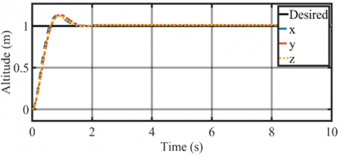
(a) Altitude responses
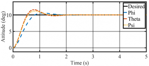
(b) Attitude responses
Figure 2. Nominal altitude & attitude responses
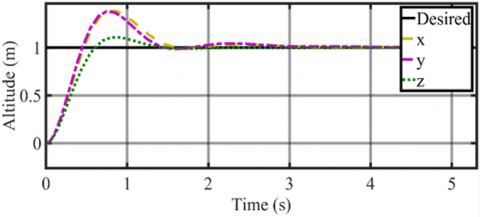
(a) Altitude responses
(b) Attitude responses
Figure 3. Uncertainty altitude & attitude responses
Table 2 shows the PID’s parameters gained from GA along with ITAE values. The parameters for the position controller were gained from applying (1 m) as a desired position while the those for attitude controller were gained by applying (10 deg) as a desired attitude. Figure 2 shows the altitude and attitude responses for the nominal system. The settling time for all the responses is less than 2 sec. Figure 3 shows the uncertainty response of the system after changing the mass from (2.3 kg) to (3 kg), and the arm length from (0.3 m) to (0.2 m).
The mathematical model of the tri-copter is implemented for simulation in MATLAB Simulink platform. Parameter values in Table 1 and Table 2 are used in the simulations. Table 2 also shows the ITAE values for the nominal system and the ITAE values of the uncertainty test. The result obtained using GE shows less ITAE than using a traditional tunning method with the PID compared with [4].
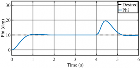
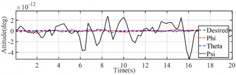
Figure 4 shows the response of the system to an impulse disturbance.
The system block diagram is shown in Figure 5. The validity and accuracy of the proposed controller are examined by applying two flight scenarios.
(a) disturbance on z axis
(b) disturbance on phi angle
Figure 4. System response to a disturbance
Figure 5. MATLAB Simulink block diagram
4.1 Circular flight
The scenario starts when the UAV initially at rest at (1,0,0) coordinates. It starts to fly to a one-meter height (1,0,1) in two seconds then it follows a circular path of one meter radius around the origin (0,0,0). The circular shape formula is:
$x=A_x \sin \left(\omega_x t\right)$ (45)
$y=A_y \cos \left(\omega_y t\right)$ (46)
where, $A_x=1, A_y=1, \omega_x=1\,\, \mathrm{rad} / \mathrm{sec}$, and $\omega_y=1 \,\,\mathrm{rad} / \mathrm{sec}$.
Figure 6 shows a circle path tracking flight. From the figure it can be noticed that there is a small deviation at the start of the circular path and this is due to the controller endeavour to catch the desired position. Once the actual UAV path coincided with the desired one, the response is stabilized, which is a proof of the designed controller accuracy.
Figure 6. Circle path scenario
Figure 7 shows the position and attitude responses during the flight. It can be seen that the system tracks the desired position well while keeping the attitude values at almost zeros. It means that the servo motors take the action to move the UAV to a desired position while keeping its body levelled.
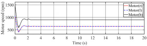
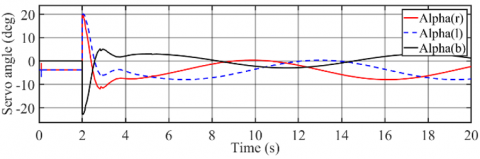
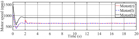
Figure 8 shows the servo angles and the motors speeds values during the circular path tracking. It is clear that the propeller speeds settle at a specific value while the servo motors updated continuously to help the UAV track the circular path.
(a) Altitude tracking
(b) Attitude tracking
Figure 7. Position and attitude tracking of the circular path
(a) Motors speeds
(b) Servos angles
Figure 8. UAV actuators responses during the circular flight scenario
4.2 Infinity shape flight
In order to test the system in more complicated situation, $\infty$ – shaped flight scenario is applied. The scenario starts at (0,0,0) coordinate. The UAV begins to fly to a one-meter height in two seconds. After that, it will start flying in an infinity shaped path. The path was created using the Eq. (43) and Eq. (44), where $A_x=1, A_y=0.5, \omega_x=1$, and $\omega_y=0.5$. Figure 9 shows the tracking of a flight path.
Figure 9. Infinity-shaped flight scenario
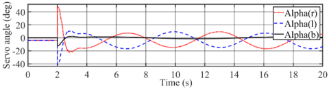
Figure 10 shows the position and the attitude tracking of the second scenario. It shows that the UAV tracks the desired altitude while keeping it attitude at zero. Thanks to the propellers thrust vectoring done by the servo motors to provide a horizontal force for the tri-rotor UAV movement. Figure 11 shows the servo angles and the motors speeds. Both the servos and the propellers did not exceed the pre-designed limits which is (-60, 60) degrees and (3600) rpm respectively.
(a) Altitude tracking
(b) Attitude tracking
Figure 10. Position and attitude tracking of the infinity path
(a) Motors speeds
(b) Servos angles
Figure 11. UAV actuators responses during the infinity flight scenario
To compare both scenarios the ITAE is calculated for the altitude during the flights and for both scenarios as shown in Table 3.
Table 3. Scenarios altitude ITAE values
|
Scenarios |
x ITAE |
y ITAE |
z ITAE |
|
Circle |
0.948 |
1.304 |
0.182 |
|
Infinity |
6.034 |
0.53 |
0.1899 |
The present work aims to provide a complete mathematical model along with a simple control scheme for the case of a tri-rotors UAV.
T shaped tri-copter is designed, and a complete non-linear mathematical model is formulated based on the Newton-Euler method and extracted using the system dynamic equations. Due to the strong coupling between rotational and translational output, the system is linearized using input-output feedback linearization method. The linear system is controlled using six PID controllers: Three for the position and the others for the attitude control. The PID controllers were tuned using GA as an optimization method to reach to the best performance in terms of the ITAE while maintaining the servo angles and rotors’ speeds in their design limits. Two flight scenarios are then performed to illustrate the overall system efficiency. These applied scenarios prove the controller ability to track different desired path with a very good performance. The frame of the UAV should be made using a strong light weighted materials such as carbon fiber for example. Brushless motors and (180 deg) servo should be used to construct the tiltable rotors along with gyroscopes, and a control unit. The battery should have high power capacity and it should be light weighted. Despite the all the results obtained so far including all the responses, disturbance test, uncertainty test, and scenarios the actual experimental model will define the validity of this model.
This work is completed due to Mechatronics Dep. support.
|
x |
x- axis, m |
|
y |
y- axis, m |
| z | z- axis, m |
| f | Force, N |
|
O |
Centre of mass |
|
a |
Length, m |
|
kf |
Force coefficient, $N . s^2$ |
|
kt |
Torque coefficient, $N.m.s { }^2$ |
|
m |
Mass, kg |
|
g |
Gravitational acceleration $\mathrm{m} / \mathrm{s}^2$ |
|
R |
Rotation matrix |
|
l |
UAV arm length |
|
Af |
Force constants matrix |
|
At |
Torque constants matrix |
|
Ax |
Constant |
|
Ay |
Constant |
|
I |
Body inertia, ${kg} . {m}^2$ |
|
v |
Velocity |
|
e |
Error |
|
Greek symbols |
|
|
a |
Servo angle, deg |
|
$\phi$ |
Roll angle, deg |
|
$\theta$ |
Pitch angle, deg |
|
$\psi$ |
Yaw angle, deg |
|
$\Psi$ |
Angular velocity rotation matrix |
|
$\tau$ |
Torque, $N.m$ |
|
$\lambda$ |
System output (altitude and attitude) |
|
$\sigma$ |
Attitude |
|
$\rho$ |
Altitude |
|
$\omega$ |
Angular velocity, r.p.m |
|
$\mu$ |
System input |
|
$\varsigma$ |
Compact system form |
|
$\beta$ |
Support symbol |
|
$\delta$ |
Support symbol |
|
$\Omega$ |
Total system output |
|
Subscripts |
|
|
r |
Right |
|
l |
Left |
|
b |
Back |
|
m |
Motor |
|
g |
Gravitational |
|
e |
Earth coordinates |
|
o |
Centre of mass coordinates |
|
v |
Vehicle |
|
p |
Proppeller |
|
d |
Drag |
|
f |
Force |
|
t |
Torque |
[1] Sabour, M.H., Jafary, P., Nematiyan, S. (2023). Applications and classifications of unmanned aerial vehicles: A literature review with focus on multi-rotors. The Aeronautical Journal, 127(1309): 466-490. https://doi.org/10.1017/aer.2022.75
[2] Cheng, D., Charles, A.C., Srigrarom, S., Hesse, H. (2019). Morphing concept for multirotor UAVs enabling stability augmentation and multiple-parcel delivery. AIAA Scitech 2019 Forum, No. 1063. https://doi.org/10.2514/6.2019-1063
[3] Sababha, B.H., Zu'bi, H.M.A., Rawashdeh, O.A. (2015). A rotor-tilt-free tricopter UAV: Design, modelling, and stability control. International Journal of Mechatronics and Automation, 5(2-3): 107-113. https://doi.org/10.1504/IJMA.2015.075956
[4] González, H., Arizmendi, C., Valencia, C., Valle, D., Bernal, B., Vera, A. (2021). Modelling and control system design for UAV tri-rotor. In AETA 2019-Recent Advances in Electrical Engineering and Related Sciences: Theory and Application, pp. 84-93. https://doi.org/10.1007/978-3-030-53021-1_9
[5] Houari, A., Bachir, I., Mohamed, D.K., Kara-Mohamed, M. (2020). PID vs LQR controller for tilt rotor airplane. International Journal of Electrical and Computer Engineering, 10(6): 6309-6318. https://doi.org/10.11591/ijece.v10i6.pp6309-6318
[6] Escareno, J., Sanchez, A., Garcia, O., Lozano, R. (2008). Triple tilting rotor mini-UAV: Modeling and embedded control of the attitude. In 2008 American Control Conference, Seattle, WA, USA, pp. 3476-3481. https://doi.org/10.1109/ACC.2008.4587031
[7] Salazar-Cruz, S., Lozano, R., Escareño, J. (2009). Stabilization and nonlinear control for a novel trirotor mini-aircraft. Control Engineering Practice, 17(8): 886-894. https://doi.org/10.1016/j.conengprac.2009.02.013.
[8] Salimi, S., Hashemzadeh, F., Khanmohamadi, S., Baradarannia, M. (2019). A new observer based Robust output feedback Controller on Coaxial Tri-copter. In 2019 27th Iranian Conference on Electrical Engineering (ICEE), Yazd, Iran, pp. 962-967. https://doi.org/10.1109/IranianCEE.2019.8786496
[9] Arroyo, A.D., Morais, A.S., Lima, G.V., Ribeiro, L. (2021). Modeling and simulation of a novel tilt-wing-coaxial-rotor tricopter. Simpósio Brasileiro de Automação Inteligente-SBAI, 1(1): 570-577. https://doi.org/10.20906/sbai.v1i1.2627
[10] Patel, S., Sarabakha, A., Kircali, D., Kayacan, E. (2020). An intelligent hybrid artificial neural network-based approach for control of aerial robots. Journal of Intelligent & Robotic Systems, 97(2): 387-398. https://doi.org/10.1007/s10846-019-01031-z
[11] Melo, A.G., Andrade, F.A., Guedes, I.P., Carvalho, G.F., Zachi, A.R., Pinto, M.F. (2022). Fuzzy gain-scheduling PID for UAV position and altitude controllers. Sensors, 22(6): 2173. https://doi.org/10.3390/S22062173
[12] Raheema, S.J., Saleh, M.H. (2021). An experimental research on design and development diversified controllers for tri-copter stability comparison. IOP Conference Series: Materials Science and Engineering, 1105(1): 012019. https://doi.org/10.1088/1757-899X/1105/1/012019
[13] Ahmed, N.M.A., Saleh, M.H. (2018). Tri-copter drone modeling with PID control tuned by PSO algorithm. International Journal of Computer Applications, 181(25): 46-52. https://doi.org/10.5120/IJCA2018918060
[14] Jalloh, M. S. (2021). Optimum design of unmanned aerial vehicles using structural optimization techniques. Doctoral dissertation, Bursa Uludag University, Turkey.
[15] Alkamachi, A., Ercelebi, E. (2017). Modelling and control of H-shaped racing quadcopter with tilting propellers. Facta Universitatis, Series: Mechanical Engineering, 15(2): 201-215. https://doi.org/10.22190/FUME170203005A
[16] Penkov, I., Aleksandrov, D. (2017). Efficiency optimization of mini unmanned multicopter. International Review of Aerospace Engineering, 10(5): 267-276. https://doi.org/10.15866/irease.v10i5.12132
[17] Martinez, R.R., Paul, H., Shimonomura, K. (2023). Aerial torsional work utilizing a multirotor UAV with add-on thrust vectoring device. Drones, 7(9): 551. https://doi.org/10.3390/drones7090551
[18] Anuar, K., Fatra, W., Akbar, M. (2020). Tricopter vehicle frame structure design integrated as platform of fixed wing Atha Mapper 2150. Journal of Ocean, Mechanical and Aerospace, 64(2): 68-72.
[19] D'Amato, E., Di Francesco, G., Notaro, I., Tartaglione, G., Mattei, M. (2015). Nonlinear dynamic inversion and neural networks for a tilt tri-rotor UAV. IFAC-PapersOnLine, 48(9): 162-167. https://doi.org/10.1016/j.ifacol.2015.08.077
[20] Innocenti, M. (1999). Helicopter flight dynamics: The theory and application of flying qualities and simulation modeling. Journal of Guidance, Control, and Dynamics, 22(2): 383-384. https://doi.org/10.2514/2.4396
[21] Rao, V.G., Bernstein, D.S. (2001). Naive control of the double integrator. IEEE Control Systems Magazine, 21(5): 86-97. https://doi.org/10.1109/37.954521
[22] Alkamachi, A., Erçelebi, E. (2017). Modelling and genetic algorithm based-PID control of H-shaped racing quadcopter. Arabian Journal for Science and Engineering, 42: 2777-2786. https://doi.org/10.1007/S13369-017-2433-2
[23] Astrom K.J. Hagglund, T. (1995). PID Controllers: Theory, Design, and Tuning. ISA - The Instrumentation, Systems and Automation Society.
[24] Sumida, B.H., Houston, A.I., McNamara, J.M., Hamilton, W.D. (1990). Genetic algorithms and evolution. Journal of Theoretical Biology, 147(1): 59-84. https://doi.org/10.1016/S0022-5193(05)80252-8