Hawraa A. Al-Ta'I*![]() | Riyadh Toman Thahab
| Riyadh Toman Thahab![]()
© 2024 The authors. This article is published by IIETA and is licensed under the CC BY 4.0 license (http://creativecommons.org/licenses/by/4.0/).
OPEN ACCESS
Distribution networks are employing more power electronics devices to achieve several desired objectives. Soft Open Points (SOP) are one of these devices that tend to be implemented in points that are normally open in a radial structured system. In this work control of power converters from which SOPs are constructed is first investigated in the atmosphere of a test distribution system. The primary step in setting up the controls is to obtain the reference real and reactive power settings per converter required to minimize the cost functions set out by the distribution system operator. Through an adaptive Particle Swarm Optimization (PSO) the former mentioned power settings were determined based on a desired cost function to be minimized. In this work, the control settings where first implemented using PI controllers for each converter. An approach is proposed in which a combination of two different control methods is employed. This hybrid approach is based on controlling one of the converters in PI synchronous reference frame environment while the other converter is based on a hysteresis current controller which corresponds to the power references obtained for that specific converter. The proposed method is implemented on the IEEE33 bus distribution system and simulated in MATLAB/SIMULINK. Results show the effectiveness of the proposed hybrid approach in reducing the number of required PI controllers and eventually the effort of parameter tuning. Furthermore, the hybrid approach shows considerable reduction in, overshoots of actual bus power signals and tracking errors. These improvements are reflected directly in the bus voltage profiles at the points of SOP connections and other buses of distant radials. Moreover, the aforementioned features of the proposed approach directly affect the reliability of power delivered to consumers’ feeders at the SOP connection points and others within its vicinity.
soft open points, particle swarm optimization, PI controller, hybrid approach
Distribution networks are considered the terminal zone where generated electrical power finally reach consumers. Characteristics of these distribution networks directly impact consumers’ appliances. Conventionally, networks are design to be of radial formation with an alternative ring topology in some applications. The former has the characteristics of been easy to operate, control and protect whereas the latter need expensive protection strategies. Reliability wise, ring formation has proven to be more reliable since an interconnection exists between adjacent radials, a benefit that is absent in a pure radial topology. Modern distribution networks are becoming considerably active due to the use of energy sources which are scattered in a vicinity of network. Several countries wish to utilize distributed energy resources, resulting in a more active distribution network [1, 2]. However, increasing the number of activeness level, in a distribution network, may result in an unbalanced power flow across radial feeders, owing to various loading scenarios. As a result, there are significant power losses, increased peak currents, and undesired voltage excursions [3]. Distribution networks are increasingly being converted from their original radial form to a largely closed loop topology [4, 5] as an approach to solve the aforementioned problems.
The load can be balanced across feeders in a closed loop or ring arrangement as opposed to a radial one, optimizing voltage profiles and enhancing power supply dependability [5]. More difficult and expensive protection methods are needed for a closed loop network design [5, 6].
In a radial distribution network there exist many points that are normally open points (NOPs) which can be devoted to facilitate a compromise between a pure radial structure and an expensive ring [4]. It has been proposed that Soft Open Points (SOPs), constructed from two power converter devices, replace NOPs in a distribution network, which can combine the benefits of radial and loop (mesh) operated networks while avoiding the disadvantages of each [6]. The advantages of SOPs for the operation of distribution networks have been highlighted in prior studies [6-8], with the majority of these studies focusing on standard network operation restrictions. SOPs are two converters operated in a back- back fashion with a mid-DC link [9]. Back-back converters find numerous applications that include, integration of wind power systems [10], high voltage DC transmission and induction machine drives [11]. In applications where back-back converters are used as power flow controllers, which is equivalent to the operation of an SOP, control can be applied that includes controlling one of the converters to provide a constant dc link voltage while the other is operated to control real and reactive power flow [12, 13]. In study [14], an external loop is designed to provide reference quantities which are tracked by an internal loop designed based on state feedback control, where the back-back converters are used to interface a micro grid into an AC network. Zhang et al. [15] proposed a control scheme for back- back converters based model predictive control for the grid side converter. The DC link voltage is implicitly controlled through the model predictive system thereby eliminating the PI controller for the DC link capacitor. Authors report that although the proposed non-PI system performs well in normal conditions, yet robustness is higher in case of discrepancy of system parameters for the PI based controls. A multivariable approach to control back-back converters is presented in study [16], here variables to be controlled are first separated as low and high frequency components and a controller is designed to perform reference tracking and disturbance rejection.
Hysteresis control is another approach that is widely used to control converters due to its simplicity and the straight forward implementation [17, 18]. Usually, hysteresis is a current controller that is designed in the abc stationary frame [17]. The use of a combined PI and hysteresis controller is presented in studies [18, 19] for only one converter which interfaces DC power into an AC system. The high switching activity of a hysteresis controller, which is considered a drawback, can be reduced through maintaining the same polarity of phase voltage for one third of the total one cycle time [18].
Present work on SOPs mainly deals with two aspects; the first is quantization of the benefits in terms of reduced real power losses, improvement in voltage profile and an enhanced balancing of feeders [20]. The second is investigation and enhancement of the adopted optimization method [20]. Control of back- back converters in SOP applications has been mentioned in study [21], where response of conventional PI controllers are illustrated due to a step change in both active and reactive powers and its effect on maintaining a constant DC link voltage. The main challenges in integrating SOPs into distribution systems are; optimizing the operating points of the device which implies employing an optimization algorithm that minimizes a set of cost functions set out by the distribution system operator. The second challenge is implementing those optimum points via an accurate and reliable control system.
In this work the main emphases is related to the control system of an SOP device, which requires an important preliminary step of obtaining the reference settings. A proposed control method is presented that is based on a hybrid approach, where each converter of the SOP has a control method that differs from the other. To the best of our knowledge, a gap exists in existing literature, between determination of the optimal operating points of an SOP, which are considered the control reference settings in this work, and utilizing them in the control system. Therefore, the present work aims to bridge this gap by employing the operating points found through optimization techniques in the design of the control system that manages SOP operation. To assess the control objectively, the proposed hybrid method is tested on a standard distribution network with multi radials and buses that supply a variety of load values.
The rest of this paper is organized as follows: section 2 presents description and mathematical model of SOP, section 3 presents references generation for control system of SOP Converters, section 4 displays Proposed Hybrid Control Approach for SOP Converters and section 5 shows simulation and results.
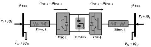
Power electronics converters, in back-back formation, can be used to replace open points, usually situated on feeders ends [6]. With this formation, a link is provided between two radials of a network which is utilized to export or import power according to the status of the corresponding radial. Hence, an SOP is usually modelled as a flow of real/reactive power between buses at the end of radials that are considered open points [6]. Reference to Figure 1 (a), buses i & j are normally open points, an SOP device is connected at these end buses. The amount of apparent power injected or supplied at either end is defined as, $P_{V S C-i}+j Q_{V S C-i}$ for converter i and $P_{V S C-j}+j Q_{V S C-j}$ for converter j. The standard practice in power analysis of distribution networks is to calculate the power flow injected into a bus depending on the flow from the bus before it [20]. Hence, real and reactive power at bus i prior to the connection of an SOP is,
$\begin{aligned} P_i & =P_{i-1}-P_{L i}-P_{ {Loss }(i, i-1)} \\ Q_i & =Q_{i-1}-Q_{L i}-Q_{ {Loss }(i, i-1)}\end{aligned}$ (1)
And for converter j,
$\begin{aligned} P_j & =P_{j-1}-P_{L j}-P_{ {Loss }(j, j-1)} \\ Q_j & =Q_{j-1}-Q_{L j}-Q_{ {Loss }(j, j-1)}\end{aligned}$ (2)
where, $P_{i(j)-1} / Q_{i(j)-1}$, $P_{\text {Li(j) }} / Q_{\text {Li(j) }}$ and $P_{\text {Loss }(i(j), i(j)-1)} /$$Q_{\text {Loss }(i(j), i(j)-1)}$ are the real/reactive; power flow of the bus preceding the $i^{t h}\left(j^{t h}\right)$ bus, load values at the $i^{\text {th }}\left(j^{\text {th }}\right)$ bus and losses of resistive /reactive line parameters connecting the $i^{\text {th }}\left(j^{\text {th }}\right)$ bus to the preceding bus $i^{\text {th }}\left(j^{t h}\right)-1$, respectively.
In the presence of the SOP, a schematic of which is shown in Figure 1 (b), a new real/reactive power flow which corresponds to that of the respective converter apparent power values are incorporated into Eq. (1) and Eq. (2). Assuming that the converter and relevant filter has no real losses [22], Eq. (1) and Eq. (2) become,
$\begin{aligned} P_i+P_{V S C-i} & =P_{i-1}-P_{L i}-P_{\text {Loss }(i, i-1)} \\ Q_i+Q_{V S C-i} & =Q_{i-1}-Q_{L i}-Q_{\text {Loss }(i, i-1)}\end{aligned}$ (3)
For bus i. While for bus j,
$\begin{aligned} P_j+P_{V S C-j} & =P_{j-1}-P_{L j}-P_{L o s s(j, j-1)} \\ Q_j+Q_{V S C-j} & =Q_{j-1}-Q_{L j}-Q_{L o s s(j, j-1)}\end{aligned}$ (4)
Usually the sign of the real and reactive power of each VSC determines whether the power flows outwards or inwards with respect to the bus. Eq. (3) and Eq. (4) provides a general inclusion of the SOP system powers at the two buses of connection. To preserve a real power equilibrium, the algebraic sum of power for converters must add to zero [22]. Hence,
$P_{V S C-i}+P_{V S C-j}=0$ (5)
(a)
(b)
Figure 1. (a) An SOP connection between two open ended points for part of a distribution network. (b) main circut of back to back based SOP based on a two level topology [21]
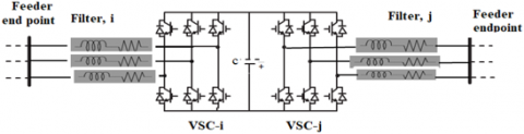
Figure 2. PI based compact control block diagram of two back- back converters for an SOP between the $i^{\text {th }}$ and $j^{t h}$ bus
Or,
$P_{V S C-i}=-P_{V S C-i}$ (6)
Clearly from Eq. (6), one of the buses must have real power injected whereas the other supplies this power. The reactive power for each VSC of an SOP can be either determined based on fulfilling certain voltage requirements [23] or from an optimization method which defines the optimal operating points of the entire SOP system. It is clearly noted that an SOP provide a link between two points on a radial system that would otherwise be normally open. Therefore, with this power electronics system, if a case of surplus real power exist on one radial, it can be used to curve a shortage on the other. In the meantime reactive power import/export can be used to remedy a decrease or an increase of voltage profiles in the targeted radials of SOP connection.
Usually control of the back-back converter configuration is application orientated. A general requirement of the controls is that the real power flow between the converters must be balanced [22]. One of the converters for example, $V S C 1$,must be controlled to maintain a constant voltage profile at the DC link terminals [21]. The former is achieved if and only if the DC link capacitor does not absorb nor supply any power to alter the real power balance. On the other hand, $V S C 1$, can also be used to control reactive power of the AC terminals when the back-back system is used to interface two AC system with a power factor less that unity.
The second converter, VSC2, can be handled to control real and reactive power at the AC system to which its connected to [21]. Usually the control of the apparent power is transferred to be a current control objective. If the control is implemented in the stationary αβ frame, the controls are reduced to regulating the components of the AC system [23, 24], whereas, in the rotating $d q$ frame the process involves regulation of $i_d$ & $i_q$ components [24]. Figure 2, shows the conventional control for the two $V S C_i$ & $V S C_j$ in the $d q$ frame. The latter system has two additional PI controllers that compares reference/required real and reactive powers, $P_{\text {ref }-j}$/$P_{v s c-j}$ & $Q_{r e f-i / j} / Q_{v s c-i / j}$, to produce the required control signal [13]. For, $V S C_i$, the control loop are usually nested, which means an external loop provides a reference current setting for an internal loop which provides current regulation for $i_d$ [13, 21]. However, the $i_q$ component is regulated in separate current loop. Conventionally all regulating loops have PI controllers that provides tracking of the variables to be controlled. The final stage of this conventional control is generating the dq voltage modulating signals, V_{\text {dmod } i / j} \text { and } V_{\text {qmod } i / j} \text { for the } i^{t h} \text { and } j^{t h} as shown in Figure 2. Hence, these current signals are DC by nature since they rotate at exactly the same speed as the abc frame, enabling the use of conventional PI controllers. The speed of rotation is usually determined by a phase locked loop (PLL) [21].
A major target of control systems is that a controlled variable needs to track a reference setting with minimum possible error. An integral part of this work is determination of the various references required for the operation of the controls. For SOPs these reference settings are determined from an optimization process. In this work, an optimization algorithm is employed that minimizes one, from a set, of defined cost functions. The algorithm is based on the particle swarm optimization (PSO) method [25]. Usually, the cost functions that need to be minimized involve; real power losses in the distribution system, voltage profile deviations and feeder load balancing which are defined as [20].
$\begin{array}{r}\text { Obj1 }=\sum_{k=1}^{N branch}\left(P^k-P^{k+1}\right) \\ \text { Obj2 }=\sum_{n=1}^{N b u}\left|\left(V_n-V_{n_{-} r e f}\right)\right| \\ \text { Obj3 }=\sum_{k=1}^{\text {Nbranch }} \frac{\mathrm{I}_{\text {flow_k }}}{\mathrm{I}_{\text {rated_k }}}\end{array}$ (7)
where, $P^k$ & $P^{k+1}$ are the active power flow for bus $k$ and $k$ +1 respectively, $V_n$ is voltage for $n^{t h}$ bus and $V_{n \_r e f}$ is the reference voltage, which is considered as 1 P.U., based on the nominal voltage of the distribution system. $\mathrm{I}_{\text {flow } k}$ is the current flow in the $k^{t h}$ branch connecting bus $k$ to the next bus, which is, $k+1$, $\mathrm{I}_{\text {rated } k}$ is the rated current of branch $k$. Nbranch is the total number of branches and Nbus is the number of bus-bars.
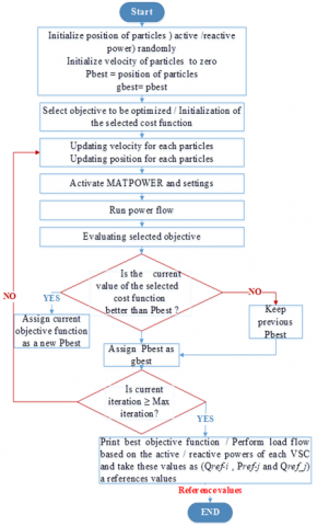
For the present work, the emphases is based on finding the optimal operating points of the SOP, that include:$P_{r e f-i}$, $Q_{\text {ref-i }}$, $P_{r e f-j}$, and $Q_{r e f-j}$. Three of these powers are directly employed in the respective control system of a converter from which the SOP is composed. The proposed optimization algorithm is based on a single objective PSO which minimizes one cost function [26]. In this work, the PSO is modified to be an adaptive approach that minimizes a defined cost function. The suggested approach gives the flexibility to distribution system operators to utilize the SOP device to accommodate minimization of a selected cost function based on the time status of the network. The adaptive algorithm can be summarized in the following points:
Figure 3 shows the algorithm flow chart and algorithm table shows a pseudo code of PSO. In this work the load flow is implemented using MATPOWER [27] and is embedded with the PSO algorithm.
Figure 3. Flow chart of control of SOP (using particle swarm optimization algorithm)
|
Algorithm: Pseudo Code of PSO |
|
1: Set SOP location for: set i & j |
|
2: Set MVA rating for each SOP converter |
|
3: Determine cost function to be minimized, Obj1, Obj2 or Obj3 |
|
4: For k=1: number of populations |
|
5: Initialize population members for SOP, $S_{\text {intial }}$ = $\left[\begin{array}{lll}Q_{\text {ref-i }} & Q_{\text {ref-j }} & P_{\text {ref-j }}\end{array}\right]^{\text {intial }}$ |
|
6: Initialize velocity to zero |
|
9: Initialize cost function |
|
10: Personal best solution = random solution |
|
11: Best cost function= cost function |
|
12: End |
|
13: For 1: Maximum number of iterations |
|
14: For 1: Number of population |
|
15: Update velocity |
|
16: Update position |
|
17: If updated position satisfies the constrains, $S_{r e f-i} \leq$ $\sqrt{P_{r e f-i}{ }^2+Q_{r e f-i}{ }^2}$ & $S_{r e f-j} \leq \sqrt{P_{r e f-j}^2+Q_{r e f-j}^2}$ |
|
18: Run MATPOWER and perform load flow |
|
19: Calculate the value of the selected cost function with the present solution |
|
20: If the current solution is better than the former, update Pbest and gbest |
|
21: End if maximum number of iterations is reached |
|
22: Store final solution and corresponding cost function, $\left[\begin{array}{lll}Q_{r e f-i} & Q_{r e f-j} & P_{r e f-j}\end{array}\right]^{\text {final }}$ |
3.1 Dynamic analysis of voltage controller based on the generated references
In this section dynamic analysis is presented for the voltage control of one of the SOP converters. The aim is to study the response of control system corresponding to the value of power that this converter may supply or absorb depending on the results of the optimization process of an SOP. To determine the open loop transfer function. Refer with: Figure 2, it is assumed that $V S C_i$ controls the DC voltage of the DC-link capacitor. Hence, the capacitor current is expressed as,
$C \frac{d V_{D C}}{d t}=i_c$ (8)
Multiplying Eq. (8) by $V_{D C}$ will result in an expression of rate of change of power at the capacitor terminals, which is equal to the difference in powers at both ends of the capacitor. For the SOP system, this is expressed as,
$\frac{C}{2} \frac{d V_{D C}^2}{d t}=P_{v s c-j}-P_{v s c-i}$ (9)
Using the space phasor representation [28], the voltage balance equation at the terminals of $V S C_i$ is written as,
$L_i \frac{d \vec{\imath}}{d t}=-R_i \vec{\imath}+\vec{V}_{v s c i}-\vec{V}_i$ (10)
where, $\vec{l}$, $L_i$, $R_i$, $\vec{V}_{v s c i}$ and $\vec{V}_i$ are the current phasor, inductance, resistance, terminal converter voltage and bus bar voltage of the $V S C i$ of the SOP device respectively. Here, since the dq synchronous frame is used, the respective space phasors are defined as [28],
$\begin{gathered}\vec{\imath}=i_d+j i_q \\ \vec{V}_{v s c i}=V_{v s c d}+j V_{v s c q} \\ \vec{V}_i=V_{i d}+j V_{i d}\end{gathered}$ (11)
If Eq. (10) is multiplied by $(3 / 2) \vec{l}^*$, this equation is transformed to a power balance form,
$\frac{3}{2} L_i \frac{d \vec{l}}{d t} \times \vec{\imath}^*=-R_i\left(\frac{3}{2} \vec{\imath} \times \vec{l}^*\right)+\vec{V}_{v s c i}\left(\frac{3}{2} \vec{l}^*\right)-\vec{V}_i\left(\frac{3}{2} \vec{l}^*\right)$ (12)
Which is simplified to,
$\begin{gathered}\frac{3}{2} L_i \frac{d \vec{l}}{d t} \times \vec{\imath}^*=-\frac{3}{2} R_i \times i^2+\left(P_{v s c-i}+j Q_{v s c-i}\right)- \left(P_i+j Q_i\right)\end{gathered}$ (13)
The term $\frac{d \vec{\imath}}{d t} \times \vec{\imath}^*$, can be further expanded as,
$\frac{3}{2} L_i \frac{d \vec{l}}{d t} \times \vec{\imath}^*=\frac{3}{2} L_i \frac{d}{d t}\left(i_d+j i_q\right) \times\left(i_d-j i_q\right)$ (14)
Which is further simplified to,
$\frac{3}{2} L_i \frac{d \vec{\imath}}{d t} \times \vec{l}^*=\frac{3}{2} L_i\left[\left(i_d \frac{d i_d}{d t}+i_q \frac{d i_q}{d t}\right)+j\left(i_d \frac{d i_q}{d t}-i_q \frac{d i_d}{d t}\right)\right]$ (15)
The real part of Eq. (15) can be written as,
$\left(i_d \frac{d i_d}{d t}+i_q \frac{d i_q}{d t}\right)=\frac{1}{2} \frac{d}{d t}\left(i_d^2+i_q^2\right)=\frac{1}{2} \frac{d i^2}{d t}$ (16)
The power term $\left(P_{v s c-i}+j Q_{v s c-i}\right)$ in Eq. (13) can be written with the aid of Eq. (14-16) as,
$\begin{aligned} P_{v s c-i}+j Q_{v s c-i}= & \frac{3}{4} L_i \frac{d i^2}{d t}+j \frac{3}{2} L_i\left(i_d \frac{d i_q}{d t}-i_q \frac{d i_d}{d t}\right) \\ & +R_i \times i^2+\left(P_i+j Q_i\right)\end{aligned}$ (17)
Furthermore, the current at the $i^{\text {th }}$ bus bar of the system is,
$i^2=\frac{4}{9} \times \frac{P_i{ }^2+Q_i{ }^2}{V_i^2}$ (18)
Hence Eq. (18) become,
$\begin{aligned} & P_{v s c-i}+j Q_{v s c-i}=\frac{3 L_i}{4 v_i^2} \times \frac{4}{9}\left(2 P_i \frac{d P_i}{d t}+2 Q_i \frac{d Q_i}{d t}\right)+ \\ & P_i+\frac{4}{9} R_i \times \frac{P_i{ }^2+Q_i^2}{V_i^2}+j\left[\frac{3}{2} L_i\left(i_d \frac{d i_q}{d t}-i_q \frac{d i_d}{d t}\right)+Q_i\right]\end{aligned}$ (19)
Since Eq. (9) considers real power balance, the real part of Eq. (19) is considered. Therefore, Eq. (9) reduces to,
$\begin{gathered}\frac{d V_{D C}^2}{d t}=\frac{2}{c} P_{v s c-j}-\frac{2}{c}\left[P_i+\frac{2 L_i}{3 v_i^2}\left(P_i \frac{d P_i}{d t}+Q_i \frac{d Q_i}{d t}\right)+\right. \left.\frac{4}{9} R_i \times \frac{P_i^2+Q_i^2}{V_i^2}\right]\end{gathered}$ (20)
Eq. (20) can be linearized using the small signal perturb method around a defined steady state point [28]. The deviation in DC link voltage to deviation in converter injected power transfer function can be found by neglecting dynamics of bus voltage and assuming a zero rate of change in reactive power and assuming the filter resistance is small enough to be neglected [28]. Hence,
$\frac{d \widetilde{V_{D C}^2}}{d t}=-\frac{2}{C}\left\lceil\widetilde{P}_i+\frac{2 L_i P_{i o}}{3 V_i^2} \times \frac{d \widetilde{P}_l}{d t}\right\rceil$ (21)
In the S-domain the transfer function is defined as,
$\frac{\widetilde{V_{D C}^2}}{\widetilde{P_l}}=-\left(\frac{2}{C}\right) \frac{\left(2 L_i P_{i o} / 3 V_i^2\right) S+1}{S}$ (22)
From Eq. (22), the voltage controller transfer function is obtained. Here, the response is evaluated based on how well a deviation in the DC voltage can be nullified [28]. To find the frequency response of the controller for the SOP converter that control the DC voltage, the open loop transfer.
$L(S)=G_{P i-v}(s) \times G_{\text {in-loop }}(s) \times G_{\widetilde{{V_{D C}^2} / \widetilde{P}_l}}(s)$ (23)
$G_{V_{D C}^{\widetilde{2}} / \widetilde{P}_l}(s)$ is the transfer function defined by Eq. (22). In this analysis all of these transfer functions parameters will be expressed in per unit system. To obtain the frequency of the voltage controller for the $i^{\text {th }}$ converter of the SOP system, the steady state power, must be known. If the switching losses are also neglected then this power, $P_{i o}$, is approximately equal to the real power of the converter, $P_{v s c-i}$. Based on the controller tracking performance, then,
$P_{r e f-i} \approx P_{v s c-i}$ (24)
The power, Pref-i, is found by applying the PSO method explained in section 3 of this paper. This optimization method was applied on the IEEE 33 bus system [29], at two tie switch positions, that is the 25-29 and 8-21 locations. In these two positions, an SOP is connected one at time. Since the optimization algorithm requires determination of a cost function, only ohmic losses are considered in this work which is objective 1 of Eq. (7). Table 1 shows the results of the optimization in terms of real/reactive powers that represent the optimal operating points according to the selected cost function.
Table 1. Optimum real/reactive powers for converters of the SOP system based on PSO
|
Location of SOP |
Cost Function Targeted (Losses in Kw) |
$Q_{ {ref- } i}$ MVAR |
$Q_{ {ref- }} 1$ MW |
$Q_{ {ref-1 }}$ MVAR |
$P_{r e f-1} I$ MW |
|
25-29 |
131.583 |
- 0.474 |
0.611 |
-1.237 |
-0.611 |
|
8-21 |
123.356 |
- 1.119 |
-1.053 |
- 0.184 |
1.053 |
Based on the above real power point of $V S C_i$, the transfer function, $G_{P i-v}(s)$ can be defined. For simplicity the term, $\left(2 L_i P_{i o} / 3 V_i^2\right)$, can be expressed in per unit system, in which the base apparent power is $3 \mathrm{MVA}$ at a nominal system voltage of $12.66 \mathrm{KV}$. Moreover, the PI voltage controller parameters are tuned using the modulus optimum method [24].
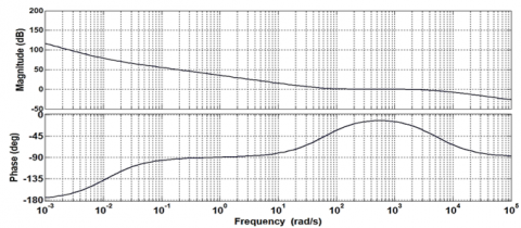
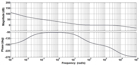
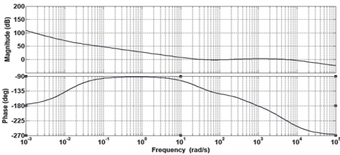
Reference to Figure 4 shows the Bode plots for the transfer function of $V S C_i$ of the SOP device at location 25-29 of the distribution system. Here, a current time constant of $2 \times 10^{-4} S$ is assumed for, $G_{\text {in-loop }}(s)$. The voltage controller is assumed to be 50 times slower than the current controller, hence the gain is set such that the angular cross over frequency is 200 rad/sec. Clearly, the system possess, at this location, close loop stability since the phase is around, $-10.4^{\circ}$. For the location $8-21$, where the optimization reveals that the $V S C_i$ converter has a negative input real power, or supplies positive power through the DC link to the $V S C_j$ converter. Figure 5 , shows the frequency response for the controls of this converter. Since the value of inductance and capacitance are assumed to be the same, the same PI parameters are employed. For easy comparison, the same cross over frequency is assumed for 8-21 as that of 25-29 location, the phase is reported to be approximately $-180^{\circ}$ which can be considered just about unstable. This situation can be remedied by introducing a lead compensator [28]. If a lead compensator is added to the open loop transfer function defined by Eq. (23), the close loop transfer function has a phase margin of $30^{\circ}$ at the 200 rad/sec, cross over frequency. Figure 6 shows the frequency response for the 8-21 location, where the phase is now $-150^{\circ}$ at the frequency of 200 rad/sec.
The dynamic analysis presented here confirms that the controller design is dictated by the position of the SOP device within the distribution system. Once, the location is determined then the controller requirements will depend on the power flow direction of one of the converter which is employed to provide a constant DC link voltage. Moreover, this power flow, in value and sign, is obtained from the optimization process. Therefore, the optimization process plays a pivotal role in the controller design and response.
Figure 4. Bode plots for VSCi converter of the SOP system at location 25-29
Figure 5. Bode plots for VSCi converter of the SOP system at location 8-21 with no lead compensator
Figure 6. Bode plots for VSCi converter of the SOP system at location 8-21 with a lead compensator at 30° phase margin
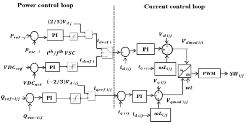
Conventional control of back-back converters which require one PI voltage controller and four PIs for current control resulting in a number of parameters to be tuned. If power integrators are employed that produce the error, which is the difference between reference and actual components of apparent power for each converter [13], then about eight PI controllers are required. This will further increase the number of parameters to be tuned. In this work a control method is suggested that eliminates the PI controllers for one of the converters which results in a significant reduction in the number of those controllers. It is proposed that one of the converters is controlled via the hysteresis current controller method [19] which utilizes the real/reactive powers of the SOP system obtained from the optimization technique. Furthermore, based on simple calculations, the reference current settings are obtained which are converted to stationary abc frame. The hysteresis controller simply compares between those references and actual currents to decide on the switching status of the controller based on the predefined hysteresis band [19]. For the converter, $V S C_j$, which controls the optimized real/reactive power, the optimum operating point can be expressed in terms of voltage and current as,
$P_{r e f-j}=\frac{3}{2}\left(V_{d j} \times I_{d r e f j}+V_{q j} \times I_{q r e f j}\right)$ (25)
And for reactive power
$Q_{r e f-j}=\frac{3}{2}\left(-V_{d j} \times I_{q r e f j}+V_{q j} \times I_{d r e f j}\right)$ (26)
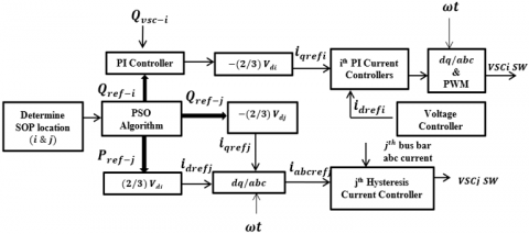
If the dq synchronous reference frame is rotated at the same speed of the AC grid, which is detected by a phase locked loop [24], then $V_{q j}$ is nullified [24], and the real/reactive power is function of the current $I_{\text {dref } j} \& I_{\text {aref } j}$. Those currents are the reference settings in dq frame. Figure 7 , below shows a block diagram of the proposed hybrid control method for the SOP device connected between bus $i \& j$ of a distribution power system.
Figure 7. Block diagram of the proposed hybrid control system of an SOP device connected between ith & jth bus
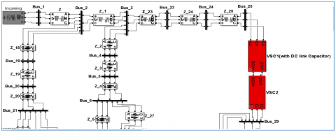
In this part simulations are carried out to verify the feasibility of the control approach suggested in this work. As a first step, the conventional PI controllers are simulated on the IEEE 33 system, where total active and reactive load demands are, 3715 KW and 2300 KVAR [29] respectively. Simulations are carried out in MATLAB/SIMULINK. All parameters used are shown in Table 2. First, the SOP location is determined, in this study the same two locations are considered; 25-29 and 8-21 as mentioned in section 3.1 of this paper. Although the PSO algorithm is designed to optimize the distribution system cost functions defined by Eq. (7), however in this work we will consider only minimization of real power losses only. Figure 8, below shows part of the IEEE 33 system with the SOP (and embedded controller) connected between bus 25 and 29.
Table 2. Simulation parameters
|
Parameter |
Value |
|
Rated VSC apparent power /Base MVA |
3 MVA |
|
Nominal grid voltage/Base voltage |
12.66 KV vrms |
|
Number of populations for PSO |
40 |
|
Number of particles |
4 |
|
Maximum number of iterations |
60 |
|
Personal Acceleration coefficient (C1) for PSO, global Acceleration coefficient(C2) for PSO |
1, 2 [30] |
|
Two random variables for PSO r1, r2 |
(0-1), (0-1) [30] |
|
DC-link voltage |
30 KV |
|
Line frequency |
50Hz |
|
Switching frequency |
1300 Hz |
|
RL filter of each converter |
R = 0.22 Ω, L = 20 mH |
|
DC-link capacitance |
C = 200 µF |
Figure 8. Part of IEEE 33 system with SOP connected between buses 25 and 29
5.1 Simulation results of conventional PI controller
As a first step, PI controllers were used to track the reference DC voltage and the optimized values of real/reactive that were obtained from the PSO algorithm.
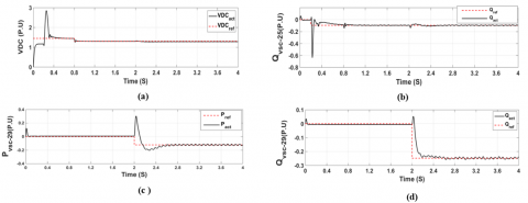
The sequence of events are as follows, first, at $t=0\,\, \mathrm{sec}$, both converters are inoperative and the capacitor is charged to a $1.5\,\, \underline{\mathrm{P.U}}$ of voltage, then at $t=0.2\,\, \mathrm{sec}$, converter at bus 25 is fired, an over shoot of more than 2.5 P.U is observed before the voltage settles to its steady state value at, $t=0.4\,\, \mathrm{sec}$. Furthermore, a change in the step value of the reference voltage is initiated at, $t=0.8 \mathrm{sec}$, where the controller is able to track the new reference setting. Tracking performance of the DC voltage controller is depicted in Figure 9 (a). The controller for this converter also tracks the optimal reactive power, $Q_{v s c-25}$, the tracking performance is shown in Figure 9 (b). An overshoot occurs before the controller tracks the reactive power, it is interesting to note that the response of the reactive power is momentarily effected by the change in the DC reference voltage which was initiated at $0.8 \mathrm{sec}$. This is attributed to dynamics overlap of the converter system.
Converter 2 , which is connected at bus 29 , is triggered at $t=2\, \mathrm{sec}$. The controller tracks the per unit, step unit modulated, reference setting which is obtained from the PSO algorithm, $P_{\text {ref-29}}$. Tracking performance is shown in Figure 9 (c). Prior to the to the $2\, \mathrm{sec}$ simulation time, the controller is idle and the actual real power is almost zero. After a delay, controller track the $P_{r e f-29}$ reference, however some oscillations are observed in the actual measured power, $P_{v s c-29}$. Finally, the reactive power of this converter, $Q_{v s c-29}$, tracking performance is depicted in Figure 9 (d), where also an amount of oscillations is observed in the actual reactive power measured at bus 29 .
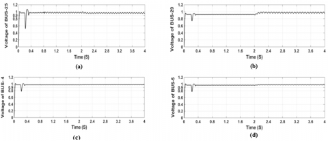
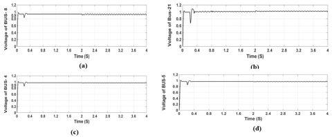
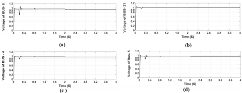
The majority of converter control systems is evaluated based on the tracking performance of the controller employed. However, in SOP applications, the controller assessment must consider the effects on the respective bus voltage profile where the SOP is connected. Also, connection effects of the SOP is evaluated for buses of nearby radials of the distribution systems. Figure 10 (a) and (b) show the per unit voltage suffers a momentarily voltage dip before restoring to steady state value. On the other hand, voltage profiles at bus $25 \& 29$ respectively. Here, at bus 25 , it is seen that voltage suffers a momentarily voltage dip before restoring to steady state value. On the other hand, voltage profile at bus 29 shows a less pronounced voltage dip when converter 1 is triggered at, $t=0.2\,\, \mathrm{sec}$ before restoring back to nominal value. As converter 2 is triggered at $t=2\,\, \mathrm{sec}$, voltage profile is increased since the sign of $Q_{r e f-29}$ is negative which means the bus injects reactive power. Both voltage profiles show oscillations due to the switching action of the converters. Finally, voltage profiles at a two distant buses are shown in Figure 10 (c) and (d). These profiles show less effect of the SOP actions connected at location 25-29. As seen in Figure 10 (c) and (d), voltage profile suffers less dips in voltage due to SOP converter switching.
Figure 9. Tracking performance of conventional PI based controller for an SOP at location (25-29): (a) dc side voltage, (b) reactive power response of VSC 25, (c) active power response of VSC 29 and (d) reactive power of VSC 29
Figure 10. Voltage profiles of the IEEE 33 system for PI based controllers of SOP at: (a) bus 25, (b) bus 29, (c) bus 4 and (d) bus 5
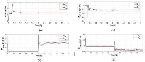
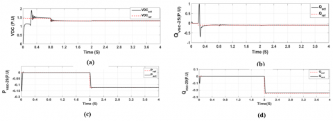
Figure 11. Tracking performance of conventional PI based controller for an SOP at location (8-21): (a) dc side voltage, (b) reactive power response of VSC 8, (c) active power response of VSC 21 and (d) reactive power response of VSC 21
Figure 12. Voltage response of the IEEE 33 system for PI based controllers of SOP at: (a) bus 8, (b) bus 21, (c) bus 4 and (d) bus 5
The conventional PI controller was also tested at another normally open point (NOP) which was replaced with an SOP system. In this case an SOP was connected at location 8-21. The optimal operating points in MW/MVAR obtained from the optimization stage was shown in Table 1 of Section 3.1. For control purposes, those values are converted to per unit. At this location, $P_{r e f-21}$ is positive and accordingly, $P_{r e f-8}$ must be negative to preserve the power balance. Both, $Q_{r e f-8} \,\,\&\,\, Q_{r e f-21}$ are injected at both buses. The chain of switching events follow the same pattern as in location 25-29. Figure 11 (a), shows the tracking performance of the DC voltage controller for VSC 8 at bus bar 8 , which shows a similar performance as in 25-29 location. Control of $Q_{v s c-8}$ is shown in Figure 11 (b) where again the response is effected by the change in reference DC settings and switching of VSC 21 at times, $0.8 \mathrm{sec} \,\,\&\,\, 0.2 \mathrm{sec}$ respectively.
Inspection of Figure 11 (c) and (d) reveals the tracking performance of controller for VSC 21, where ripples are observed in the actual signals of $P_{v s c-21}$ and $Q_{v s c-21}$.
In particular ripples are more evident in $Q_{v s c-21}$. This is attributed to the magnitude of this power which is about 0.036 P.U. The latter revels the sensitivity of the conventional PI controller to the magnitude of the reference settings. The effect of the SOP actions at the instant of switching on the corresponding bus voltages are depicted in Figure 12 (a) and (b). Here, bus 8 shows a less instantaneous voltage dip compared to the voltage profile of bus 25 for the on voltage profile of two distant buses are shown in Figure 12 (c) and (d) for bus 4 \& 5 respectively. Here, it is evident that the effect is less distinct than location 25-29. This is attributed to the distant span between the SOP connection and those buses.
5.2 Simulation results of the proposed hybrid controller for soft open points converters
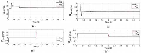
In this section the proposed hybrid controller is simulated on the IEEE 33 distribution system. For the purpose of comparison, the SOP locations are the same as those studied in the conventional controller of the previous section. The proposed method is based on the block diagram of Figure 7. Figure 13 (a) examines the tracking performance of the DC voltage controller at VSC 25, when the hysteresis controller is used for VSC 29. Prior to, $t=0.2\,\, \mathrm{sec}$, the controller has identical response as that presented in section 5.1 above. When VSC 29 is switched ON, the DC voltage controller shows insignificant change in the tracking performance, which can practically be considered as no change.
The same conclusion can be drawn for the tracking of, $Q_{v s c-25}$. Hence, an important conclusion is that a change of con trol approach for VSC 29 has practically no effect on the PI controllers performance for VSC 25 . Real and reactive power tracking for the hysteresis controller shows very good tracking of the actual powers, $P_{v s c-29}$ and $Q_{v s c-29}$, compared to its optimized reference value, $P_{r e f-29}$ and $Q_{r e f-29}$, as its evident from Figure 13 (c) and (d). Fast response is observed with very small overshoot compared to the PI based controllers for this converter at the same location studied in section 5.1.Moreover, very small to no ripple is seen in the response. In terms of tracking error, $P_{v s c-29}$ shows nearly very insignificant error whereas, $Q_{v s c-29}$, shows a small steady state error. It is clear that with this hysteresis controller the tracking profile is more smoother compared to the PI case. Smooth tracking can positively impact both load feeders situated on buses 25 and 29 of the distribution system.
Figure 14 shows the voltage profile at bus bars of connection and two bus bars from a relatively distant radials relative to the SOP location. The same distant buses are selected as in the conventional PI controller, which are bus bar 4 & 5.
Figure 13. Simulation results of Hybrid controller for SOP location (25-29): (a) dc side voltage, (b) reactive power response of VSC-25, (c) active power response of VSC-29 and (d) reactive power response of VSC-29
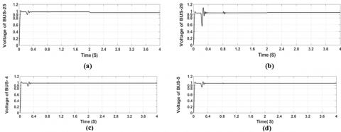
Figure 14. Simulation results of bus-bar voltages of using hybrid controller at: (a) bus 25, (b) bus 29, (c) bus 4 and (d) bus 5
Figure 15. Simulation results of hybrid controller at SOP location of (8-21): (a) dc side voltage, (b) reactive power response of VSC 8, (c) active power response of VSC2 and (d) reactive power response of VSC 21
Figure 16. Bus-bar voltage profiles using hybrid controller at: (a) bus 8, (b) bus 21, (c) bus 4 and (d) bus 5
Table 3. Comparison of conventional PI versus proposed hybrid SOP controllers
|
Point of Comparison |
PI based Controller |
Hybrid Controller |
||
|
Tracking Errors (P.U) |
Location 25-29 |
Location 8-21 |
Location 25-29 |
Location 8-21 |
|
DC voltage |
0.0332 |
0.0292 |
0.0021 |
0.0024 |
|
Reactive power of $V S C_i$ |
0.0014 |
0.0014 |
0.0097 |
0.0097 |
|
Real power of $V S C_i$ |
0.0027 |
5.817e-04 |
1.479e-07 |
4.468e-07 |
|
Reactive power of $V S C_i$ |
0.0012 |
7.938e-05 |
6.125e-07 |
1.36e-08 |
|
Ripple in controlled signals, $Q_{v s c-i}, P_{v s c-j} \& Q_{v s c-j}$ |
Clear oscillations in all actual signals of the SOP optimal operating points powers, specially, $P_{v s c-j}$ & $Q_{v s c-j}$ |
No oscillations are seen in all actual power signals of the converter that is controlled by the hysteresis approach, i.e. $P_{v s c-j}$ & $Q_{v s c-j}$ |
||
|
Effect of switching action on voltages at bus-bars of connection |
Clear switching action is reflected in the voltage profile of the $i^{t h}$ & $j^{t h}$ bus-bars at which the PI controlled converters is connected. |
No switching actions is observed in the voltage profile of the $j^{t h}$ bus-bar at which the hysteresis controlled converter is connected. |
||
|
Effect of switching action on bus-bars at distant location from SOP connection |
Some oscillations are seen in those distant buses, especially after $t=2\,\, \mathrm{sec}$ when the $j^{t h}$ converter is triggered. |
No oscillations are seen even after, $t=2\,\, \mathrm{sec}$ when the $j^{t h}$ bus-bar converter is switched on. |
||
|
Overshoot in actual signals |
Large overshoots in actual power signals for both converters in the PIs frame. |
No overshoot is seen in real and reactive actual powers for the converter at the $j^{t h}$ bus-bar. |
||
|
Effect of SOP converters on consumer load feeders, in-terms of overshoots and ripples |
Can be significant due to, over shoots in real/reactive power, and ripples in bus-bar voltages. |
Insignificant due to no overshoots in the control response and voltage ripples. |
||
|
Controller Components |
||||
|
Number of PIs controllers |
8 |
5 |
||
|
Number of parameters required to be tuned |
16 |
10 |
||
Inspection of results show the voltage profile suffers less ripple in the proposed hybrid controller compared to the conventional case. This is evident from Figure 14 (a) and (b) at both buses of connection. The transient response, however is different in terms of the voltage dip that occurs at bus 25 which supplies positive real power. Here, the voltage is instantaneously reduced to about 0.9 P.U compared to a dip of less than 0.6 P.U in the PI approach as depicted in Figure 10 (a). Hence, the transient effect in the voltage of the converter that operates as a rectifier is less compared to the conventional case. At bus 29 , the voltage profile, shown in Figure 14 (b), shows a relatively large momentarily dip before quickly reaching steady state. At the time of switching VSC 29 , at $t=$ $2\,\, \mathrm{sec}$, the bus voltage rises to new value with small delay as depicted Figure 14 (b). This is attributed to the time taken by the hysteresis controller to track the reference optimum real power, $P_{v s c-29}$, since this power is implicitly tracked through first calculating the dq reference currents, defined by Eq. (25) & (26), followed by conversion to stationary abc frame. A time interval is needed for the calculations and conversion to be performed. Voltage at bus 25, Figure 14 (a), also experience this delay due to the interaction of system dynamics. At the distant buses, it is interesting to note that at the instant of converter switching, specially converter at bus bar 25 , the voltage at both buses drops to about 0.9 P.U compared to about $0.8\,\, \mathrm{P}$ U in the conventional PI controller.
Hence, the hybrid controller yields less transient effects on the relatively distant buses compared to the PI controller. Voltage profile at these distant buses reveals no switching oscillations as shown in Figure 14 (c) & (d) compared to the PI based controllers case for the same buses that were shown in Figure 10 (c) and (d).
The proposed hybrid control method is further implemented for an SOP connection at buses 8-21 which is an open point in the distribution system. Optimal values of real/reactive powers of VSC21 obtained from the PSO algorithm that were used in the PI approach is implemented here through the hybrid controller. Figure 15 (a), (b), (c) and (d), show the DC tracking performance, $Q_{v s c-8}, P_{v s c-21}$, and $Q_{v s c-21}$ tracking respectively. Based on the optimization results, $P_{v s c-21}$ is positive, which is tracked very satisfactory through the hysteresis controller. The same is also seen for reactive powers at both buses of connection. Figure 16 (a), (b), (c) and (d), shows a similar response of the bus-bars voltage profile at the points of connection and distant radials as in location 25-29. Since both locations show similar response, this confirms the feasibility of the hybrid method for any SOP location decided by the distribution system operator.
5.3 Comparison between PI and hybrid controllers for converters of a soft open point device
In this section a comparison is provided to highlights the main difference between an SOP system controlled by the conventional PI and hybrid approach.
First, as far as the tracking efficiency is concerned, the hybrid approach shows a more accurate, less ripple tracking.
The tracking accuracy is judged based on calculation of the mean square error (MSE) between the reference settings, obtained through the PSO algorithm for real/reactive powers, and the actual values from the controller. The tracking errors of real power for $V S C_j$ for location $25-29$ is about 0.0027 by using PI controller while for the same location but by using hybrid controller the tracking errors of real power for $V S C_j$ is very small about $1.479 \mathrm{e}-07$. As for the second location, that is, SOP 8-21 the tracking errors of real power for $V S C_j$ is about $5.817 \mathrm{e}-04$ by using PI controller while for the same location but by using hybrid controller the tracking errors of real power for $V S C_j$ is about $4.468 \mathrm{e}-07$, and so for the remaining parameters of DC voltage, reactive power of $V S C_j / j$ and real power of $V S C_j$, it clearly shows the efficiency of the hybrid controller in accurately tracking and reducing the errors between the reference values and the measured values. for the ripples in controlled signals the hybrid controller demonstrate that nearly no ripples are seen in controlled actual signals.
Furthermore, other features of the hybrid controller is illustrated in Table 3. Here, the error for the tracking performance of the hybrid approach is evaluated after $t \geq$ $2\,\, \mathrm{sec}$, for all locations where the SOP is connected. The hybrid method shows considerable mitigation in the bus-bar voltage profiles as far as the oscillations is concerned. Moreover, nearly no overshoot is observed in the $j^{\text {th }}$ converter real and apparent powers response which will positively impact the operation of the distribution system in terms of avoiding nuisance activation of protection devices.
For example at location 25-29, the actual real power at bus 29 overshoots to 0.3 P.U as the converter is triggered when the conventional PI controller is employed as evident from Figure 9c. This is compared to nearly no overshoot in the hybrid controller case as seen in Figure 13 (c).
Work in this paper presents the controls of SOP devices in the environment of an electrical distribution system. A proposed approach is presented that employs two different controls methods for each converter of the SOP. Therefore, the overall control is hybrid in nature. A PSO based search algorithm is first suggested that computes the optimal operating power points of the SOP corresponding to the minimization a specific cost function. These computed optimal points are utilized as reference settings in the suggested hybrid approach. Compared to the conventional PI based controllers, the hybrid method has less tracking error, nearly no overshoots in real and reactive power actual signals of the converter. For example the SOP converter at bus-bar 29, an overshoot of 0.3 P.U is observed in the actual real power with PI controls compared to no significant overshoot when the same converter is controlled using the hysteresis approach. Furthermore, the hybrid approach revels less oscillations in voltage profiles at the bus-bars of connection and some distant bus-bars of other radials. These aforementioned features of the hybrid approach increases the reliability of the distribution system in terms of avoiding false tripping of protection devices and a less oscillatory bus bar voltage profile, where consumer loads are fed.
|
SOP |
Soft Open Point |
|
PSO |
Particle Swarm Optimization algorithm |
|
NOP |
Normally Open Points |
|
VSC |
Voltage source converter |
|
$V S C i S W$ |
Switching signals of converter at bus i |
|
$V S C j S W$ |
Switching signals of converter at bus j |
|
PI |
Proportional Integral controller |
|
$P_{V S C-i}$ |
Real power of converter at bus i |
|
$Q_{V S C-i}$ |
Reactive power of converter at bus i |
|
$P_{V S C-j}$ |
Real power of converter at bus j |
|
$Q_{V S C-j}$ |
Reactive power of converter at bus j |
|
$P_{r e f-j}$ |
Reference real power of converter at bus i |
|
$Q_{ {ref-i }}$ |
Reference reactive power of converter at bus i |
|
$P_{ {ref-i }}$ |
Reference real power of converter at bus j |
|
$Q_{r e f-j}$ |
Reference reactive power of converter at bus j |
|
$i_d \& i_q$ |
Currents of rotating frame |
|
$i_\alpha \& i_\beta$ |
Currents of stationary frame |
|
$i_{ {drefi } / j}$ |
Reference d-axis current for i or j bus converter |
|
$i_{ {qref } i / j}$ |
Reference q-axis current for i or j bus converter |
|
$\mathrm{V}_{\mathrm{dmod} \mathrm{i} / \mathrm{i}}$ and $\mathrm{V}_{\mathrm{qmod} \mathrm{i} / \mathrm{i}}$ |
Modulating voltage of dq frame at bus i or j |
|
$V_{d i / j} \& V_{q i / j}$ |
Voltage of bus i or j in dq frame |
|
$C, V_{D C}$ and $i_C$ |
Equivalent value of capacitance, dc voltage and current of capacitor |
|
$\widetilde{V_{D C}^2}$ |
Deviation in square of DC voltage |
|
$\widetilde{P}_l$ |
Deviation in power injected at bus i |
|
$P_{i o}$ |
Steady state point of real power at bus i |
|
$G_{P i-v}(s)$ |
Transfer function of the PI voltage controller |
|
$G_{\text {in-loop }}(s)$ |
Closed loop transfer function of the power controller (or current controller) |
|
MSE |
Mean Sequar Error |
Bus and line data of IEEE 33 Bus system [31] are noted in Table A1 below.
Table A1. Bus and line data of IEEE 33
|
From Bus |
To Bus |
R (ohms) |
X (ohms) |
P (KW) |
Q (KVAR) |
|
1 |
2 |
0.0922 |
0.0470 |
100 |
60 |
|
2 |
3 |
0.4930 |
0.2511 |
90 |
40 |
|
3 |
4 |
0.3660 |
0.1864 |
120 |
80 |
|
4 |
5 |
0.3811 |
0.1941 |
60 |
30 |
|
5 |
6 |
0.8190 |
0.7070 |
60 |
20 |
|
6 |
7 |
0.1872 |
0.6188 |
200 |
100 |
|
7 |
8 |
0.7114 |
0.2351 |
200 |
100 |
|
8 |
9 |
1.0300 |
0.7400 |
60 |
20 |
|
9 |
10 |
1.0440 |
0.7400 |
60 |
20 |
|
10 |
11 |
0.1966 |
0.0650 |
45 |
30 |
|
11 |
12 |
0.3744 |
0.1298 |
60 |
35 |
|
12 |
13 |
1.4680 |
1.1550 |
60 |
35 |
|
13 |
14 |
0.5416 |
0.7129 |
120 |
80 |
|
14 |
15 |
0.5910 |
0.5260 |
60 |
10 |
|
15 |
16 |
0.7463 |
0.5450 |
60 |
20 |
|
16 |
17 |
1.2890 |
1.7210 |
60 |
20 |
|
17 |
18 |
0.7320 |
0.5740 |
90 |
40 |
|
2 |
19 |
0.1640 |
0.1565 |
90 |
40 |
|
19 |
20 |
1.5042 |
1.3554 |
90 |
40 |
|
20 |
21 |
0.4095 |
0.4784 |
90 |
40 |
|
21 |
22 |
0.7089 |
0.9373 |
90 |
40 |
|
3 |
23 |
0.4512 |
0.3083 |
90 |
50 |
|
23 |
24 |
0.8980 |
0.7091 |
420 |
200 |
|
24 |
25 |
0.8960 |
0.7011 |
420 |
200 |
|
6 |
26 |
0.2030 |
0.1034 |
60 |
25 |
|
26 |
27 |
0.2842 |
0.1447 |
60 |
25 |
|
27 |
28 |
1.0590 |
0.9337 |
60 |
20 |
|
28 |
29 |
0.8042 |
0.7006 |
120 |
70 |
|
29 |
30 |
0.5075 |
0.2585 |
200 |
600 |
|
30 |
31 |
0.9744 |
0.9630 |
150 |
70 |
|
31 |
32 |
0.3105 |
0.3619 |
210 |
100 |
|
32 |
33 |
0.3410 |
0.5302 |
60 |
40 |
|
8 |
21 |
2.0000 |
2.0000 |
|
|
|
9 |
15 |
2.0000 |
2.0000 |
|
|
|
12 |
22 |
2.0000 |
2.0000 |
|
|
|
18 |
33 |
0.5000 |
0.5000 |
|
|
|
25 |
29 |
0.5000 |
0.5000 |
|
|
[1] Hung, D.Q., Mithulananthan, N., Bansal, R.C. (2014). Integration of PV and BES units in commercial distribution systems considering energy loss and voltage stability. Applied Energy, 113: 1162-1170. https://doi.org/10.1016/j.apenergy.2013.08.069
[2] Mu, Y., Wu, J., Jenkins, N., Jia, H., Wang, C. (2014). A spatial–temporal model for grid impact analysis of plug-in electric vehicles. Applied Energy, 114: 456-465. https://doi.org/10.1016/j.apenergy.2013.10.006
[3] Savić, A., Đurišić, Ž. (2014). Optimal sizing and location of SVC devices for improvement of voltage profile in distribution network with dispersed photovoltaic and wind power plants. Applied Energy, 134: 114-124. https://doi.org/10.1016/j.apenergy.2014.08.014
[4] Chen, T.H., Huang, W.T., Gu, J.C., Pu, G.C., Hsu, Y.F., Guo, T.Y. (2004). Feasibility study of upgrading primary feeders from radial and open-loop to normally closed-loop arrangement. IEEE Transactions on Power Systems, 19(3): 1308-1316. https://doi.org/10.1109/TPWRS.2004.831263
[5] Okada, N., Kobayashi, H., Takigawa, K., Ichikawa, M., Kurokawa, K. (2003). Loop power flow control and voltage characteristics of distribution system for distributed generation including PV system. In 3rd World Conference on Photovoltaic Energy Conversion, Osaka, Japan, pp. 2284-2287.
[6] Bloemink, J.M., Green, T.C. (2010). Increasing distributed generation penetration using soft normally-open points. In IEEE PES General Meeting, Minneapolis, MN, USA, pp. 1-8. https://doi.org/10.1109/PES.2010.5589629
[7] Bloemink, J.M., Green, T.C. (2013). Benefits of distribution-level power electronics for supporting distributed generation growth. IEEE Transactions on Power Delivery, 28(2): 911-919. https://doi.org/10.1109/TPWRD.2012.2232313
[8] Bloemink, J.M., Green, T.C. (2011). Increasing photovoltaic penetration with local energy storage and soft normally-open points. In 2011 IEEE Power and Energy Society General Meeting, Detroit, MI, USA, pp. 1-8. https://doi.org/10.1109/PES.2011.6039561
[9] Tang, C.Y., Chen, Y.F., Chen, Y.M., Chang, Y.R. (2015). DC-link voltage control strategy for three-phase back-to-back active power conditioners. IEEE Transactions on Industrial Electronics, 62(10): 6306-6316. https://doi.org/10.1109/TIE.2015.2420671
[10] Hussain, H.A. (2023). Enhanced control of back-to-back converters in wind energy conversion systems using two-degree-of-freedom (2DOF) PI controllers. Electronics, 12(20): 4221. https://doi.org/10.3390/electronics12204221
[11] Babu, B.P., Indragandhi, V. (2020). Analysis of back to back (BTB) converter control strategies in different power system Applications. Materials Science and Engineering, 906(1): 012016. https://doi.org/10.1088/1757-899X/906/1/012016
[12] Hannan, M.A., Hussin, I., Ker, P.J., Hoque, M.M., Lipu, M.H., Hussain, A., Blaabjerg, F. (2018). Advanced control strategies of VSC based HVDC transmission system: Issues and potential recommendations. IEEE Access, 6: 78352-78369. https://doi.org/10.1109/ACCESS.2018.2885010
[13] Awahab. (2024). VSC based HVDC system. https://www.mathworks.com/matlabcentral/fileexchange/53232-vsc-based-hvdc-system.
[14] Jafari, H., Mahmoudi, M., Fatehi, A., Naderi, M.H., Kaya, E. (2018). Improved power sharing with a back-to-back converter and state-feedback control in a utility-connected microgrid. In 2018 IEEE Texas Power and Energy Conference (TPEC), College Station, TX, USA, pp. 1-6. https://doi.org/10.1109/TPEC.2018.8312106
[15] Zhang, Z., Wang, F., Sun, T., Rodriguez, J., Kennel, R. (2015). FPGA-based experimental investigation of a quasi-centralized model predictive control for back-to-back converters. IEEE Transactions on Power Electronics, 31(1): 662-674. https://doi.org/10.1109/TPEL.2015.2397695
[16] Souza, I.D., de Almeida, P.M., Fogli, G.A., Barbosa, P.G., Ribeiro, P.F. (2021). Multivariable optimal control applied to a back-to-back power converter. IEEE Transactions on Industrial Electronics, 69(9): 9406-9418. https://doi.org/10.1109/TIE.2021.3114748
[17] Blaabjerg, F. (Ed.). (2018). Control of Power Electronic Converters and Systems: Volume 2 (Vol. 2). Academic Press.
[18] Putri, A.I., Rizqiawan, A., Rozzi, F., Zakkia, N., Haroen, Y., Dahono, P.A. (2016). A hysteresis current controller for grid-connected inverter with reduced losses. In 2016 2nd International Conference of Industrial, Mechanical, Electrical, and Chemical Engineering (ICIMECE), Yogyakarta, Indonesia, pp. 167-170. https://doi.org/10.1109/ICIMECE.2016.7910446
[19] Julius, C.N.A., Muhammad, L.N., Daniyal, H., Jaalam, N., Abdullah, N.R.H., Ghani, S.A. (2019). A comparative study of hysteresis current controller and PI controller in grid-connected inverter. International Journal of Advanced Trends in Computer Science and Engineering, 8(6): 3182-3187.
[20] Qi, Q., Wu, J., Long, C. (2017). Multi-objective operation optimization of an electrical distribution network with soft open point. Applied Energy, 208: 734-744. https://doi.org/10.1016/j.apenergy.2017.09.075
[21] Cao, W., Wu, J., Jenkins, N., Wang, C., Green, T. (2016). Operating principle of soft open points for electrical distribution network operation. Applied Energy, 164: 245-257. https://doi.org/10.1016/j.apenergy.2015.12.005
[22] Long, C., Wu, J., Thomas, L., Jenkins, N. (2016). Optimal operation of soft open points in medium voltage electrical distribution networks with distributed generation. Applied Energy, 184: 427-437. https://doi.org/10.1016/j.apenergy.2016.10.031
[23] Bloemink, J.M. (2013). Distribution-level power electronics: Soft open-points. Doctoral Dissertation, Imperial College London.
[24] Bajracharya, C., Molinas, M., Suul, J.A., Undeland, T.M. (2008). Understanding of tuning techniques of converter controllers for VSC-HVDC. In Nordic Workshop on Power and Industrial Electronics (NORPIE/2008), June 9-11, 2008, Espoo, Finland, pp. 1-8.
[25] Kennedy, J., Eberhart, R. (1995). Particle swarm optimization. In Proceedings of ICNN'95-International Conference on Neural Networks, Perth, WA, Australia, pp. 1942-1948. https://doi.org/10.1109/ICNN.1995.488968
[26] Cao, W., Wu, J., Jenkins, N. (2014). Feeder load balancing in MV distribution networks using soft normally-open points. In IEEE PES Innovative Smart Grid Technologies, Europe, Istanbul, Turkey, pp. 1-6. https://doi.org/10.1109/ISGTEurope.2014.702887
[27] Zimmerman, R.D., Murillo-Sánchez, C.E., Thomas, R.J. (2010). MATPOWER: Steady-state operations, planning, and analysis tools for power systems research and education. IEEE Transactions on Power Systems, 26(1): 12-19. https://doi.org/10.1109/TPWRS.2010.2051168
[28] Yazdani, A., Iravani, R. (2010). Voltage-Sourced Converters in Power Systems: Modeling, Control, and Applications. John Wiley & Sons.
[29] Mtonga, T., Kaberere, K.K., Irungu, G.K. (2023). Optimal network reconfiguration for real power losses reduction. In the IEEE 33-Bus Radial Distribution System, Authorea Preprints, pp. 1-6. https://doi.org/10.36227/techrxiv.19747447.v1
[30] Stoppato, A., Cavazzini, G., Ardizzon, G., Rossetti, A. (2014). A PSO (particle swarm optimization)-based model for the optimal management of a small PV (Photovoltaic)-pump hydro energy storage in a rural dry area. Energy, 76: 168-174. https://doi.org/10.1016/j.energy.2014.06.004
[31] Kumar, D., Agrawal, S. (2013). Load flow solution for meshed distribution networks. BSC. National Institute of Technology, Rourkela (ODISHA), India.