Suryachandra Palli | Ghamya Kotapati![]() | Kranthi Kumar Lella
| Kranthi Kumar Lella![]() | Jagadeeswara Rao Palisetti
| Jagadeeswara Rao Palisetti![]() | Dorababu Sudarsa
| Dorababu Sudarsa![]() | Syed Ziaur Rahman
| Syed Ziaur Rahman![]() | Ramesh Vatambeti*
| Ramesh Vatambeti*![]()
© 2024 The authors. This article is published by IIETA and is licensed under the CC BY 4.0 license (http://creativecommons.org/licenses/by/4.0/).
OPEN ACCESS
Services for AI tasks have garnered a lot of attention as an integral aspect of intelligent services in the new era. However, implementing such a system in a stable and distributed manner, while simultaneously coordinating the use of cloud computing and remote edge devices, is challenging due to the pressing need for energy and computing resources. The primary contribution of this study lies in the development of a distributed co-inference architecture that harnesses the collective intelligence of interconnected agents to optimize traffic flow in real-time. By combining Q-learning with enhanced deep learning, our approach enables traffic signals and routing decisions to adapt dynamically to changing traffic patterns and environmental conditions. The security, responsiveness, and dependability of intelligent systems deployed close to end-users are improved by deploying deep learning systems. Another critical aspect where latency and accuracy in models are traded off is deep learning model optimization. Finding the best offloading policy and model for deep learning services requires an end-to-end decision-making solution that takes into account computation-communication problems. This study presents a holistic network optimization approach for scheduling AI services based on artificial intelligence. By adjusting for differences in computational resources and network congestion, the suggested deep Q-learning technique maximizes the throughput of AI tasks in general. This research introduces a virtual queue for analyzing the system's Lyapunov stability and employs a multi-hop Directed Acyclic Graph (DAG) to explain Q-learning of Reinforcement learning-based co-inference network topology. To optimize the total task processing rate, the study develops an Optimized self-adaptive glow worm swarm optimization method (SA-GSO) based on deep Q-learning. It then proposes a priority-based data forwarding approach for efficiency. The study concludes by simulating the distributed co-inference system's platform. We attest to the superiority of our idea by comparing it to other standards.
Q-Learning, deep learning, reinforcement learning agent, co-inference
Thanks to an ongoing mutual benefit, artificial intelligence (AI) has made tremendous strides in the last 20 years, giving rise to what is now known as AI-enabled IoT and realizing the goal of pervasive intelligence [1, 2]. A new network architecture can be built and effectively used with the help of methods and knowledge created under the Internet of Things (IoT) paradigm. This architecture will consist of interconnected ambient sensing devices, such as embedded devices and mobile phones, that are resource-constrained [3]. These devices are often called user equipment (UE) in the relevant literature. In this area, the main focus has been on creating and implementing more efficient and faster network infrastructures and building more precise sensing platforms. Massive improvements in these systems' sensing capabilities have made it possible to gather and store vast amounts of data, enabling ever-more-advanced artificial intelligence techniques, ranging from classic ML approaches to more modern deep learning (DL) tactics, opening up vast possibilities for a 'smart' life [4].
Deep neural networks (DNNs) have proven their power and achieved great success in many application domains, including smart farming and smart healthcare [5]. New degrees of accuracy in the supplied findings have been achieved by the utilization of deep learning algorithms and large data collection made possible by utilizing the sensors incorporated in these systems [6]. Training the networks and forming inferences now require more computational and memory resources, but the accuracy is worth it [7]. For most use cases in the typical application areas of IoT schemes, time is of the essence, and real-time prediction presentation is expected. Inference, in particular, involves more than just multiple processed DNN outputs; it involves both devices [8].
To handle AI tasks efficiently and rapidly, AI-based services often upload raw data straight to the cloud, which is necessary because deep learning models require a lot of computing power [9]. Since the terminal lacks the computational capability to complete a service request alone, the raw data is transmitted to the cloud [10]. Network delay, data loss, and security threats are all possibilities when data is delivered to the cloud, and AI processes it. The cloud then provides the output to the terminal. Luckily, DNN-based co-inference computation uses much less energy and has much less latency because the edge device supplies additional processing resources to allow distributed computing [11]. Central to this concept is the idea of using shallow processing to reduce computationally huge raw data from low-computational devices into smaller features, which can subsequently be transmitted to a higher layer for additional processing.
For reasons like big data capacity and privacy issues, the raw data is handled by the front of neural networks organized in edge strategies. The images, which are data, are then sent to the edge layer processing [12]. The final section of the neural network labels the characteristics that are transferred to the cloud after compression of the unlabeled output. For inference procedures that require a lot of processing power but don't require a huge amount of data, the cloud layer comes in handy. For artificial intelligence applications like face recognition and autonomous driving, the user's terminal receives the final tagged features [13]. Several supports, including processing power of the device, transmission quality of the network, and resolution precision, are typically needed for this operation. More effective, energy-friendly, and spontaneous scheduling of AI tasks using network resources is one of the key issues.
One of the challenges in developing an integrated solution is combining heterogeneous devices on one platform. These devices' capabilities, such as transmission bandwidth and computing power, are on the rise in urban IoT systems and smart devices [14]. Processing power, as a result of energy-efficient architectural principles, must cater to consumers' demands in real-time while exhibiting increased latency demands. Intelligent optimization of platform resources, including computation, communication, and cache resources, is the primary goal of this research. Classical convex optimization procedures also become inefficient when it comes to scheming a comprehensive plan in a limited amount of time due to the increasing number of terminal devices [15].
An optimization paradigm was designed to schedule the AI co-inference services across many terminal devices, thus enhancing the overall quantity of DNN jobs. This paradigm was used to tackle the aforementioned problem. Because of the demands of these huge devices, this research takes into account the possible difficulties that may arise from the unequal distribution of transmission and computation resources. In recent years, the integration of Artificial Intelligence (AI) techniques into various domains has revolutionized the way we tackle complex problems and optimize system performance. In transportation systems, AI-powered solutions offer promising opportunities to enhance traffic management, reduce congestion, and improve overall efficiency. However, deploying AI services in real-world traffic environments poses significant challenges, particularly in achieving scalability, adaptability, and robustness.
Traditional traffic management systems often rely on pre-defined rules or centralized control mechanisms to regulate traffic flow and optimize signal timings. While effective to some extent, these approaches struggle to cope with the dynamic and unpredictable nature of real-time traffic conditions. Moreover, centralized architectures can become bottlenecks, limiting scalability and resilience in large-scale traffic networks.
The emergence of distributed AI presents a compelling alternative, offering the potential to overcome many of these limitations. By decentralizing decision-making processes and distributing intelligence across interconnected agents, distributed AI enables more adaptive and responsive traffic control mechanisms. This paradigm shift not only enhances scalability and fault tolerance but also fosters collaboration and coordination among traffic management entities.
However, implementing AI services in a distributed manner comes with its own set of challenges. Firstly, ensuring synchronization and consistency among distributed agents while maintaining real-time responsiveness is non-trivial, especially in dynamic traffic environments. Secondly, effective communication and information exchange between decentralized components are crucial for achieving collective intelligence and coordinated decision-making
Moreover, distributed AI systems must contend with issues of privacy, security, and data integrity, particularly in the context of sensitive traffic data and communication protocols. Ensuring trust and compliance with regulatory requirements is paramount to the successful deployment of distributed AI in traffic management applications.
Here is how the remainder of the paper is organized: Section 2 presents the related work; The organization model is shown in Section 3; The projected Q-learning is discussed in Section 4; the results analysis is obtainable in Section 5, and lastly, the study activity is summarized in Section 6.
In order to uncover neuro-physiological patterns connected to Situation Awareness (SA) and hierarchically recognize Air Traffic Controllers' (ATCOs) SA loss associated with workload concerns, Li et al. [16] suggest a two-stage analytical process that utilizes EEG and eye-tracking data. First, we used SA-probe tests to gather behavioral and physiological data in a simulated air traffic control (ATC) radar-monitoring experiment with varying task loads. Then, we measured the participants' perceived workloads using the NASA scale. In our research, divided into two phases, we used the Gaussian Mixture Model to analyze task performance behavioral data and calculate the sample's SA. In the second phase, we classified the samples according to their perceived workloads using NASA-TLX ratings. Based on the results of Phase I, we annotated the physiological data. In Phase II, we used fast Fourier transform and Hilbert transform to extract the physiological feature base. Finally, we used linear discriminant analysis to extract the core features, which we then used to train multiple classifiers. This allowed us to achieve our purposes. The results demonstrated that SA loss's neuro-physiological behaviors varied between low and high workloads. The findings of a leave-one-out validation displayed that the optimal performance for 1-level classification of high/low SA was 76.1%, and for 2-level classification of low SA linked with high workload, it was 82.7%.
By utilizing a dataset and data collected from our trial flights, Çelik and Eren [17] sought to extract a flight fingerprint using several machine learning approaches. We used manifold learning algorithms to minimize multidimensional UAV sensor data to determine the individual flying pattern. A comparison was conducted to determine the optimal manifold strategy that achieves the maximum classification accuracy (CA). Various manifold types and categorization algorithms are used to compare their performances. The resulting manifold is further confirmed using classification techniques and utilized as a flight fingerprint. For the purpose of dimension reduction, a number of unsupervised manifold learning algorithms were implemented. Various supervised machine learning algorithms were evaluated for flight fingerprint classification, including k-Nearest Neighbors (k-NN), Adaboost, Neural Network, Bayes, and others. Combining the t-SNE manifold with the k-NN classification yields the best results in terms of classification accuracy. Production line performance testing, analysis, anomaly identification, pilot performance monitoring, and drone efficiency tracking are just a few of the numerous potential uses for the retrieved fingerprint.
A Non-Divergent Traffic Management Scheme (NDTMS) was proposed by Manimurugan and Almutairi [18] to enhance roadside driving for both users and automobiles. Using environmental navigation data, this scheme can identify and categorize nearby vehicles, people, and obstacles. Pervasive computing technologies aid in non-deviating smooth application assistance by combining two inputs into density statistics provided by the input data. Neighbor data extraction aids feature matching and traffic reduction. Classifier learning links to application-specific needs, addressing the problem of data mishandling for traffic management. Using a combination of data from navigation, alarms, and communications, this pervasive computing technology enables exact traffic management.
In order to automatically and continuously distinguish diverse types of unknown traffic generated by different attack tools in contradiction of SCADA in real-time, Sheng et al. [19] have proposed a self-growing ATC model that is based on a novel density-based heuristic clustering algorithm. To further enhance ATC performance, an efficient technique of representing SCADA system traffic is suggested. Further, the suggested strategy is tested by a battery of experiments dataset that includes the SCADA dataset and the ICS dataset. In the critical scenario of just regular SCADA network traffic, the experimental findings demonstrate that the suggested technique surpasses current state-of-the-art ATC algorithms.
An evolutionary feature selection model and a Convolutional Neural Network (CNN) are combined in a hybrid model for vehicle classification suggested by Alghamdi et al. [20]. Sports cars, luxury cars, and hybrid powerhouse SUVs are just a few of the eight types of vehicles that the suggested model might classify. The data utilized in this study comes from the Stanford vehicle dataset, which includes nearly 196 different types of vehicles. Once the necessary data preparation and preprocessing processes have been completed, the next step is to use a pre-trained VGG16 model to learn and extract deep features from the input photos. The final fully connected layer of VGG16 is used to extract these features, and a Genetic Algorithm (GA), an optimization model inspired by nature and based on evolution, is used to carry out the feature optimization phase. Several support vector machine (SVM) kernels are used for the classification, with Cubic SVM achieving a 99.7 percent accuracy, surpassing all other kernels and performing better than previous efforts.
In order to identify photos according to the traffic density and offer driving assistance, Mane et al. [21] suggest using a customized convolutional neural network (CCNN) on traffic images. Using footage from deployed cameras, the paper's proposed system may track traffic and assign it a high, medium, or low priority based on the present scenario. With this model as a guide, we may better teach expert systems about traffic density in different locations and make informed decisions about traffic regulation. To achieve higher accuracy, the training process is parallelized and complicated using an NVIDIA graphics processing unit (GPU). A real-time dataset of traffic footage from Pune city and film from highway CCTVs in Seattle, WA, acquired from Washington State, is used to assess the performance of the projected system. The findings of the experiment estimate the traffic density with a level of accuracy of up to 99.6 percent, categorizing it as high, medium, or low depending on the current traffic. The findings provided by the current algorithms are much inferior to the achieved testing accuracy.
After that, the study will provide the suggested system's overall architecture and explain the formulas, data transfer, inference processing, and capacity limits in detail.
3.1 System framework
Distributed deep learning systems typically have four levels of architecture: an input layer that is based on the real world, a pre-processing layer that uses terminal devices, an edge-based inference layer that uses devices in the network's periphery, and a cloud-based inference layer that uses devices in the cloud. The integration of Artificial Intelligence (AI) techniques into transportation systems holds immense promise for addressing the challenges of modern urban mobility. With cities facing escalating congestion, pollution, and inefficient resource utilization, there is an urgent need for innovative solutions to optimize traffic flow, reduce travel time, and enhance overall transportation efficiency. In this context, the adoption of AI-powered traffic management systems has emerged as a pivotal strategy to tackle these pressing issues.
However, while AI offers unprecedented capabilities for optimizing traffic control, traditional centralized approaches often struggle to adapt to the dynamic and complex nature of urban traffic environments. Moreover, as cities continue to expand and evolve, the scalability and resilience of existing traffic management systems become increasingly strained. In response, there is growing interest in leveraging distributed AI architectures to overcome these limitations and achieve more adaptive and efficient traffic control mechanisms.
Raw data layer: Internet of Things apps incorporate a variety of AI-based services, such as visual data, speech data, and RGB images. Data aimed at artificial intelligence (AI) is typically larger before processing to achieve better inference accuracy. For example, the maximum bit depth for a video frame is 134891 B. The service latency is strongly correlated with the user experience when dealing with lesser amounts of voice data [22]. It is possible for a single co-inference image to exceed 1 Mb/time in size.
Local layer: In the first layer that processes the raw data, the Internet of Things (IoTs) is implanted with the shallow neural network. These gadgets help reduce the amount of transmission packets and point the way for future inference. Updated to neighboring edge devices, the processed data consists of unlabeled features. The devices at the edge of a network sometimes have less processing capacity, but they excel at transforming data contact.
Edge layer: Although they lack the computing power of the cloud, devices in the edge layer are more equipped to provision resources due to their involvement in the gateway. The system improves processing efficiency by reducing network congestion and optimizing the edge devices. It finds idle devices to synchronize with and computes the unmarked edge devices to upload further by optimizing computing resources. The last step in the inference process is for the edge device to upload the treated feature statistics to the cloud.
Cloud layer: The cloud's service capacity usually dictates the scheme's overall capacity. We take into account processing, which is prevalent in the current architecture of the IoT, in our study. Distributed computing structures can better balance computer resources, network resources, and device failures through the use of optimal algorithms [23]. Assuming sufficient bandwidth for feature data transfer to these clouds is a key assumption in this work [24].
Data preprocessing layer:
The data preprocessing layer processes and cleans the raw traffic data to prepare it for further analysis and modeling.
Tasks performed in this layer include data filtering, noise reduction, missing value imputation, and normalization.
Preprocessed data is formatted into appropriate input representations for subsequent analysis.
Limitations: Preprocessing techniques may introduce biases or loss of information, impacting the quality of input data for downstream tasks.
Feature extraction layer:
The feature extraction layer extracts relevant features from preprocessed traffic data using deep learning techniques, such as Convolutional Neural Networks (CNNs) and Recurrent Neural Networks (RNNs).
Features extracted may include spatial and temporal patterns, traffic flow dynamics, vehicle trajectories, and environmental factors.
Extracted features serve as input representations for the decision-making process in subsequent layers.
Limitations: The effectiveness of feature extraction may depend on the quality and diversity of training data, as well as the design of the deep learning models used.
Decision-making layer:
The decision-making layer incorporates Q-learning algorithms to optimize traffic control policies based on the extracted features and current traffic conditions.
Traffic control agents, such as traffic signal controllers or route planners, use Q-learning to learn optimal action-selection strategies for minimizing travel time, reducing congestion, and improving overall traffic flow.
Decisions made by traffic control agents are based on the Q-values learned through reinforcement learning and the current state of the traffic network.
Limitations: Q-learning may require extensive training and exploration to converge to optimal policies, and its performance may be affected by the complexity and stochasticity of traffic environments.
3.2 Networking and task processing
The research describes the data forwarding and task dispensation in the suggested structure using a graph as GðV; EÞ. The following is an explanation of our three-layer network architecture: we reflect terminal devices set as $N=\left\{1,2,3, \ldots, n_{\max }\right\}$, edge layer set as $M=\left\{1,2,3, \ldots, m_{\max }\right\}$ and cloud set as $K=\left\{1,2,3, \ldots, k_{\max }\right\}$, correspondingly. Thus, we have nodes on the map $v \in\{N, M, K\}=V$. Assuming that local device n includes both fixed and removable smart devices, we can say that: a mobile smart device has a stable link (edge) and is within the communication range r offered by the gateways. The same way around. A fixed edge connects the fixation device to the edge device. Suppose the gateway has a wired and wireless connection to a device in the local layer; device m in the edge layer serves a neighboring gateway with different bandwidth; and device n in the cloud layer offers the connection to device m in the edge layer in the third tier. Cloud k has a set amount of available computing and communiqué resources. In each time slot, the scheme completes the following three steps: generate tasks, convey is considered as $T=\left\{1,2,3, \ldots, t_{\max }\right\}$. The $\mathrm{N}$ terminal devices in the working state produce a set of packets $N^{\mathrm{g}}$. The M edge-layer device can receive upon to $M^{\mathrm{r}}$ packets. It makes a set of $M^{\mathrm{g}}$ packets congruently. The volume of the cloud is $K^r$. Additional tasks are put into the waiting queue. The broadcast links are measured as $E$, which are DAG. Single DAG $E_i \in E$ is measured as the temporal joining graph for period slot $t_{\mathrm{i}}$.
Therefore, the restraints of the data flow are considered as: the generation rate of AI tasks for node $v \in\{N, M\}$ is represented as $v^{\mathrm{g}}$. Arbitrary node's cohort rate is $v^g(t) \in$ $\left\{N_v^g\right\}$. The overall general rate is measured as $\bar{v}^g=$ $\sum_{t \in T} v^g(t)$, where incomplete by $\bar{v}^g \leq v_{\max }^g$. The getting rate for $v \in\{M, k\}$ should satisfy $v^g(t) \leq M_v^g$. Therefore, the output of node $v \in\{M, K\}$ is $v^{\mathrm{r}}$, where $v^r \leq M_v^r$ or $K_v^r$. Its consistent upper processing limit is $v_{\max }^r$.
3.3 Network activate
In the suggested setup, prior to dealing with AI tasks, the routing system activates the network in accordance with the following rules:
(1) Rearrange Network: The wireless node connects to the main network and makes a new link. Take the device out of graph G that isn't working.
(2) Link Initiation: From link set E, a matching link is triggered when a routing policy is set up.
(3) A data propagation: the routing method ensures that every link is used by sending out at least one packet. Furthermore, a link's capacity dictates the maximum number of packets that can be transmitted.
Suppose that $v^s(t)$ is the total amount of data that the node needs to broadcast at time t, including both externally generated jobs and its own initial data. The total rate of forwarding can be thought of as,
$\lim _{t \rightarrow \infty} \frac{v^s(t)}{t}=\bar{v}^s=\bar{v}^g+\bar{v}^q$ (1)
and $\bar{v}^q$ is the communicating data rate. Interim, the data dispensation speed in node $v_i$Q is renowned as
$\lim _{t \rightarrow \infty} \frac{v^r(t)}{t}=\bar{v}^r$ (2)
The common-sense conclusion is that after $\sum v^r$ is at its extreme and $\sum v^s$ is not. It means the current resource distribution policy is accomplished to make the optimal. When $\sum v^s$ is at its extreme, and $\sum v^r$ is not, it means additional copies are shaped to attain lower latency.
3.4 Scheme optimization goal
The data-generating device in the model is only concerned with the final destination of the task up to the point where it is chosen in the subsequent layer. Network congestion and the processing capacity of the destination determine the data forwarding timing. Here, we assume the destination node $v \in$ $\{N, M\}$ is denoted as $D_{\mathrm{v}}$.
If we ignore slightly capacity constraints, part of the links is full altogether the time. Presumptuous a scheduled route P, the data furtherance rate is measured as,
$v^s=\sum_{P_g \in P} v_g^s$ (3)
where, $v_g^s$ is the bringing degree of node v goes to -path $P_g$. The data rate for node v is the sum of each path $P_g \in P$. Assume $e_{i, j}$ is the volume of the edge node j, the regular forwarding rate is measured as
$\bar{v}_{i, j}^s=\sum_{P_g \in P} v_g \leq e_{i, j}$, where $P_g$ passes $i$ to $j$ (4)
It means the amount of entirely the path’s data proportion is incomplete by capacity [25]. The data rate $v_{\mathrm{i}, \mathrm{j}}$ corresponds to the edge from i to j. Thus, the aforementioned formula limits the maximum capacity for any bandwidth-limited network. Since only one node can handle segmented inference data at a time, no sibling distributed processing solution is available. With the node's data receiving bond taken into account, the total average getting rate is constrained by the node's processing capability.
$\sum_{P_g \in P} \bar{v}_g^r \leq \sum_{v \in\{M, K\}} \bar{v}^r$ (5)
The processing speed of the cloud determines the ultimate system output, which is the speed of feature data marking. Since the processing capability of the cloud exceeds that of the network, one of the obstacles to forwarding is the slowness of the network. The final output is affected by traffic caused by both local devices, although the volume of lower networks is ultimately limited by the capacity of end devices. Consequently, making the most of the cloud devices' whole receiving capacity is the difficulty. The primary impartial of this study is to outline an allocation policy that maximizes the clouds, as this is our optimization target.
$\begin{gathered}\max \bar{V}=\frac{1}{|T|} \sum_{t \in T} \sum_{v \in K} v_t^r \\ \text { s.t. } \bar{v}_{i, j}^S \leq e_{i, j} \\ \sum_{P_g \in P} \bar{v}_g^r \leq \sum_{v \in\{M, K\}} \bar{v}^r\end{gathered}$ (6)
where, the offloading constraint Eq. (5) and the edge restraint Eq. (4) bond this objective. All data rates on nodes v∈K during time frame T is added together to get the total data reception rate $\bar{v}$. The system's continuous output capacity is represented by the average data receiving rate $\bar{V}$, where a larger rate indicates the completion of more jobs. Achieving the best possible outcomes requires a delicate balancing act between the overloading of all cohorts, including edges and nodes.
To decrease inference latency while attaining sufficient accuracy, one must make decisions about offloading and select appropriate inference models. In order to accomplish this, we lay out the parameters of the optimization problem and then suggest an RL agent to handle it.
4.1 Problem formulation
Time spent waiting for a service to respond after a request has been made is commonly referred to as response time [26]. Response time in our context is the total of computation time plus the time it takes for a signal to go from an end- node doing the calculation. Response time Tres for a request decision tuple $o_i=\left\{o_i^S, o_i^E, o_i^C\right\}$ can be summarized as follows:
$T_{\text {res }_i}=o_i^S \cdot T_{\text {res }}^S+o_i^E \cdot T_{\text {res }}^E+o_i^C \cdot T_{\text {res }}^C$ (7)
In order to meet the average accuracy constraint, we aim to minimize the regular response time. The formulation of the problem is as follows:
$\begin{aligned} & \text { P1: } \min \frac{1}{N} \sum_{i=1}^N T_{\text {res }_i}\left(o_i, d_k\right) \\ & \text { s.t. } \overline{\text { accuracy }}>\text { threshold }\end{aligned}$ (8)
where, $\overline{\text { accuracy }}$ is the spatial regular accuracy for concurrent DL implications.
4.2 Reinforcement learning agent
A popular method for automating intelligent, experience-based decision-making is reinforcement learning (RL). A rule-based policy is developed by processing data collected over time. There are three main parts to every rule. It is possible to invoke Q-learning at runtime since it has a minimal execution overhead compared to other RL algorithms [27]. On the other hand, big space concerns are not something it can handle. When dealing with issues involving vast spaces, Q-learning has two major drawbacks [28]: (a) As the sum of states and actions grows, so does the quantity of memory needed to store and update the Q-values; (b) Accurately populating the table with estimates takes too much time for the huge Q-table. We have a situation where the space dimension of the problem grows as the number of users upsurges. The rationale behind this is that the Q-table becomes increasingly complex as the sum of users increases. Exploring each stage and updating the Q-values so requires additional time. Approximating functions is more attractive because of the curse of dimensionality. The DQL algorithm integrates deep neural networks with the Q-learning technique. DQL eliminates the requirement for a table to record the Q-values by Q-function. Using (a) epsilon-greedy Q-learning and (b) deep Q-learning procedures, we construct an RL agent in this study. We test the RL agent using the aforementioned techniques, taking into account varying degrees of difficulty in the problems. A high-level black diagram of our agent is shown in Figure 1. During runtime, the RL agent is called upon to make smart orchestration decisions.
Figure 1. Agent for reinforcement learning utilizing the Q-learning procedures is proposed. Q-learning stores Q(S, A) values in a Q-table, whereas deep Q-learning forecasts Q-values implemented in a neural network framework
In universal, the agent is composed as shadows:
State Space: Each computer resource's bandwidth, accessible memory, and CPU utilization make up our state vector. All of the state's components have discrete values, as shown in Table 1. The national vector is defined in the following way at time-step τ:
$\begin{gathered}S_\tau= \left\{P^E, M^E, B^E, P^C, M^C, B^C, P^{S_1}, M^{S_1}, B^{S_1}, \ldots, P^{S_n}, M^{S_n}, B^{S_n}\right\}\end{gathered}$ (9)
Action Space: The deployment and assignment of inference models to specific layers make up the action vector. The end-node devices can choose from l various models, while the edge and cloud devices are confined to always using the high accuracy implication perfect. Therefore, the act space is defined as $a_\tau=\left\{o^i, d_j\right\}$ where $i \in\{S, E, C\}$ and $d_j \in\left\{d_1, d_2, \ldots, d_l\right\}$.
Reward Function: A DL inference request's reward function is its negative average response time. In this scenario, the goal of the agent is to reduce the regular response time. The calculation of reward R is done in such a way that the agent reduces average reaction time while satisfying the accuracy restriction:
If $\overline{\text { accuracy }}>$ threshold
$R_\tau \leftarrow-$ Average Response Time
Else:
$R_\tau \leftarrow-$ Maximum Response Time.
In order to implement the accuracy constraint, the smallest reward that can be given out is given out if the accuracy threshold is surpassed. The benefit, however, is a decrease in average response time when the chosen accuracy condition.
Table 1. State discrete standards
|
State |
Description |
Discrete Values |
|
$M^C$ |
Cloud Memory Utilization |
Available, Busy |
|
$B^C$ |
Cloud Available Bandwidth |
Regular, Weak |
|
$B^{S_i}$ |
End-node Obtainable Bandwidth |
Regular, Weak |
|
$P^E$ |
Edge CPU Utilization |
Nine discrete levels |
|
$M^E$ |
Edge Memory Utilization |
Busy |
|
$B^E$ |
Edge Available Bandwidth |
Regular, Weak |
|
$P^C$ |
Cloud CPU Utilization |
Nine discrete levels |
|
$M^{S_i}$ |
End-node Utilization |
Available, Busy |
4.2.1 Q-learning algorithm
To determine the worth of a deed in a given state, the Q-learning method employs model-free reinforcement learning. Problems involving stochastic transitions and incentives can be handled by the method without the need for an environment model. Data are stored in a Q-table using the Q-learning method. An agent is organized like a table, with states on one hand and actions on the other. Every cell in the Q-table has a Q-value that is an estimate of the total instant and future reward for the corresponding state-action pair. A popular modification to Q-learning, epsilon-greedy, helps to prevent becoming trapped at local optima.
4.2.2 Deep Q-learning algorithm
Many real-world problems have been solved with Q-learning. However, it has limitations when dealing with problems that have multiple inputs and outputs in high dimensions, as representing the Q-function as a Q-table for large pairs of S and A is not viable. Additionally, Q(S, A) couples cannot be traversed by it. Therefore, a neural network is employed to estimate the Q-values. The deep Q-learning Network (DQN) is used for this purpose, outputting the matching Q-value for the supplied action input, which takes the current state and likely actions as inputs. The neural network approximation allows for solving problems involving high-dimensional spaces [29].
Stability is a major issue with deep Q-learning. To address this, the replay buffer technique is included in the DQL algorithm, helping to mitigate instability arising from training on sequential data that is correlated [30]. Using a buffer, the loss and its gradient are determined during training. A new record is added to the buffer whenever the agent progresses to the next state as a result of an action choice. This is part 1 of the deep Q-learning procedure.
Suitability: Q-learning, a form of reinforcement learning, is well-suited for traffic control applications due to its ability to learn optimal control policies through trial and error in dynamic and uncertain environments. Traffic control inherently involves making sequential decisions based on current states and expected future rewards (e.g., minimizing travel time or reducing congestion). Q-learning's iterative learning process allows traffic control agents to adapt their actions over time based on observed rewards, thereby optimizing traffic flow and efficiency.
Decentralized decision-making: In traffic management systems, where multiple intersections or traffic signals operate concurrently, Q-learning facilitates decentralized decision-making. Each traffic control agent (e.g., traffic signal controller) can learn and update its control policy independently based on local traffic conditions. This decentralized approach enhances scalability and resilience, as traffic control agents can adapt autonomously to changes in traffic patterns without relying on centralized coordination.
Adaptability: Q-learning's adaptability is particularly advantageous in dynamic traffic environments where traditional rule-based approaches may be inadequate. By continuously updating action-value functions based on observed rewards, Q-learning enables traffic control agents to respond effectively to changing traffic conditions, such as fluctuations in traffic volume, unexpected incidents, or road closures.
Deep learning:
Feature Representation: Deep learning techniques, such as Convolutional Neural Networks (CNNs) and Recurrent Neural Networks (RNNs), excel at learning complex patterns and representations from raw sensor data. In traffic control applications, deep learning models can extract meaningful features from various sources, including traffic camera feeds, vehicle trajectory data, and environmental sensors. These extracted features serve as valuable inputs to decision-making processes, enhancing the understanding of current traffic conditions and aiding in predictive modeling.
|
Algorithm 1: Deep Q-learning algorithm with experience replay |
|
1: Initialization in design time: Initialize replay buffer $D$ to capacity $N$ Initialize action - value function $Q$ with random weight $\theta$ 3 : for episode $=1$, Episodes do 4: From Resource Monitoring: $S \tau \leftarrow$ State at step $\tau$ 5: if $R A N D<\epsilon$ then 6: Choose random action $A \tau$ 7: else 8: Choose action $A \tau$ with largest $Q \theta(S \tau, A \tau)$ 9: end if 10: Monitor the response time for each device 11: Calculate reward $R \tau$ 12: Store the record $(S \tau, A \tau, R \tau, S \tau+1)$ into buffer $D$ 13: Sample random mini - batch of records from buffer $D$ 14: To Updating $Q$ - Network: Compute temporal difference loss with respect to the network parameter $\theta$, which is optimally selected by proposed SA- GSO. 15: $S \tau \leftarrow S \tau+1$ 16: end for 17:end for |
4.2.3 Optimal parameter identification using SA-GSO
During the routing phase, the SA-GSO procedure can be utilized effectively to identify the best pathways to the destination. Using the glow-worm's light as a signal to entice other glow-worms is the basis of GSO [31], an intelligently tailored approach. This tactic makes use of a swarm of solution space glow-worms that are scattered at random. The placement of each glowworm indicates a potential solution.
Raining process:
The training of the traffic control agent, which employs Q-learning, involves iterative interactions with the traffic environment to learn optimal control policies.
At each time step, the agent observes the current state of the traffic network, selects an action based on its policy (either exploiting learned knowledge or exploring new actions), executes the action, observes the resulting state transition and associated reward, and updates its Q-values accordingly.
The training process continues for multiple episodes, allowing the agent to gradually refine its control policies and improve performance over time.
Hyperparameters:
Learning rate (α): Determines the rate at which the agent updates its Q-values based on observed rewards. A higher learning rate may lead to faster convergence but risks instability, while a lower learning rate may result in slower learning but greater stability.
Discount factor (γ): Balances the importance of immediate rewards versus future rewards in the agent's decision-making process. A higher discount factor gives more weight to future rewards, encouraging the agent to prioritize long-term benefits over short-term gains.
Exploration rate (ε): Controls the balance between exploration and exploitation in the agent's action selection strategy. A higher exploration rate increases the likelihood of exploring new actions, facilitating the discovery of optimal policies, while a lower exploration rate prioritizes exploitation of learned knowledge.
Number of episodes: Determines the number of iterations or episodes over which the agent is trained. More episodes allow for more extensive exploration of the state-action space but may also increase training time.
Batch Size: Specifies the number of state-action pairs sampled from the replay buffer during each training iteration. Larger batch sizes may lead to more stable learning but require more computational resources.
Attracting worm with the lowest luminosity is the job of the brightest glow-worm. This achieves the method's goal of global optimization. The primary steps are as follows:
First, set the basic limit of GSO to an initial value. Included in this parameter are the following: the upgrade rate b, the collection of glowworms $N_i(t)$ field, the threshold nt for the sum of glow-worms in the neighborhood, the range rs, and the change phase s. It also contains the population size g and factor r.
Step 2. Using the following equation, the fitness charge of glow-worm i at the tth repetition was adjusted according to value.
$l_i(t)=(1-\rho) l_i(t-1)+\gamma J(X(t))$ (10)
where, g is the fluorescein improvement constant and r is the range of values for the fluorescein decomposition constant.
Stage 3. All select entities with superior brightness than themselves in their radius $r_d^i(t)$ for the process of their neighbor set $N_i(t)$.
Stage 4 . Calculate the probability $p_{i j}(t)$ of glow-worm $X_i(t)$ moving the glow-worm $X_j(t)$ from their dynamic choice range by Eq. (11):
$p_{i j}(t)=\frac{l_j(t)-l_i(t)}{\sum_{k \in N_i(t)} l_k(t)-l_i(t)}$ (11)
Stage 5. Promotion the residence of glow-worm X(t) in Eq. (12):
$X_i(t+1)=X_i(t)+s \times\left[\frac{X_j(t)-X_i(t)}{\left\|X_j(t)-X_i(t)\right\|}\right]$ (12)
Step 6. Promotion -worm $X(t)$ in Eq. (13):
$r_d^i(t+1)=\min \left\{r_s, \max \left\{0, \beta \times\left(n_t-\left|N_i(t)\right|\right)\right\}\right\}$ (13)
In most cases, the GSO algorithm will assign a fixed value to the step size based on established criteria. Given the significance of selecting an appropriate step size for best results, this study takes into account two variables that affect the step size: the total sum of rounds and the distance among the glow-worm and its optimal state at the nith round. The size of the step increases when the worms are farther away from the optimal solutions and decreases when they are closer. When the ith glow-worm reveals the best option in the nith round, the step size of that worm is 0. The SA-GSO procedure is created from the GSO algorithm by using a self-adaptive step size formulation, as shown below, after the effect of changing the step size on the method has been investigated:
$s_i(t)=D_i(t) \cdot\left(\operatorname{len}\left(e-\frac{t}{N_t}\right)\right)\left\|x_i(t)-x_b(t)\right\|$ (14)
where, each $x_i(t)$ is allocated to precisely one $s_i(t)$, even if it could be allocated to additional of them, where $D_i(t)$ arbitrary sum in unchanging delivery, $N_{\mathrm{t}}$ denotes extreme iterations, and $x_b(t)$ designates the site of worm at the th round.
By utilizing the greatest parameter charge from Algorithm 1, we can calculate the maximal fitness, as the fitness with the maximum charge is deemed the ideal path. The following formulas can be used to evaluate the maximal fitness function:
$B=\frac{1}{3 a^2 \times \eta} \sum_{K=1}^a[D T+R T+H T]$ (15)
whereas B characterizes fitness function.
Here, we put our theory and the algorithm we suggested to the test. We check whether a policy computing algorithm based on Q-learning can handle real-time control.
5.1 Application deployment experiments
A total of four devices—a Raspberry Pi 3 laptop (i5 2.4 GHz, 4 GB RAM), a desktop (i7 3.4 GHz, 16 GB RAM), and a server (i7 4 GHz, 32 GB RAM)—are employed in the study to assess the running time using Python repeatedly. The processing time required by cloud devices is significantly lower than that of other devices when 72 kb photos are input. Here, we've adjusted the Raspberry Pi time to 0.2 times the real time so it's easier to see literature [32]. As new processing layers are added, the PC adjusts to handle them. The exceptional computation performance of desktop computers makes them superior to mobile devices when it comes to processing jobs.
Size of the Dataset: We discover that traditional layers have the normal quantity of data by dividing the data size of each object identification task by the file size. A higher file size is escorted by a shorter sum of layers. A larger disparity in the amount of output data is observed in the pooling layer as a result of adjusting the parameters. Consequently, the scheme automatically slices the neural network to reduce total resource ingesting when applying the CNN perfect with numerous settings.
Ways of Learning: Using a GeForce RTX 2080 graphics card, we trained 10,000 records at a global training level of about 1600 during the experiment. Using workstation-level graphics cards could further compress the round costs, which are between 0.15 and 0.19 seconds. Consequently, the time required for the local learning process is 140 seconds. The time cost is also managed within the interval of 0.1s to 0.5s when positioned transfer learning. The processing time of the output assignment strategy is under 100ms, which is reasonable when compared to other algorithms and obviously better than brute force searches. On top of that, the system control can be more easily maintained because the data collecting, learning, and allocation scheme calculation processes run in parallel.
5.2 Validation analysis of proposed model
In the Table 2 and Figure 2, the characterization shows the data flow vs coverage. In the analysis of the proposed model, 800 data flows are achieved at a coverage of 65, 1000 data flows at a coverage of 76, 1200 data flows at a coverage of 91, 1400 data flows at a coverage of 94, 1600 data flows at a coverage of 94, 1800 data flows at a coverage of 94, and 2000 data flows at a coverage of 94, respectively.
Table 2. Data flow vs coverage
|
Data Flow |
800 |
1000 |
1200 |
1400 |
1600 |
1800 |
2000 |
|
Proposed |
65 |
76 |
91 |
94 |
94 |
94 |
94 |
|
LSTM |
55 |
71 |
85 |
89 |
89 |
89 |
89 |
|
RNN |
45 |
60 |
62 |
65 |
70 |
71 |
69 |
|
DCNN |
35 |
40 |
45 |
40 |
45 |
40 |
45 |
|
DBN |
37 |
20 |
25 |
30 |
27 |
25 |
20 |
Figure 2. Coverage rate
Next, the LSTM model achieves 800 data flows at a coverage of 55, 1000 data flows at a coverage of 71, 1200 data flows at a coverage of 85, 1400 data flows at a coverage of 89, 1800 data flows at a coverage of 89, 1800 data flows at a coverage of 89, and 2000 data flows at a coverage of 89, respectively.
Following that, the RNN model attains 800 data flows at a coverage of 45, 1000 data flows at a coverage of 60, 1200 data flows at a coverage of 62, 1400 data flows at a coverage of 65, 1400 data flows at a coverage of 70, 1600 data flows at a coverage of 71, and 2000 data flows at a coverage of 69, respectively.
Then, the DCNN model achieves 800 data flows at a coverage of 35, 1000 data flows at a coverage of 40, 1200 data flows at a coverage of 45, 1400 data flows at a coverage of 40, 1600 data flows at a coverage of 45, 1800 data flows at a coverage of 40, and 2000 data flows at a coverage of 45, respectively.
Finally, the DBN model attains 800 data flows at a coverage of 37, 1000 data flows at a coverage of 20, 1200 data flows at a coverage of 25, 1400 data flows at a coverage of 30, 1800 data flows at a coverage of 27, 1800 data flows at a coverage of 25, and 2000 data flows at a coverage of 20, respectively.
In Table 3 and Figure 3, the characterization shows the data flow vs the number of data packets. In the analysis of the proposed model, 800 data flows are achieved with the number of data packets at 70, 1000 data flows with the number of data packets at 75, 1400 data flows with the number of data packets at 120, 1600 data flows with the number of data packets at 135, 1600 data flows with the number of data packets at 142, 1800 data flows with the number of data packets at 175, and 2000 data flows with the number of data packets at 180, respectively.
Table 3. Data flow vs number of data packets
|
Data Flow |
800 |
1000 |
1200 |
1400 |
1600 |
1800 |
2000 |
|
Proposed |
70 |
75 |
120 |
135 |
142 |
175 |
180 |
|
LSTM |
20 |
40 |
60 |
70 |
80 |
90 |
90 |
|
RNN |
20 |
25 |
30 |
35 |
40 |
45 |
45 |
|
DCNN |
30 |
32 |
34 |
38 |
40 |
48 |
55 |
|
DBN |
20 |
21 |
23 |
25 |
24 |
23 |
21 |
Figure 3. Number of data packets
Next, the LSTM model achieves 800 data flows with the number of data packets at 20, 1000 data flows with the number of data packets at 40, 1200 data flows with the number of data packets at 60, 1400 data flows with the number of data packets at 70, 1600 data flows with the number of data packets at 80, 1800 data flows with the number of data packets at 90, and 2000 data flows with the number of data packets at 90, respectively.
Following that, the RNN model attains 800 data flows with the number of data packets at 20, 1000 data flows with the number of data packets at 25, 1200 data flows with the number of data packets at 30, 1400 data flows with the number of data packets at 35, 1600 data flows with the number of data packets at 40, 1800 data flows with the number of data packets at 45, and 2000 data flows with the number of data packets at 45, respectively.
Then, the DCNN model achieves 800 data flows with the number of data packets at 30, 1200 data flows with the number of data packets at 32, 1400 data flows with the number of data packets at 34, 1600 data flows with the number of data packets at 38, 40, 1800 data flows with the number of data packets at 48, and 2000 data flows with the number of data packets at 55, respectively.
Finally, the DBN model attains 800 data flows with the number of data packets at 20, 1000 data flows with the number of data packets at 21, 1200 data flows with the number of data packets at 23, 1400 data flows with the number of data packets at 25, 1600 data flows with the number of data packets at 24, 1800 data flows with the number of data packets at 23, and 2000 data flows with the number of data packets at 21, respectively.
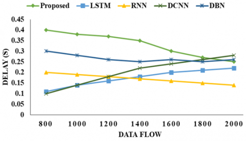
In Table 4 and Figure 4, the characterization shows the Delay flow vs delay. In the analysis of the proposed model, 800 data flows are achieved with the delay at 0.40, 1000 data flows with the delay at 0.38, 1200 data flows with the delay at 0.37, 1400 data flows with the delay at 0.35, 1600 data flows with the delay at 0.30, 1800 data flows with the delay at 0.27, and 2000 data flows with the delay at 0.25, respectively.
Table 4. Delay flow vs delay
|
Data Flow |
800 |
1000 |
1200 |
1400 |
1600 |
1800 |
2000 |
|
Proposed |
0.40 |
0.38 |
0.37 |
0.35 |
0.30 |
0.27 |
0.25 |
|
LSTM |
0.11 |
0.14 |
0.16 |
0.18 |
0.20 |
0.21 |
0.22 |
|
RNN |
0.20 |
0.19 |
0.18 |
0.17 |
0.16 |
0.15 |
0.14 |
|
DCNN |
0.10 |
0.14 |
0.18 |
0.22 |
0.24 |
0.26 |
0.28 |
|
DBN |
0.30 |
0.28 |
0.26 |
0.25 |
0.26 |
0.25 |
0.26 |
Figure 4. Delay analysis
Next, the LSTM model achieves 800 data flows with the delay at 0.11, 1000 data flows with the delay at 0.14, 1200 data flows with the delay at 0.16, 1400 data flows with the delay at 0.18, 1600 data flows with the delay at 0.20, 1800 data flows with the delay at 0.21, and 2000 data flows with the delay at 0.22, respectively.
Following that, the RNN model attains 800 data flows with the delay at 0.20, 1000 data flows with the delay at 0.19, 1200 data flows with the delay at 0.18, 1400 data flows with the delay at 0.17, 1600 data flows with the delay at 0.16, 1800 data flows with the delay at 0.15, and 2000 data flows with the delay at 0.14, respectively.
Then, the DCNN model achieves 800 data flows with the delay at 0.10, 1000 data flows with the delay at 0.14, 1200 data flows with the delay at 0.18, 1400 data flows with the delay at 0.22, 1600 data flows with the delay at 0.24, 1800 data flows with the delay at 0.26, and 2000 data flows with the delay at 0.28, respectively.
Finally, the DBN model attains 800 data flows with the delay at 0.30, 1000 data flows with the delay at 0.28, 1200 data flows with the delay at 0.26, 1400 data flows with the delay at 0.25, 1600 data flows with the delay at 0.26, 1800 data flows with the delay at 0.25, and 2000 data flows with the delay at 0.26, respectively.
In Table 5 and Figure 5, it is demonstrated the Traffic flow vs the average number of collisions. In the analysis of the proposed model, 800 data flows result in the sum of collisions as 2, 1000 data flows result in the sum of collisions as 4, 1200 data flows result in the sum of collisions as 6, 1400 data flows result in the sum of collisions as 8, 1600 data flows result in the sum of collisions as 9, 1800 data flows result in the sum of collisions as 10, and 2000 data flows result in the sum of collisions as 11, respectively.
Table 5. Traffic flow vs average number of collisions
|
Data Flow |
800 |
1000 |
1200 |
1400 |
1600 |
1800 |
2000 |
|
Proposed |
2 |
4 |
6 |
8 |
9 |
10 |
11 |
|
LSTM |
3 |
3 |
4 |
4 |
6 |
6 |
8 |
|
RNN |
1 |
2 |
2 |
2 |
3 |
3 |
5 |
|
DCNN |
1 |
3 |
4 |
5 |
5 |
7 |
7 |
|
DBN |
0 |
1 |
1 |
1 |
2 |
2 |
3 |
Figure 5. Analysis of collisions
Next, the LSTM model achieves 800 data flows with the sum of collisions as 3, 1000 data flows with the sum of collisions as 3, 1200 data flows with the sum of collisions as 4, 1400 data flows with the sum of collisions as 4, 1600 data flows with the sum of collisions as 6, 1800 data flows with the sum of collisions as 6, and 2000 data flows with the sum of collisions as 8, respectively.
Following that, the RNN model attains 800 data flows with the sum of collisions as 1, 1000 data flows with the sum of collisions as 2, 1200 data flows with the sum of collisions as 2, 1400 data flows with the sum of collisions as 2, 1400 data flows with the sum of collisions as 3, 1600 data flows with the sum of collisions as 3, and 1800 data flows with the sum of collisions as 5, respectively.
Then, the DCNN model achieves 800 data flows with the sum of collisions as 1, 1000 data flows with the sum of collisions as 3, 1200 data flows with the sum of collisions as 4, 1400 data flows with the sum of collisions as 5, 1600 data flows with the sum of collisions as 5, 1800 data flows with the sum of collisions as 7, and 2000 data flows with the sum of collisions as 7, respectively.
Finally, the DBN model attains 800 data flows with the sum of collisions as 0, 1000 data flows with the sum of collisions as 1, 1200 data flows with the sum of collisions as 1, 1400 data flows with the sum of collisions as 1, 1600 data flows with the sum of collisions as 2, 1800 data flows with the sum of collisions as 2, and 2000 data flows with the sum of collisions as 3, respectively.
Analyze the learning dynamics of the Q-learning algorithm over the course of training episodes. Plot learning curves to visualize how the agent's performance evolves over time and assess convergence behavior.
Investigate any instances of slow convergence or instability in the learning process. Identify potential causes, such as suboptimal hyperparameters, insufficient exploration, or convergence to local optima, and propose strategies to address these issues.
The optimization and coordination of modern AI task-oriented structures heavily rely on AI-based solutions. As the number of smart devices continues to rise, there is a growing need to develop efficient strategies for managing dispersed co-inference-oriented service optimization issues. In this context, this paper focuses specifically on deep Q-learning, aiming to address the challenge of optimizing total throughput in a three-tier synergistic inference scheme. The main challenge in optimizing total throughput lies in finding a balance among imbalanced resources such as transmission, computation, and caching. Traditional approaches often struggle to effectively allocate resources and coordinate tasks in such heterogeneous environments, leading to suboptimal performance and resource wastage. In this article, we propose a priority-based advancement method and a deep Q-learning-based multicopy reserve allocation procedure to address these challenges. Our approach leverages the consumption of multiple resources after establishing the Lyapunov stability of virtual queues, enabling more efficient utilization of available resources and better coordination of inference tasks across the network. Through empirical evaluations and performance assessments, we demonstrate the viability and superiority of our proposed approach for the distributed co-inference scheme. Our results show a significant throughput increase of 11.3 percent compared to other benchmarks, highlighting the effectiveness of our approach in optimizing resource allocation and improving overall system performance.
Additionally, we aim to investigate the applicability of our approach in various real-world scenarios and diverse domains beyond the scope of our current study. This includes exploring its effectiveness in domains such as edge computing, Internet of Things (IoT) networks, and cloud-based services, where distributed co-inference schemes are prevalent.
[1] Liu, Q., Cheng, L., Jia, A.L., Liu, C. (2021). Deep reinforcement learning for communication flow control in wireless mesh networks. IEEE Network, 35(2): 112-119. https://doi.org/10.1109/MNET.011.2000303
[2] Li, Z., Yu, H., Zhang, G., Dong, S., Xu, C.Z. (2021). Network-wide traffic signal control optimization using a multi-agent deep reinforcement learning. Transportation Research Part C: Emerging Technologies, 125: 103059. https://doi.org/10.1016/j.trc.2021.103059
[3] Alavizadeh, H., Alavizadeh, H., Jang-Jaccard, J. (2022). Deep Q-learning based reinforcement learning approach for network intrusion detection. Computers, 11(3): 41. https://doi.org/10.3390/computers11030041
[4] Baswaraju, S., Maheswari, V.U., Chennam, K.K., Thirumalraj, A., Kantipudi, M.P., Aluvalu, R. (2023). Future food production prediction using AROA based hybrid deep learning model in agri-sector. Human-Centric Intelligent Systems, 3(4): 521-536. https://doi.org/10.1007/s44230-023-00046-y
[5] Macherla, H., Kotapati, G., Sunitha, M.T., Chittipireddy, K.R., Attuluri, B., Vatambeti, R. (2023). Deep learning framework-based chaotic hunger games search optimization algorithm for prediction of air quality index. Ingénierie des Systèmes d’Information, 28(2): 433-441. https://doi.org/10.18280/isi.280219
[6] Wang, G., Hu, J., Li, Z., Li, L. (2021). Harmonious lane changing via deep reinforcement learning. IEEE Transactions on Intelligent Transportation Systems, 23(5): 4642-4650. https://doi.org/10.1109/TITS.2020.3047129
[7] Wang, T., Cao, J., Hussain, A. (2021). Adaptive traffic signal control for large-scale scenario with cooperative group-based multi-agent reinforcement learning. Transportation Research Part C: Emerging Technologies, 125: 103046. https://doi.org/10.1016/j.trc.2021.103046
[8] Rao, M.V., Sreeraman, Y., Mantena, S.V., Gundu, V., Roja, D., Vatambeti, R. (2024). Brinjal crop yield prediction using shuffled shepherd optimization algorithm based ACNN-OBDLSTM model in smart agriculture. Journal of Integrated Science and Technology, 12(1): 710.
[9] Wang, L., Mao, W., Zhao, J., Xu, Y. (2021). DDQP: A double deep Q-learning approach to online fault-tolerant SFC placement. IEEE Transactions on Network and Service Management, 18(1): 118-132. https://doi.org/10.1109/TNSM.2021.3049298
[10] Shi, H., Zhou, Y., Wu, K., Wang, X., Lin, Y., Ran, B. (2021). Connected automated vehicle cooperative control with a deep reinforcement learning approach in a mixed traffic environment. Transportation Research Part C: Emerging Technologies, 133: 103421. https://doi.org/10.1016/j.trc.2021.103421
[11] Xia, D., Wan, J., Xu, P., Tan, J. (2022). Deep reinforcement learning-based QoS optimization for software-defined factory heterogeneous networks. IEEE Transactions on Network and Service Management, 19(4): 4058-4068. https://doi.org/10.1109/TNSM.2022.3208342
[12] Wang, Y., Sarkar, E., Li, W., Maniatakos, M., Jabari, S.E. (2021). Stop-and-go: Exploring backdoor attacks on deep reinforcement learning-based traffic congestion control systems. IEEE Transactions on Information Forensics and Security, 16: 4772-4787. https://doi.org/10.1109/TIFS.2021.3114024
[13] Wei, H., Zheng, G., Gayah, V., Li, Z. (2021). Recent advances in reinforcement learning for traffic signal control: A survey of models and evaluation. ACM SIGKDD Explorations Newsletter, 22(2): 12-18. https://doi.org/10.1145/3447556.3447565
[14] Zhu, H., Gupta, V., Ahuja, S. S., Tian, Y., Zhang, Y., Jin, X. (2021). Network planning with deep reinforcement learning. In Proceedings of the 2021 ACM SIGCOMM 2021 Conference, Virtual Event, USA, pp. 258-271. https://doi.org/10.1145/3452296.3472902
[15] Naderializadeh, N., Sydir, J.J., Simsek, M., Nikopour, H. (2021). Resource management in wireless networks via multi-agent deep reinforcement learning. IEEE Transactions on Wireless Communications, 20(6): 3507-3523. https://doi.org/10.1109/TWC.2021.3051163
[16] Li, Q., Ng, K.K., Simon, C.M., Yiu, C.Y., Lyu, M. (2023). Recognising situation awareness associated with different workloads using EEG and eye-tracking features in air traffic control tasks. Knowledge-Based Systems, 260: 110179. https://doi.org/10.1016/j.knosys.2022.110179
[17] Çelik, Ü., Eren, H. (2023). Classification of manifold learning-based flight fingerprints of UAVs in air traffic. IEEE Transactions on Intelligent Transportation Systems, 24(5): 5229-5238. https://doi.org/10.1109/TITS.2023.3237159
[18] Manimurugan, S., Almutairi, S. (2023). Non-divergent traffic management scheme using classification learning for smart transportation systems. Computers and Electrical Engineering, 106: 108581. https://doi.org/10.1016/j.compeleceng.2023.108581
[19] Sheng, C., Yao, Y., Li, W., Yang, W., Liu, Y. (2023). Unknown attack traffic classification in SCADA network using heuristic clustering technique. IEEE Transactions on Network and Service Management, 20(3): 2625-2638. https://doi.org/10.1109/TNSM.2023.3238402
[20] Alghamdi, A.S., Saeed, A., Kamran, M., Mursi, K.T., Almukadi, W.S. (2023). Vehicle classification using deep feature fusion and genetic algorithms. Electronics, 12(2): 280. https://doi.org/10.3390/electronics12020280
[21] Mane, D., Bidwe, R., Zope, B., Ranjan, N. (2022). Traffic density classification for multiclass vehicles using customized convolutional neural network for smart city. In Communication and Intelligent Systems: Proceedings of ICCIS 2021, New Delhi, India, pp. 1015-1030. https://doi.org/10.1007/978-981-19-2130-8_78
[22] Zhang, C., Dong, M., Ota, K. (2020). Enabling computational intelligence for green Internet of Things: Data-driven adaptation in LPWA networking. IEEE Computational Intelligence Magazine, 15(1): 32-43. https://doi.org/10.1109/MCI.2019.2954642
[23] Davydow, A., Chuprikov, P., Nikolenko, S.I., Kogan, K. (2017). Throughput optimization with latency constraints. In EEE INFOCOM 2017 - IEEE Conference on Computer Communications, Atlanta, GA, USA, pp. 1-9. https://doi.org/10.1109/INFOCOM.2017.8057015
[24] Wu, J., Dong, M., Ota, K., Li, J., Guan, Z. (2017). FCSS: Fog-computing-based content-aware filtering for security services in information-centric social networks. IEEE Transactions on Emerging Topics in computing, 7(4): 553-564. https://doi.org/10.1109/TETC.2017.2747158
[25] Chou, Y.L., Moreira, C., Bruza, P., Ouyang, C., Jorge, J. (2022). Counterfactuals and causability in explainable artificial intelligence: Theory, algorithms, and applications. Information Fusion, 81: 59-83. https://doi.org/10.1016/j.inffus.2021.11.003
[26] Nakhkash, M.R., Gia, T.N., Azimi, I., Anzanpour, A., Rahmani, A.M., Liljeberg, P. (2019). Analysis of performance and energy consumption of wearable devices and mobile gateways in IoT applications. In Proceedings of the International Conference on Omni-Layer Intelligent Systems, Crete, Greece, pp. 68-73. https://doi.org/10.1145/3312614.3312632
[27] Sutton, R.S., Barto, A.G. (2018). Reinforcement Learning: An Introduction. MIT Press, USA.
[28] Mnih, V., Kavukcuoglu, K., Silver, D., et al. (2015). Human-level control through deep reinforcement learning. Nature, 518(7540): 529-533. https://doi.org/10.1038/nature14236
[29] Moerland, T.M., Broekens, J., Plaat, A., Jonker, C.M. (2023). Model-based reinforcement learning: A survey. Foundations and Trends® in Machine Learning, 16(1): 1-118. http://doi.org/10.1561/2200000086
[30] Ladosz, P., Weng, L., Kim, M., Oh, H. (2022). Exploration in deep reinforcement learning: A survey. Information Fusion, 85: 1-22. https://doi.org/10.1016/j.inffus.2022.03.003
[31] Mohan, P., Subramani, N., Alotaibi, Y., Alghamdi, S., Khalaf, O.I., Ulaganathan, S. (2022). Improved metaheuristics-based clustering with multihop routing protocol for underwater wireless sensor networks. Sensors, 22(4): 1618. https://doi.org/10.3390/s22041618
[32] Thirumalraj, A., Asha, V., Kavin, B.P. (2023). An improved hunter-prey optimizer-based DenseNet model for classification of hyper-spectral images. In AI and IoT-Based Technologies for Precision Medicine, pp. 76-96. https://doi.org/10.4018/979-8-3693-0876-9.ch005