Yamama A. Shafeek*![]() | Hazem I. Ali
| Hazem I. Ali![]()
© 2024 The authors. This article is published by IIETA and is licensed under the CC BY 4.0 license (http://creativecommons.org/licenses/by/4.0/).
OPEN ACCESS
The control of systems like: bipedal locomotion robots, space launch vehicle, offshore wind turbines, and active vibration control systems in buildings and bridges, have to ensure, besides stability and accuracy, the system's insensitivity to parameters' uncertainties, unmodeled dynamics, external disturbances, and measurements noise. In such systems analysis and controller design, a triple inverted pendulum can be used as a benchmark to mimic systems characteristics and effect of different sources of uncertainty. μ-synthesis is a robust control method which seeks a controller that minimizes the robust H-infinity performance of the closed-loop system through D-K iteration. The D-K iteration is not guaranteed to converge to a global, or even local minimum. Hence this paper proposes the enhancement of controller design by applying gazelle optimization technique to shape the fictitious output by determining the parameters of the performance weighting matrix. The incorporation of optimization with controller design allows avoiding getting unnecessarily conservative system at the expense of performance. The developed control system is simulated using Matlab R2023b for different scenarios of system uncertainty. The results show that the requirements of robustness and performance can be balanced through the right choice of cost function. The robust performance measure obtained is 0.6432 which leads to good response for both stabilization and tracking in the presence of uncertainty. The results also show that even the baseline μ-synthesis design achieves higher robust stability margin about 2.818, the proposed optimized method stabilizes the system with overshoot been reduced by 67.65% and steady state error reduced by 5.69% without sacrificing robustness.
gazelle optimization technique, μ-synthesis, robust control, structured singular value, triple inverted pendulum, weighting matrix
The applications of triple inverted pendulum system in robotics, biomedicine, aerospace, building and construction fields have raised the need of continuously improving control methods for such systems that handle the inevitable presence of uncertainties. In order to provide control solutions for such system, special control methods should be developed, tested, and improved using suitable benchmark. The triple inverted pendulum system captures the essence of these complex control problems. For instance, balancing the humanoid robot Advanced Step in Innovative Mobility (ASIMO) navigating uneven terrain involves controlling a triple inverted pendulum system. Also, developing a controller for a triple pendulum helps in improving prosthetics or rehabilitation techniques in biomedicine. Furthermore, the system can be used to improve stabilization and guidance of launch vehicles and rockets and improve building stability like skyscrapers that are prone to sway due to wind or seismic activity.
The control of triple inverted pendulum system faces challenges of nonlinearities, under actuation, and system perturbation (parametric uncertainty of moments of inertia and friction coefficients, unmodeled actuator dynamics, external torque disturbance, and noise in potentiometer readings) [1].
Different studies have been made regarding the control of triple inverted pendulum system. The researches [2-6] used adaptive optimal control, fuzzy logic, Linear Quadratic Regulator (LQR), LQR with Genetic Algorithm, fuzzy LQR optimized by Particle Swarm Optimization (PSO), and interval type-2 fuzzy logic control (IT2FLC) with PSO methods but applied it to the linearized model which doesn't show the real nonlinear system response.
Huang et al. [7] applied optimal LQR based on motion vision to stabilize the triple inverted pendulum, Banijamali et al. [8] proposed a model for learning robust locally-linear controllable embedding (RCE) for prediction and planning, Masrom et al. [9] applied IT2FLC based on PSO to control the motion of the triple inverted pendulum. All of these researches focused on noise effect on the system only. While the studies [10-12] considered the disturbance effect only. Gupta et al. [13] derived a robust state feedback control law to overcome nonlinearities, disturbances, and noise hence, didn't consider the effect of unmodeled dynamics of actuators at high frequencies.
Type-1 fuzzy logic, IT2FLC, and adaptive neural fuzzy inference system (ANFIS) PID control strategies were applied to the triple inverted pendulum without testing system's robustness [14-16]. More recently published studies did not investigate the robustness of the proposed control system neither [17-21].
Robust control has been used to stabilize systems with guaranteed performance [22-26]. The control problem must be expressed as a mathematical optimization problem then the controller that solves this optimization problem is then found. These robust techniques can be readily applied to problems involving multivariable systems.
The studies [27, 28] proposed the strategy of using swarm optimization in the robust control design for congestion avoidance in computer networks and blood glucose control in diabetic patients; respectively. The proposed approach opens the doors for the use of optimization in robust control design for different systems.
The literature review concludes that so far, either the control system development focuses on improving system's robustness (which mostly results in conservative system with low performance characteristics) or focuses on improving system's performance for the nominal system (which usually doesn't hold for the perturbed system)
The control objective of this paper is to develop a robust controller for the triple inverted pendulum system that handles all uncertainties with satisfactory performance. To achieve this goal, a μ-synthesis controller is developed enhanced by gazelle optimization of the performance weighting matrix according to a multi-objective cost function that balances robustness and performance requirements through the right selection of each objective's weight.
This paper is organized as the following: Section 2 describes the mathematical model of the triple inverted pendulum system. Section 3 explains the μ-synthesis controller development and the application of gazelle optimization technique to the control system design. The settings of optimization parameters and the resultant performance weighting transfer matrix are given in section 4. Robustness analysis is made in section 5. Different scenarios of uncertainty are simulated and discussed in section 6. Finally, conclusions about controller effectiveness are stated in section 7.
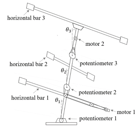
The experimental Furuta triple inverted pendulum consists of three links, two DC motors, two timing belts, three horizontal bar, three potentiometers, and ball bearings as shown in Figure 1 [1].
Figure 1. Triple inverted pendulum [1]
The three arms are connected by ball bearings to reduce friction and to allow smooth rotation in the vertical plane. The DC motors are mounted on the first and third links to supply torque to the two upper hinges through timing belts. A horizontal bar is attached to each arm to make it easier to control by increasing the moment of inertia. The potentiometers are attached to the hinges to measure the angles θ1, θ2, and θ3.
To derive the equations of motion for the system, Lagrange’s equations are used. They relate the partial derivatives of the Lagrangian (difference between the kinetic and potential energies of the system) with respect to the generalized coordinates (angles and velocities) for each pendulum link.
The nonlinear differential equations of motion are:
$M(\theta)\left[\begin{array}{c}\ddot{\theta}_1 \\ \ddot{\theta}_2 \\ \ddot{\theta}_3\end{array}\right]+N_c\left[\begin{array}{l}\dot{\theta}_1 \\ \dot{\theta_2} \\ \dot{\theta_3}\end{array}\right]+\left[\begin{array}{l}q_1 \\ q_2 \\ q_3\end{array}\right]+G\left[\begin{array}{l}t_{m 1} \\ t_{m 2}\end{array}\right]=T\left[\begin{array}{l}d_1 \\ d_2 \\ d_3\end{array}\right]$ (1)
where, θ=[θ1 θ2 θ3)]T is the vector of angles of each arm from the vertical line (as shown in Figure 1), tmj is the control torque of the jth motor, di is the disturbance torque to the ith arm:
$\begin{gathered}M(\theta)= {\left[\begin{array}{ccc}J_1+I_{p 1} & l_1 M_2 \cos \left(\theta_1-\theta_2\right)-I_{p 1} & l_1 M_3 \cos \left(\theta_1-\theta_3\right) \\ l_1 M_2 \cos \left(\theta_1-\theta_2\right)-I_{p 1} & J_2+I_{p 1}+I_{p 2} & l_2 M_3 \cos \left(\theta_2-\theta_3\right)-I_{p 2} \\ l_1 M_3 \cos \left(\theta_1-\theta_3\right) & l_2 M_3 \cos \left(\theta_2-\theta_3\right)-I_{p 2} & J_3+I_{p 2}\end{array}\right]}\end{gathered}$
$N_c=\left[\begin{array}{ccc}C_1+C_2+C_{p 1} & -C_2-C_{p 1} & 0 \\ -C_2-C_{p 1} & C_{p 1}+C_{p 2}+C_2+C_3 & -C_3-C_{p 2} \\ 0 & -C_3-C_{p 2} & C_3+C_{p 2}\end{array}\right]$
$\begin{gathered}q_1=l_1 M_2 \sin \left(\theta_1-\theta_2\right) \dot{\theta}_2^2+l_1 M_3 \sin \left(\theta_1-\theta_3\right) \dot{\theta}_3^2 -M_1 g \sin \left(\theta_1\right)\end{gathered}$
$\begin{gathered}q_2=l_1 M_2 \sin \left(\theta_1-\theta_2\right) \dot{\theta}_1^2+l_2 M_3 \sin \left(\theta_2-\theta_3\right) \dot{\theta}_3^2 -M_2 g \sin \left(\theta_2\right)\end{gathered}$
$\begin{gathered}q_3=l_1 M_3 \sin \left(\theta_1-\theta_3\right)\left(\dot{\theta}_1^2-2 \dot{\theta}_1 \dot{\theta}_3\right)+l_2 M_3 \sin \left(\theta_2-\right. \left.\theta_3\right)\left(\dot{\theta}_2^2-2 \dot{\theta}_2 \dot{\theta}_3\right)-M_3 g \sin \left(\theta_3\right)\end{gathered}$
g is acceleration of gravity,
$G=\left[\begin{array}{cc}K_1 & 0 \\ -K_1 & K_2 \\ 0 & -K_2\end{array}\right], T=\left[\begin{array}{ccc}1 & -1 & 0 \\ 0 & 1 & -1 \\ 0 & 0 & 1\end{array}\right]$
$C_{p i}=C_{p_i^{\prime}}+K_i^2 C_{m i}$,
$I_{p i}=I_{p_i^{\prime}}+K_i^2 I_{m i}, M_1=m_1 h_1+m_2 l_1+m_3 l_1$,
$M_2=m_2 h_2+m_3 l_2, M_3=m_3 h_3$,
$J_1=I_1+m_1 h_1^2+m_2 l_1^2+m_3 l_1^2, J_2=I_2+m_2 h_2^2+m_3 l_2^2$,
$J_3=I_3+m_3 h_3^2$,
where, $l_i$ is the length of the $i^{\text {th }}$ arm, $h_i$ is the distance from the bottom to the center of gravity of the $i^{\text {th }}$ arm, $m_i$ is the mass of the $i^{\text {th }}$ arm, $\alpha_i$ is the gain of the $i^{\text {th }}$ potentiometer, $I_{m j}$ is the moment of inertia of the $j^{\text {th }}$ motor, $C_{p_i^{\prime}}$ is the viscous friction coefficient of the belt-pulley system of the $i^{\text {th }}$ hinge, $I_{p_i^{\prime}}$ is the moment of inertia of the belt-pulley system of the $i^{\text {th }}$ hinge, $K_i$ is the ratio of teeth of belt-pulley system of the $i^{\text {th }}$ hinge, $I_{\dot{j}}$ is the moment of inertia of the $i^{\text {th }}$ arm around the center of gravity, $C_i$ is the viscous friction coefficient of the $i^{\text {th }}$ hinge, $C_{m j i}$ is the viscous friction coefficient of $j^{\text {th }}$ motor. The values of system's parameters are listed in [1].
Since μ-synthesis design involves solving optimization problems with many variables, then employing a linearized model for controller synthesis leads to higher calculations efficiency. Yet, the developed controller is applied to the original nonlinear system. Since the basic requirement in triple inverted pendulum system is its stabilization, small deviation is considered to linearize the model around the operating point (0,0,0) which represents the upright position. However, for large deviations from this point, a nonlinear control approach might be applied. The resulting linearized model equations are:
$M_l\left[\begin{array}{l}\ddot{\theta}_1 \\ \ddot{\theta}_2 \\ \ddot{\theta_3}\end{array}\right]+N_c\left[\begin{array}{l}\dot{\theta}_1 \\ \dot{\theta}_2 \\ \dot{\theta_3}\end{array}\right]+P_l\left[\begin{array}{l}\theta_1 \\ \theta_2 \\ \theta_3\end{array}\right]+G\left[\begin{array}{l}t_{m 1} \\ t_{m 2}\end{array}\right]=T\left[\begin{array}{l}d_1 \\ d_2 \\ d_3\end{array}\right]$ (2)
where, $M_l=\left[\begin{array}{ccc}J_1+I_{p 1} & l_1 M_2-I_{p 1} & l_1 M_3 \\ l_1 M_2-I_{p 1} & J_2+I_{p 1}+I_{p 2} & l_2 M_3-I_{p 2} \\ l_1 M_3 & l_2 M_3-I_{p 2} & J_3+I_{p 2}\end{array}\right]$, and $P_l=\left[\begin{array}{ccc}-M_1 g & 0 & 0 \\ 0 & -M_2 g & 0 \\ 0 & 0 & -M_3 g\end{array}\right]$.
The measured output vector yp is:
$y_p=C_p\left[\begin{array}{l}\theta_1 \\ \theta_2 \\ \theta_3\end{array}\right]$ (3)
where, $C_p=\left[\begin{array}{ccc}\alpha_1 & 0 & 0 \\ -\alpha_2 & \alpha_2 & 0 \\ 0 & -\alpha_3 & \alpha_3\end{array}\right]$ and αi is the gain of the ith potentiometer.
The actuators are modeled as first order transfer functions given by:
$G_{m j}(s)=\frac{K_{m j}}{T_{m j} s+1}$ (4)
The nominal values of the actuator gains Km1 and Km2 are 1.08 and 0.335; respectively, and for time constants Tm1 and Tm2 are 0.005 and 0.002; respectively [1]. To test the effect of the unmodeled dynamics of actuators, that are usually gets excited by high frequencies, on the system, the actuators gains are assumed to be 10% uncertain parameters while the time constants have 20% uncertainty. Input multiplicative uncertainty representation is used to describe the unmodeled actuators dynamics as:
$G_{m j}(s)=\left(1+W_{m j}(s) \delta_{m j}(s)\right) \bar{G}_{m j}(s)$ (5)
where, $W_{m i}(s)$ is the $j_m^{\text {th }}$ actuator uncertainty weight transfer function, $\delta_{m j}(s)$ represents the $j^{\text {th }}$ actuator unmodeled dynamics by uncertain linear time-invariant dynamics with frequency response gain no larger than one, and $\bar{G}_{m j}(s)$ is the nominal transfer function of the $j^{\text {th }}$ motor. By fitting the upper bound of relative error magnitude of the actuator model frequency response to a first order transfer function, the actuator uncertainty weight diagonal transfer matrix $W_m(s)$ is found to be:
$W_m(s)=\left[\begin{array}{cc}\frac{0.3877 s+25.6011}{s+246.3606} & 0 \\ 0 & \frac{0.3803 s+60.8973}{s+599.5829}\end{array}\right]$
The μ-synthesis controller design makes use of the linearized model obtained in section 2 to represent the system in linear fractional transformation form. In the same section, the uncertainty sources of the system were characterized. In this section, the control problem is formulated then solved by D-K iteration. The performance weighting transfer matrix is optimized by Gazelle optimization technique as a part of controller design.
3.1 μ-synthesis controller design
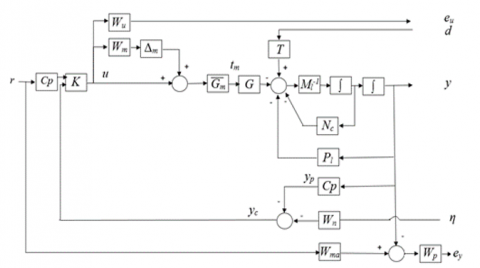
The suggested triple inverted pendulum control system is depicted in Figure 2. In this figure, r represents the reference input vector, u represents the control action vector, d and T represent the input disturbance and its model; respectively, y represents the output vector, h represents the added measurement noise vector, yc represents the measured output vector with noise added, and K represents the two degrees of freedom controller.
Figure 2. Triple inverted pendulum control system
The control signal u(s) represents the input voltage to the DC motors described by:
$u(s)=K(s)\left[\begin{array}{c}y_c(s) \\ C_p r(s)\end{array}\right]$ (6)
The control weighting transfer matrix $W_u(s)$ is set to a $2 \times 2$ diagonal matrix with diagonal elements $10^{-6} \frac{s+1}{0.001 s+1}$. The noise weighting $W_n(s)$ is used to shape the noise spectral density for the potentiometers, it is set to a $3 \times 3$ diagonal matrix with diagonal transfer functions $2 \times 10^{-5} \frac{10 \mathrm{~s}+1}{0.1 \mathrm{~s}+1}$. Since the links have different dynamics speeds (the first link has the slowest dynamics and the third link has the fastest; respectively), the matching model is chosen as [1]:
$W_{m a}(s)=\left[\begin{array}{ccc}\frac{1}{100 s^2+14 s+1} & 0 & 0 \\ 0 & \frac{1}{25 s^2+7 s+1} & 0 \\ 0 & 0 & \frac{1}{9 s^2+4.2 s+1}\end{array}\right]$
such that the dynamics of the three links have an 0.7 damping ratio and different natural frequencies (0.1, 0.2, and 0.333 rad/sec for the first, second, and third link; respectively). In this way, the time constant of the first link is 10 sec, for the second link is 5 sec, and for the third link is 3 sec.
The performance weighting transfer matrix Wp(s) is left to be determined during the optimization of controller design in subsection 3.2.
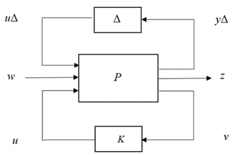
To apply μ-synthesis design, the control system in Figure 2 is transformed to the generalized control configuration shown in Figure 3.
Figure 3. Generalized control configuration
where, $P$ represents the generalized plant model that includes the system model and the interconnection structure between the plant and the controller, and weighting functions. The model uncertainty is pulled out into a block-diagonal matrix $(\Delta), u$ represents the control signals, $w$ represents the weighted exogenous signals $(d, r$, and $\eta), z$ represents the weighted error signals of interest $\left(e_u\right.$ and $\left.e_y\right), v$ represents the input signals to the controller $\left(v_c\right.$ and $\left.C_p r\right), u \Delta$ represents the perturbed input, and $y_{\Delta}$ represents the perturbed output.
The design objective is to find a stabilizing controller $K$, such that for all perturbations satisfying the condition for the upper singular value $\bar{\sigma}$ [29].
$\max _w \bar{\sigma}[\Delta(\mathrm{jw})] \leq 1$ (7)
the closed-loop system is stable and satisfies:
$\left\|F_l\left[F_u(P, \Delta), K\right]\right\|_{\infty} \leq 1$ (8)
where, $\quad F_u(P, \Delta) \triangleq P_{22}+P_{21} \Delta\left(I-P_{11} \Delta\right)^{-1} P_{12} \quad$, $F_l\left(F_u(P, \Delta), K\right) \triangleq F_u(P, \Delta)_{11}+F_u(P, \Delta)_{12} K(I-$ $\left.F_u(P, \Delta)_{22} K\right)^{-1} F_u(P, \Delta)_{21}$, and $\mathrm{P}_{11}, \mathrm{P}_{12}, \mathrm{P}_{21}$, and $\mathrm{P}_{22}$ are the partitions of $P$ in compatibility with the dimensions of $K$ and $\Delta$.
Given any $K$, the structured singular value $\mu_{\Delta}$ can be used to test the robust performance objective by checking the condition:
$\max _w \mu_{\Delta}\left(\left(F_l(P, K)(j w)\right)<1\right.$ (9)
The goal of $\mu$-synthesis is to minimize over all stabilizing controllers $K$, the peak value of $\mu_{\Delta}$ of the closed-loop transfer function $\left(F_L(P, K)\right)$.
$\min _{\substack{K \\ \text { stabilizing }}} \max _w \mu_{\Delta}\left(\left(F_L(P, K)(j w)\right)\right.$ (10)
D-scaling can be used to steer the μ-synthesis algorithm towards solutions that exhibit robust performance across diverse frequency bands by strategically modifying frequency-dependent scales D(jw). In terms of the scaled singular value:
$\min _K\left(\min _{D \in \mathrm{D}}\left\|D F_L(P, K) D^{-1}\right\|_{\infty}\right)$ (11)
where, Ḏ is the set of matrices D which commute with Δ.
The optimization problem (11) is to be solved by D–K iteration approach which combines H-infinity and μ-analysis. In K-step (D(s) is fixed), an H-infinity controller is synthesized for the scaled problem,
$\min _K\left\|D F_L(P, K) D^{-1}\right\|_{\infty}$ (12)
In D-step: (K is fixed), D(jw) that minimizes:
$\bar{\sigma}\left(D(j w) F_L(P, K) D^{-1}(j w)\right)$ (13)
at each frequency is obtained. The magnitude of each element of D (jw) is to be fitted to a stable and minimum phase transfer function D (s). The steps iterate until satisfactory performance is achieved or the H-infinity norm in (12) no longer decreases.
3.2 Incorporating optimization to the controller design
The optimization problems of Eqs. (12) and (13) are convex each, but joint convexity is not guaranteed which may lead to getting trapped by local minimum. To avoid this problem, metaheuristic optimization can be used in determining the gains, numerators' coefficients, and denominators' coefficients of the elements of the performance weighting transfer matrix Wp(s) which is embedded in the generalized plant model P.
Gazelle optimization algorithm is a new nature-inspired population-based metaheuristic algorithm proposed by Agushaka et al. [30]. The optimization procedure of the algorithm comprises of two phases: exploration (searching in large areas with fewer steps) and exploitation (searching effectively in neighborhood areas of promising solutions). Their balance is adjusted dynamically based on the progress of the search. So, this algorithm achieves a good balance between exploration and exploitation due to the way it switches between these phases based on a predator presence.
Both prey and predator are considered search agents. In exploration phase (mimics the chasing of gazelles by predators), the pery solution (major part of population) is updated according to Eq. (14) while the predator solution (minor part of population) is updated according to Eq. (15) [30]:
$\begin{aligned} & \text { gazelle }_{i+1}=\text { gazelle }_i +S \times y \times R \times R_L \times\left(\text { Elite }_i-R_L \times \text { gazelle }_i\right)\end{aligned}$ (14)
$\begin{aligned} & \text { gazelle }_{i+1}=\text { gazelle }_i +S \times y \times C F \times R_B \times\left(\text { Elite }_i\right. \left.-R_L \times \text { gazelle }_i\right) \\ & \end{aligned}$ (15)
where, gazelle $i_{+1}$ and gazelle represent the solution vectors of $^2$ the next and current iteration; respectively, $S$ represents the top speed of gazelle (constant $=88 \mathrm{~km} / \mathrm{h}$ ), y represents the sudden change of direction (constant=+1 or -1 ), $R$ is a vector of uniform random numbers in $[0,1], R_L$ is a vector of random numbers drawn from power law tail distribution to represent the Lévy flight which is a type of random walk characterized by short steps and long jumps, Elite is the vector of the fittest solution, $C F$ is the weight that decreases gradually through iterations according to:
$C F=\left(1-\frac{\text { current iteration index }}{\text { maximum number of iterations }}\right)^{\left(2 \frac{\text { current iteration index }}{\text { maximum number of iterations }}\right)}$ (16)
to determine the transition from Brownian motion to Lévy flight for predators in exploration phase, RB is a vector of random numbers drawn from Gaussian probability distribution with zero mean and unit variance to represent the Brownian motion characterized by uniform and controlled steps.
In exploitation phase (mimics gazelles grazing in the absence of a predator), the population is updated according to [30]:
$\begin{gathered}\text { gazelle }_{i+1}=\text { gazelle }_i+s \times R \times R_B \times\left(\text { Elite }_i-\right. \left.R_B \times \text { gazelle }_i\right)\end{gathered}$ (17)
where, s is drawn from the standard uniform distribution on the open interval (0,1) to represent grazing speed of gazelles.
Gazelles have a 66% chance of surviving each year, which means predators only catch them 34% of the time, the algorithm utilizes the fact that predator success rate is 0.34 to prevent getting stuck in suboptimal solutions.
Figure 4. The proposed controller design steps
Besides having relatively fast convergence, this optimization algorithm has a simpler structure with fewer parameters to adjust compared to other metaheuristic techniques that require careful selection of multiple parameters.
In order to fulfil balancing the robustness and performance of the control system, the cost function is suggested to be comprised of the errors of the three links angles and the robust performance measure $\mu_{\Delta}$ obtained from D-K iteration:
$\begin{gathered}\text { Cost function }=0.2 \times \mathrm{ITAE}_1+0.15 \times \mathrm{ITAE}_2+ 0.15 \times \mathrm{ITAE}_3+0.5 \times \mu_{\Delta}\end{gathered}$ (18)
where,
$\operatorname{ITAE}_i=\int\left|e_i(t)\right| \times t d t$ (19)
and ei represents the error of the ith link. Properly weighting each term in the cost function is very crucial to achieve the desired level of balance between system's robustness and performance. The proposed incorporation of optimization in controller design is illustrated in Figure 4.
The number of search agents used to form the population is 10 initialized randomly within the search space bounded by 0.001 and 20. The maximum number of iterations is 30. The diagonal elements of frequency-dependent 3×3 diagonal performance weighting transfer matrix are to be second order transfer functions; thus the dimension of optimization problem is 21. The resultant performance weighting transfer matrix obtained by optimization is given by:
$\begin{aligned} & W_p(s) =\left[\begin{array}{ccc}0.001 \frac{3.733 s^2+0.001 s+0.001}{0.001 s^2+2.489 s+20} & 0 & 0 \\ 0 & 7.286 \frac{0.195 s^2+6.933 s+1.554}{6.78 s^2+1.411 s+0.057} & 0 \\ 0 & 0 & 2.587 \frac{0.001 s^2+1.913 s+8.45}{7.654 s^2+16.662 s+0.001}\end{array}\right]\end{aligned}$
It is worth to explain that the selected algorithm settings were sufficient for obtaining the performance weighting transfer matrix parameters that achieve minimum value of Eq. (18), increasing the number of iterations wouldn't minimize the cost function any more. The run time of one iteration with 10 search agents takes 20 minutes using 16 GB RAM core i7 SSD laptop, the computational complexity rises from the fact that the D-K iteration is an iterative procedure by its self. Anyway, this is not a problem since the optimization is applied offline during the design process.
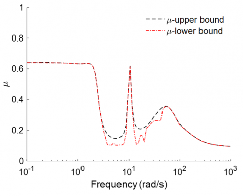
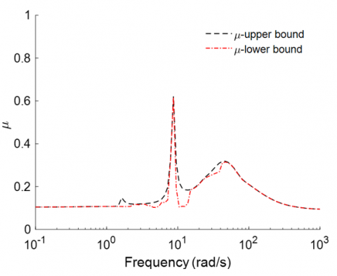
Utilizing the optimal Wp(s) above, the D-K iteration progresses as shown in Table 1. The robust performance measure μ∆ keeps decreasing through the iterations to 0.6432. The structured singular value is usually hard to compute, instead its upper and lower bounds (which are close to each other) are calculated and their peak value must be less than 1 to achieve robust performance. The bounds of robust performance measure of the developed closed loop control system over frequency range [10-1, 103] are shown in Figure 5.
The stability margin is the reciprocal of μ, so the stability margin regarding robust performance falls within the interval [1.5583, 1.5649] which means the tradeoff of model uncertainty and system gain is balanced at a level of 156% of the modeled uncertainty. The critical frequency is 0.1 rad/sec. As for the baseline μ-synthesis control system, the stability margin regarding robust performance falls within the interval [2.4592, 2.4691].
Table 1. D-K iteration progress
|
D-K Iteration |
Peak μ∆ |
D-Order |
|
1 |
2.573 |
28 |
|
2 |
1.246 |
28 |
|
3 |
0.9986 |
24 |
|
4 |
0.8976 |
40 |
|
5 |
0.8548 |
36 |
|
6 |
0.7855 |
36 |
|
7 |
0.7365 |
36 |
|
8 |
0.6997 |
40 |
|
9 |
0.6713 |
48 |
|
10 |
0.6432 |
50 |
Figure 5. Bounds of robust performance
Figure 6 shows the bounds of robust stability of the developed closed loop control system. The stability margin regarding robust stability falls within the interval [1.635, 1.643] so the uncertain system can tolerate up to 164% of the modeled uncertainty. The destabilizing frequency is 10.476 rad/sec and the system is highly robustly stable at frequencies outside the range [6.579, 170.735] rad/sec. As for the baseline μ-synthesis control system, the stability margin regarding robust stability falls within the interval [2.8177, 2.8199].
Figure 6. Bounds of robust stability
The sensitivity of stability margin regarding robust performance and robust stability to variations in each uncertain parameter is given in Table 2. The most influent variation on stability margin is the variation in moment of inertia of the third arm. The least influencers are the variations in hinges' and motors' friction coefficients and moment of inertia of the second arm. Uncertainty in actuators' dynamics has a much greater impact on the system's robust stability than on the system's robust performance.
Table 2. Stability margin sensitivity
|
Parameter |
Sensitivity Regarding Robust Performance |
Sensitivity Regarding Robust Stability |
|
first actuator uncertain dynamics (d1) |
2% |
27% |
|
second actuator uncertain dynamics (d2) |
4% |
56% |
|
viscous friction coefficient of the first hinge (C1) |
2% |
7% |
|
viscous friction coefficient of the second hinge (C2) |
0% |
0% |
|
viscous friction coefficient of the third hinge (C3) |
0% |
0% |
|
viscous friction coefficient of the first motor (Cm1) |
0% |
4% |
|
viscous friction coefficient of the second motor (Cm2) |
0% |
6% |
|
moment of inertia of the first arm around the center of gravity (I1) |
28% |
28% |
|
moment of inertia of the second arm around the center of gravity (I2) |
0% |
1% |
|
moment of inertia of the third arm around the center of gravity (I3) |
65% |
66% |
The developed controller in section 3 has to be validated through simulations of different scenarios of uncertainty. To do so, the stabilization and tracking are considered.
6.1 Case 1 (Stabilization)
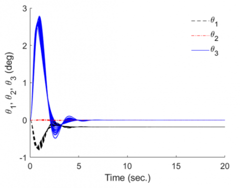
The pendulum is to be stabilized in the upright position in the presence of disturbance and variations in uncertain parameters. The reference, external torque disturbance, and measurement noise vectors are: [0 0 0]T deg, [0.1 0.1 0.1]T N.m, and [0 0 0]T V; respectively. Figure 7 shows the closed-loop system response.
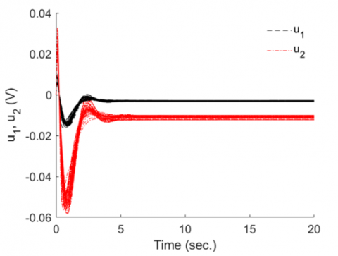
It is shown that 50 samples of the perturbed set have the same behavior which means the system is robust against uncertainty. The second link angle is not affected by applying disturbances, the third link angle overshoots to 2.746 deg then rejects disturbances completely within 5 seconds, the first link settles with unrecognizable steady state error=0.182 deg. As for the baseline μ-synthesis control system, the third link angle overshoots to 8.489 deg then rejects disturbances completely within 10 seconds, the first link settles with unrecognizable steady state error=0.193 deg. The response is obtained by means of the control action shown in Figure 8.
Figure 7. Closed-loop response (case 1)
Figure 8. Control action (case 1)
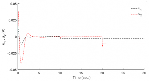
6.2 Case 2 (Stabilization and disturbance rejection)
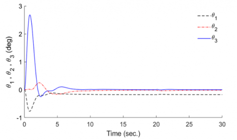
In order to examine the controller behavior to reject disturbance, only one sample of the nonlinear model is simulated through which the disturbances are applied to each link at different times (d1 is applied at t≥0 seconds, d2 at t≥10 seconds, and d3 at t≥20 seconds). The closed loop system response shown in Figure 9 follows the same manner of the 50 samples in Figure 7 with very slight differences. Also, as for the baseline μ-synthesis control system, the third link angle overshoots to 8.54 deg. (much higher than in the proposed control system). Besides that, the disturbance rejection of the baseline μ-synthesis control system in this case is not at the same level of smoothness obtained by the proposed control system.
Figure 9. Closed-loop response (case 2)
The sudden drops in control action at t=0, 10, and 20 seconds shown in Figure 10 aim to counter the effect of disturbances and allow the angles of the links to respond smoothly.
Figure 10. Control action (case 2)
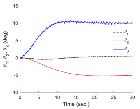
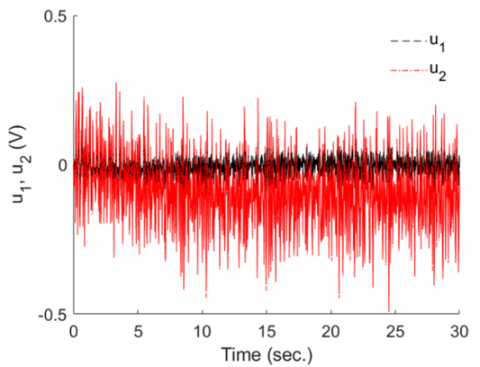
6.3 Case 3 (Tracking of step input)
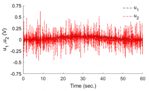
The pendulum is to track the reference [0 -5 10]T deg in the presence of measurement noise [h1 h2 h3]T V where hi is random signal with amplitude range [-0.1, +0.1], and variations in uncertain parameters. The external torque disturbance is [0 0 0]T N.m. the closed-loop system response is shown in Figure 11. All 50 samples respond in the same manner which indicates system's robustness to parametric uncertainties and unmodeled dynamics of actuators. The steady state error of θ1, θ2, and θ3 are 0.23, 0.1, and 0.12 deg; respectively. As for the baseline μ-synthesis control system, the steady state error of θ1, θ2, and θ3 are 0.247, 0.026, and 0.079 deg; respectively. The control action fluctuates as shown in Figure 12 to counter the effect of the applied noise.
Figure 11. Closed-loop response (case 3)
Figure 12. Control action (case 3)
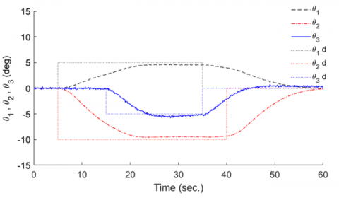
6.4 Case 4 (Tracking of multi-step input)
The pendulum is to track a multi-step reference [θ1d θ2d θ3d]T deg, in the presence of measurement noise $\left[\begin{array}{lll}\eta_1 & \eta_2 & \eta_3\end{array}\right]^{\mathrm{T}} \mathrm{V}$, and disturbance [0 0.1 0]T N.m (applied at t≥25 sec.), where,
$\theta_1 d=\left\{\begin{array}{c}0 \text { deg for } 0 \leq t<5 \\ 5 \text { deg for } 5 \leq t<35 \\ 0 \text { deg for } t \geq 35 \mathrm{sec} .\end{array}\right\}$,
$\theta_2 d=\left\{\begin{array}{c}0 \text { deg for } 0 \leq t<5 \\ -10 \text { deg for } 5 \leq t<40 \\ 0 \text { deg for } t \geq 40 \mathrm{sec} .\end{array}\right\}$, and
$\theta_3 d=\left\{\begin{array}{c}0 \text { deg for } 0 \leq t<15 \\ -5 \text { deg for } 15 \leq t<35 \\ 0 \text { deg for } t \geq 35 \mathrm{sec}\end{array}\right\}$.
Figure 13 shows the tracking of the three links to their corresponding reference signals in spite of disturbance and noise. The third link tracks its reference faster than the first two links. The control action of this case is shown in Figure 14.
Figure 13. Closed-loop response (case 4)
Figure 14. Control action (case 4)
An intuitive insight of the results show that the ability of manipulating the performance weighting function by optimization based on the structured singular value and tracking errors provides the potency of balancing robustness and performance requirements for control systems.
The problem of controlling uncertain nonlinear under actuated triple inverted pendulum system was investigated. A new twist to μ-synthesis robust control design was made by incorporating the optimization in performance weighting determination. The incorporation of gazelle optimization technique allowed to balance the aspects of robustness and performance by including the robust performance measure and output errors in its cost function. The designer can set the weights of the cost function according to his/her control problem to achieve the desired compromise. Although the linearized model around the point (0, 0, 0) was used to develop the controller, the effectiveness of the developed control strategy was tested for both stabilization and tracking problems of the nonlinear system under different scenarios of uncertainty. The developed controller could successfully: manage the nonlinear system uncertainty, reject disturbance, counteract the measurement noise effect, and maintain good performance. Correlating the robustness analysis in section 5 and the results in section 6 shows that the baseline μ-synthesis control system focuses on achieving higher robustness on the expense of system performance, while the proposed controller balances both robustness and performance aspects for the system.
Upon these findings, it is interesting to apply the proposed method to other control systems in future work. A still existing open issue for μ-synthesis controllers is that their design process and computational demands can significantly increase and become challenging to design for very high-order systems. A promising improvement of μ-synthesis controllers design would be made through merging machine learning techniques for uncertainty quantification and controller adaptation by incorporating data from system operation into the control design process.
|
C1 |
viscous friction coefficient of the first hinge, N . m. s |
|
C2 |
viscous friction coefficient of the second hinge, N . m. s |
|
C3 |
viscous friction coefficient of the third hinge, N . m. s |
|
Cm1 |
viscous friction coefficient of the first motor, N . m.s |
|
Cm2 |
viscous friction coefficient of the second motor, N. m. s |
|
$C_{p_1^{\prime}}$ |
viscous friction coefficient of the belt–pulley system of the first hinge, N. m. s |
|
$C_{p_2^{\prime}}$ |
viscous friction coefficient of the belt–pulley system of the second hinge, N. m. s |
|
h1 |
the distance from the bottom to the center of gravity of the first arm, m |
|
h2 |
the distance from the bottom to the center of gravity of the second arm, m |
|
h3 |
the distance from the bottom to the center of gravity of the third arm, m |
|
I1 |
moment of inertia of the first arm around the center of gravity, kg. m2 |
|
I2 |
moment of inertia of the second arm around the center of gravity, kg. m2 |
|
I3 |
moment of inertia of the third arm around the center of gravity, kg. m2 |
|
Im1 |
moment of inertia of the first motor, kg. m2 |
|
Im2 |
moment of inertia of the second motor, kg. m2 |
|
$I_{p_1^{\prime}}$ |
moment of inertia of the belt–pulley system of the first hinge, kg. m2 |
|
$I_{p_2^{\prime}}$ |
moment of inertia of the belt–pulley system of the second hinge, kg. m2 |
|
K1 |
dimentionless ratio of teeth of belt–pulley system of the first hinge |
|
K2 |
dimentionless ratio of teeth of belt–pulley system of the second, hinge |
|
l1 |
length of the first arm, m |
|
l2 |
length of the second arm, m |
|
m1 |
mass of the first arm, kg |
|
m2 |
mass of the second arm, kg |
|
m3 |
mass of the third arm, kg |
|
α1 |
gain of the first potentiometer, V. rad-1 |
|
α2 |
gain of the second potentiometer, V. rad-1 |
|
α3 |
gain of the third potentiometer, V. rad-1 |
|
μ |
dimentionless structured singular value |
[1] Gu, D., Petkov, P.H., Konstantinov, M.M. (2013). Robust control design with MATLAB. United Kingdom: Springer London.
[2] Pang, B., Jiang, Z.P. (2021). Adaptive optimal control of linear periodic systems: An off-policy value iteration approach. IEEE Transactions on Automatic Control, 66(2): 888-894. http://doi.org/10.1109/TAC.2020.2987313
[3] Abdullah, A.I., Alnema, Y.H.S., Thanoon, M.A. (2022). Stabilization of three links inverted pendulum with cart based on genetic LQR approach. Journal Européen des Systèmes Automatisés, 55(1): 125-130. https://doi.org/10.18280/jesa.550113
[4] Abdul Samad, B., Mohamed, M., Anayi, F. (2023). Enhanced the control strategy of a triple link robotic system (robogymnast). IEEE Access, 11: 31997-32005. http://doi.org/10.1109/ACCESS.2023.3262190
[5] Abdul Samad, B., Mohamed, M., Anayi, F. (2023). Motion planning of triple links robotic system. Engineering Proceedings, 31(1): 48. https://doi.org/10.3390/ASEC2022-13774
[6] Masrom, M., Ghani, N., Tokhi, M. (2021). Particle swarm optimization and spiral dynamic algorithm-based interval type-2 fuzzy logic control of triple-link inverted pendulum system: A comparative assessment. Journal of Low Frequency Noise, Vibration and Active Control, 40(1): 367-382. http://doi.org/10.1177/1461348419873780
[7] Huang, X., Wen, F., Wei, Z. (2018). Optimization of triple inverted pendulum control process based on motion vision. EURASIP Journal on Image and Video Processing, 2018(1): 73. http://doi.org/10.1186/s13640-018-0294-6
[8] Banijamali, E., Shu, R., Bui, H., Ghodsi, A. (2018). Robust locally-linear controllable embedding. In International Conference on Artificial Intelligence and Statistics, pp. 1751-1759.
[9] Masrom, M.F., Ghani, N.M., Jamin, N.F., Razali, N.A. A. (2019). Motion control of triple links inverted pendulum on two-wheeled system using interval type-2 fuzzy logic control base on particle swarm optimization. In 2019 9th IEEE International Conference on Control System, Computing and Engineering (ICCSCE), pp. 104-109. http://doi.org/10.1109/ICCSCE47578.2019.9068536
[10] Hussein, M.T. (2018). CAD design and control of triple inverted-pendulums system. The Iraqi Journal for Mechanical and Material Engineering, 18(3): 481-497. http://doi.org/10.32852/iqjfmme.v18i3.183
[11] Masrom, M.F., Ghani, N.M., Jamin, N.F., Razali, N.A.A. (2019). Stabilization control of a two-wheeled triple link inverted pendulum system with disturbance rejection. In Proceedings of the 10th National Technical Seminar on Underwater System Technology 2018: NUSYS'18, pp. 151-159. https://doi.org/10.1007/978-981-13-3708-6_13
[12] Gonzalez Villarreal, O.J., Rossiter, J.A., Tsourdos, A. (2022). An efficient condensing algorithm for fast closed loop dual-mode nonlinear model predictive control. IET Control Theory & Applications, 16(9): 872-888. https://doi.org/10.1049/cth2.12274
[13] Gupta, M.K., Roushan K., Verma, V., Sharma, A. (2021). Robust control based stability analysis and trajectory tracking of triple link robot manipulator. Journal Européen des Systèmes Automatisés, 54(4): 641-647. https://doi.org/10.18280/jesa.540414
[14] Masrom, M.F., Ghani, N.M., Jamin, N.F., Razali, N.A.A. (2018). Control of triple link inverted pendulum on two-wheeled system using IT2FLC. In 2018 IEEE International Conference on Automatic Control and Intelligent Systems (I2CACIS), pp. 29-34. http://doi.org/10.1109/I2CACIS.2018.8603713
[15] Yuvaraja, T., Ramya, K. (2018). Lenient computation in controlling the nonlinear system based on adaptive error optimisation in microgrid. International Journal of Intelligent Machines and Robotics, 1(1): 5-15. http://doi.org/10.1504/IJIMR.2018.090941
[16] Kavirayani, S., Salma, U. (2019). Fuzzy granular computing controls ill-conditioned matrix definitions for triple inverted pendulum. In Soft Computing in Data Analytics: Proceedings of International Conference on SCDA 2018, pp. 533-545. http://doi.org/10.1007/978-981-13-0514-6_52
[17] Sayer, N.A., Kamil, H.G., Al-Moadhen, A.A. (2023). Improving of swing up motion control parameters for a gymnastics robot using the gray wolf algorithm. International Journal of Intelligent Systems and Applications in Engineering, 11(6s): 441-450.
[18] Wu, F., Wang, G., Zhuang, S., Wang, K., Keimer, A., Stoica, I., Bayen, A. (2024). Composing MPC with LQR and neural network for amortized efficiency and stable control. IEEE Transactions on Automation Science and Engineering, 21(2): 2088-2101. http://doi.org/10.1109/TASE.2023.3259428
[19] Han, F., Yi, J. (2023). Cascaded nonlinear control design for highly underactuated balance robots. arXiv preprint arXiv:2309.16805. https://arxiv.org/abs/2309.16805.
[20] Manzl, P., Rogov, O., Gerstmayr, J., Mikkola, A., Orzechowski, G. (2023). Reliability evaluation of reinforcement learning methods for mechanical systems with increasing complexity. Multibody System Dynamics, 1-25. https://doi.org/10.1007/s11044-023-09960-2
[21] Mohamed, M., Abdul Samad, B., Anayi, F., Packianather, M., Yahya, K. (2023). Analysing various control technics for manipulator robotic system (robogymnast). Computers, Materials & Continua, 75(3): 4681-4696. http://doi.org/10.32604/cmc.2023.035312
[22] Mhmood, A.H., Ali, H.I. (2021). Optimal H-infinity PID model reference controller design for roll control of a Tail-Sitter VTOL UAV. Engineering and Technology Journal, 39(4): 552-564. https://doi.org/10.30684/etj.v39i4A.1861
[23] Hassan, M.Y., Ali, H.I., Jassim, H.M. (2020). Hybrid H-infinity fuzzy logic controller design. Journal of Engineering Science and Technology, School of Engineering, Taylor’s University, 15(1): 1-21.
[24] Ali, H.I., Abdulridha, A.J. (2018) H-infinity based full state feedback controller design for human swing leg. Engineering and Technology Journal, 36(3): 350-357. https://doi.org/10.30684/etj.36.3A.15
[25] Mhmood, A.H., Ali, H.I. (2022). Optimal adaptive guaranteed‑cost H‑infinity model reference controller design for nonlinear systems. International Journal of Dynamics and Control, 10(3): 843-856. http://doi.org/10.1007/s40435-021-00846-9
[26] Mhmood, A.H., Ali, H.I. (2021). Optimal H‑infinity integral dynamic state feedback model reference controller design for nonlinear systems. Arabian Journal for Science and Engineering, Springer, 46(10): 10171-10184. https://doi.org/10.1007/s13369-021-05447-4
[27] Qaraawy, S., Ali, H., Mahmood, A. (2012). Particle swarm optimization based robust controller for congestion avoidance in computer networks. In 2012 International Conference on Future Communication Networks, pp. 18-22. http://doi.org/10.1109/ICFCN.2012.6206865
[28] Ali, H., (2014). Design of PSO based robust blood glucose control in diabetic patients. Iraqi Journal of Computers, Communications, Control, and Systems Engineering, 14(1): 1-9.
[29] Skogestad, S., Postlethwaite, I. (2005). Multivariable feedback control: Analysis and design. John Wiley & Sons.
[30] Agushaka, O., Ezugwu, A., Abualigah, L. (2023). Gazelle optimization algorithm: A novel nature-inspired metaheuristic optimizer. Neural Computing and Applications, 35(5): 4099-4131. http://doi.org/10.1007/s00521-022-07854-6