Huthaifa Al-Khazraji*![]() | Rash M. Naji
| Rash M. Naji![]() | Mustafa K. Khashan
| Mustafa K. Khashan![]()
© 2024 The authors. This article is published by IIETA and is licensed under the CC BY 4.0 license (http://creativecommons.org/licenses/by/4.0/).
OPEN ACCESS
An active magnetic bearing (AMB) is a frictionless bearing used in high-speed motors and other electromechanical products. Due to its open loop instability, utilization of controller is essential to stabilize the system. In this paper, a comparative study between sliding mode control (SMC) and back-stepping control (BSC) are presented for AMB systems. These two controller techniques have been applied for various dynamical systems to obtain stable control systems. On the basis of avoiding the chattering in the SMC design, the power rate reaching is introduced in the design of the control action of SMC. In terms of BSC design, Lyapunov-stability theorem is utilized to derive the control low of the controller. A gorilla troops optimization (GTO) has been applied to tune the adjustable parameters of the proposed controllers. According to the computer simulation based on MATLAB software, the results indicate a superior performance and improved in the system response of the SMC as compared to the BSC controller. In addition, the SMC strategy has a good disturbance rejection capability as compared to the BSC strategy.
active magnetic bearing, sliding mode control, back-stepping control, gorilla troops optimization
An active magnetic bearing (AMB) system is a type of mechatronic system that uses controllable electromagnetic force to levitate and support a rotating shaft without any physical contact [1]. Due to the no contact with the rotor, AMB systems offer many advantages over conventional bearings such as reduction of friction, no lubrication, vibration isolation, less heat losses and noise-free operation [2]. Therefore, AMB has been widely used in many industrial applications such as high-speed motors, turbines, wheel energy storage systems, vacuum pumps, etc. [3].
A variation of the conventional and advance control approaches have been proposed to control the AMB system. The primary objective of controlling the AMB system is to stabilize the rotating shaft at the desired position and maintain its stability in the presence of the external disturbances. Due to its simplicity and easy implementation, many authors proposed the classical Proportional-Integral-Derivative (PID) controller for the AMB system including [2, 4]. However, a classical PID controller may have poor control performance. Therefore, Su et al. [5] and Bo et al. [3] combined the PID controller with an intelligence control and proposed Fuzzy-PID controller as an alternative approach to control the AMB system. Besides the classical PID controller, various advance control approaches have been adopted such as fractional PID controller [6], a second-order sliding mode controller (SMC) [1], and Active Disturbance Rejection Controller (ADRC) [7] to improve the efficiency of the AMB system.
The contribution of this paper is to enhance the operation performance of AMB systems. For this purpose, this paper presents a comparative study between two approaches, SMC and back-stepping control (BSC), to improve the performance of position tracking control of the AMB system. SMC and BSC are promising approaches to the robust tracking control problem.
Recently, several of the controller designers are utilized the optimization techniques to attain an optimal performance of the controller [8-10]. The tuning process of the design variables of the control law is formulated as an optimization problem. Meta-heuristic algorithms are one of the well-known and fast growing optimization methods inspired by the behaviors observed in nature. These algorithms have been successfully used to solve a wide range of optimization problems [11-14]. Motivated by powerful of these algorithm and to get the optimal behavior of the proposed controller, this paper is assigned the tuning process to the gorilla troops optimization (GTO) to tune the adjustable parameters of the SMC and BSC controllers.
The remaining of this paper is structured as follows: the mathematical model of the AMB system is introduced in in Section 2. The detail description of designing the SMC and BSC for the AMB system is given in Section 3. The explanation of the GTA is illustrated in Section 4. Simulation outcomes for position tracking control of the AMB system to validate and evaluate the proposed methods are shown in Section 5. Conclusion is summarized in Section 6.
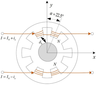
The Schematic of the AMB system that is used in this paper is shown in Figure 1. The ABM system is consisted of a stator core, electromagnetic coil, and rotor [1]. From the control point of view, the model of the single degree of freedom AMB system is represented by the relationship among magnetic force, displacement and current in the Y-direction [7].
Figure 1. Schematic of AMB system [7]
According to the Maxwell’s formula, the electromagnetic attractive force is given by:
$F_m=\frac{\beta^2 A}{\mu_0}$ (1)
where, $\beta, A$ and $\mu_0$ are the magnetic induction intensity between the stator and the rotor, section area and the vacuum permeability respectively. The magnetic induction intensity $\beta$ between the stator and the rotor is given by:
$\beta=\frac{\mu_0 N_c I}{\delta_0}$ (2)
where, $\mathrm{N}_{\mathrm{c}}$, I and $\delta_0$ are number of coil turns, current, and air gap respectively. By substitute Eq. (2) into Eq. (1) obtains:
$\mathrm{F}_{\mathrm{m}}=\mathrm{k} \frac{\mathrm{I}^2}{\delta_0{ }^2}$ (3)
where, $\mathrm{k}=\mu_0 \mathrm{~N}_{\mathrm{c}}{ }^2 \mathrm{~A}$.
In order to stable the suspension of the rotor, the total electromagnetic attractive force $\mathrm{F}_{\mathrm{mt}}$ in the Y-direction is the difference between the upper $\left(\mathrm{F}_{\mathrm{mu}}\right)$ and lower $\left(\mathrm{F}_{\mathrm{ml}}\right)$ of the attraction forces as given [7]:
$\mathrm{F}_{\mathrm{mu}}=\frac{1}{2} \mathrm{k} \frac{\left(\mathrm{I}_0-\mathrm{i}\right)^2}{\left(\delta_0+\mathrm{x} \cos \alpha\right)^2}$ (4)
$\mathrm{F}_{\mathrm{ml}}=\frac{1}{2} \mathrm{k} \frac{\left(\mathrm{I}_0+\mathrm{i}\right)^2}{\left(\delta_0-\mathrm{x} \cos \alpha\right)^2}$ (5)
where, $\alpha$ is the angle between the central axis of the stator and the center line of the electromagnet, i denotes to the control input current and x is the displacement of the rotor.
$\mathrm{F}_{\mathrm{mt}}=2 \mathrm{~F}_{\mathrm{ml}} \cos \alpha-2 \mathrm{~F}_{\mathrm{mu}} \cos \alpha$ (6)
Substitute Eq. (4) and Eq. (5) into Eq. (6) obtains:
$\mathrm{F}_{\mathrm{mt}}=\mathrm{k} \cos \alpha\left(\frac{\left(\mathrm{I}_0+\mathrm{i}\right)^2}{\left(\delta_0-\mathrm{x} \cos \alpha\right)^2}-\frac{\left(\mathrm{I}_0-\mathrm{i}\right)^2}{\left(\delta_0+\mathrm{x} \cos \alpha\right)^2}\right)$ (7)
At the equilibrium point, $\mathrm{x}=0, \mathrm{i}=\mathrm{I}_0$, Taylor expansion is used for Eq. (7) and after omitting the higher order infinitesimal quantities yields:
$\mathrm{F}_{\mathrm{mt}}=\mathrm{k}_{\mathrm{x}} \mathrm{x}+\mathrm{k}_{\mathrm{i}} \mathrm{i}$ (8)
where, $\mathrm{k}_{\mathrm{x}}=4 \mu_0 \mathrm{~N}^2 \mathrm{~A} \cos \alpha \frac{\mathrm{I}_0{ }^2}{\delta_0{ }^2}$ is displacement stiffness coefficient and $\mathrm{k}_{\mathrm{i}}=4 \mu_0 \mathrm{~N}^2 \mathrm{~A} \cos \alpha \frac{\mathrm{I}_0}{\delta_0^2}$ is current stiffness coefficient.
According to the second Newton's law of motion, the rotor motion equation under the action of electromagnetic force is given by:
$\mathrm{m} \ddot{\mathrm{x}}=\mathrm{F}_{\mathrm{mt}}$ (9)
Substitute Eq. (8) into Eq. (9) obtains:
$m \ddot{x}=k_x x+k_i i$ (10)
Let $\mathrm{x}_1$ represents the position $\mathrm{x}, \mathrm{x}_2$ represents the velocity $\dot{\mathrm{x}}$ and $u$ represents the control input $i$. The differential equations of the AMB system are formulated as:
$\dot{\mathrm{x}}_1=\mathrm{x}_2$ (11)
$\dot{\mathrm{x}}_2=\frac{\mathrm{k}_{\mathrm{x}}}{\mathrm{m}} \mathrm{x}_1+\frac{\mathrm{k}_{\mathrm{i}}}{\mathrm{m}} \mathrm{u}$ (12)
There are a various control strategies that can be used for designing control systems. However, SMC and BSC techniques had an important role in the modern control design due to their capabilities to cope with a wide of engineering problems to guarantee the stability of systems [15]. This section presents the details description of establishing the control law of the SMC and BSC for AMB systems.
3.1 Sliding mode control
The SMC is a powerful control strategy that can be used for different control problems such as system with uncertainties and and/or system subject to external disturbances [16]. The basic concept of the SMC approach is to force the system to converge towards a desired surface and then to remain there [17]. In this direction, the design of SMC is consisted of two stages. In the first stage, the sliding surface is defined. Then, in the second stage, the reaching law is introduced.
In the first stage, the sliding surface s is selected as:
$\mathrm{s}=\dot{\mathrm{e}}+\mathrm{a}_{\mathrm{smc}} \mathrm{e}$ (13)
where, e is the tracking position error which is defined as:
$e=x_d-x_1$ (14)
where, $x_d$ is the desired position of the system, $x_1$ is the actual measured position of the system and the coefficient $a_{s m c}\left(a_{s m c}>0\right)$ is a tuning parameters.
Differentiate the error obtains:
$\dot{\mathrm{e}}=\dot{\mathrm{x}}_{\mathrm{d}}-\dot{\mathrm{x}}_1$ (15)
Substitute $\dot{\mathrm{x}}_1$ from Eq. (6) in to Eq. (15) obtains:
$\dot{\mathrm{e}}=\dot{\mathrm{x}}_{\mathrm{d}}-\mathrm{x}_2$ (16)
Differentiate the sliding surface obtains:
$\dot{\mathrm{s}}=\ddot{\mathrm{e}}+\mathrm{a}_{\mathrm{smc}} \dot{\mathrm{e}}=\left(\ddot{\mathrm{x}}_{\mathrm{d}}-\dot{\mathrm{x}}_2\right)+\mathrm{a}_{\mathrm{smc}}\left(\dot{\mathrm{x}}_{\mathrm{d}}-\dot{\mathrm{x}}_1\right)$ (17)
Substitute $\dot{\mathrm{x}}_1$ from Eq. (6) and $\dot{\mathrm{x}}_2$ from Eq. (7) in to Eq. (17) obtains:
$\dot{\mathrm{s}}=\ddot{\mathrm{x}}_{\mathrm{d}}+\mathrm{a}_{\mathrm{smc}} \dot{\mathrm{x}}_{\mathrm{d}}-\frac{\mathrm{k}_{\mathrm{x}}}{\mathrm{m}} \mathrm{x}_1-\frac{\mathrm{k}_{\mathrm{i}}}{\mathrm{m}} \mathrm{u}-\mathrm{a}_{\mathrm{smc}} \mathrm{x}_2$ (18)
As mention above, the second stage of the SMC is to keep the system sliding on surface by using the reaching law. On the basis of avoiding the chattering in the SMC design, the power rate is introduced as a reaching law [18]. The power rate reaching law is given by the study [19]:
$\dot{\mathrm{s}}=-\mathrm{k}_{\mathrm{smc}}|\mathrm{s}|^{\gamma_{\mathrm{smc}}} \operatorname{sgn}(\mathrm{s})$ (19)
where, the coefficient $\mathrm{k}_{\mathrm{smc}}\left(\mathrm{k}_{\mathrm{smc}}>0\right)$ is a tuning parameters, the power rate $\gamma_{s m c}$ is an adjustable parameters between $[0,1]$ and the operator sgn is the Sign function. The final stage of designing the SMC is to keep the system is sliding on surface by determining the control law $u$ that ensures the s in Eq. (18) is equal to the $\dot{s}$ in Eq. (19) as given:
$\begin{aligned} & \ddot{x}_d+a_{s m c} \dot{x}_d-\frac{k_x}{m} x_1-\frac{k_i}{m} u-a_{s m c} x_2 =-\mathrm{k}_{\mathrm{smc}}|\mathrm{s}|^{\gamma_{\mathrm{smc}}} \operatorname{sgn}(\mathrm{s}) \\ & \end{aligned}$ (20)
Rearrange Eq. (20), the control action of the SMC is defined by:
$\begin{aligned} & \mathrm{u}=\frac{\mathrm{m}}{\mathrm{k}_{\mathrm{i}}}\left(\ddot{\mathrm{x}}_{\mathrm{d}}+\mathrm{a}_{\mathrm{smc}} \dot{x}_{\mathrm{d}}+\mathrm{k}_{\mathrm{smc}}|\mathrm{s}|^{\gamma_{\mathrm{smc}}} \operatorname{sgn}(\mathrm{s})-\mathrm{a}_{\mathrm{smc}} \mathrm{x}_2\right. \left.-\frac{\mathrm{k}_{\mathrm{x}}}{\mathrm{m}} \mathrm{x}_1\right) \\ & \end{aligned}$ (21)
3.2 Back-stepping control
BSC is a systematic recursive feedback control design method. Lyapunov function is employed in the design to select control law that guarantees the stability the closed loop system [20]. The design procedure of BSC is explained as follows:
The state $x_2$ of the system is selected as the virtual control $v$. Then, let $e_1$ is defined as the error between the desired position of the system $x_d$ and the actual measured position of the system $\mathrm{x}_1$.
$\mathrm{e}_1=\mathrm{x}_{\mathrm{d}}-\mathrm{x}_1$ (22)
Differentiate of $\mathrm{e}_1$ obtains:
$\dot{\mathrm{e}}_1=\dot{\mathrm{x}}_{\mathrm{d}}-\mathrm{x}_2$ (23)
Choose first Lyapunov function as:
$\mathrm{V}_1=\frac{1}{2} \mathrm{e}_1{ }^2$ (24)
Take the derivative of $V_1$:
$\dot{\mathrm{V}}_1=\mathrm{e}_1 \dot{\mathrm{e}}_1=\mathrm{e}_1\left(\dot{\mathrm{x}}_{\mathrm{d}}-\mathrm{x}_2\right)$ (25)
Substitute v into Eq. (25) as a virtual control for x2 gives:
$\dot{\mathrm{V}}_1=\mathrm{e}_1\left(\dot{\mathrm{x}}_{\mathrm{d}}-\mathrm{v}\right)$ (26)
The virtual control v is selected as:
$\mathrm{v}=\lambda_{\mathrm{bsc}} \mathrm{e}_1+\dot{\mathrm{x}}_{\mathrm{d}}$ (27)
where, the coefficient $\lambda_{\text {smc }}\left(\lambda_{\text {smc }}>0\right)$ is a tuning parameters.
Substitute Eq. (27) into (26), $\dot{\mathrm{V}}_1$ becomes:
$\dot{\mathrm{V}}_1=-\lambda_{\mathrm{hsc}} \mathrm{e}_1^2$ (28)
Eq. (28) ensures that $e_1$ decay exponentially to the zero.
The next step in the design is to define $e_2$ as the error between the virtual control v and the state $x_2$.
$\mathrm{e}_2=\mathrm{x}_2-\mathrm{v}$ (29)
Substitute v as given in Eq. (27) in Eq. (29) obtains:
$\mathrm{e}_2=\mathrm{x}_2-\lambda_{\mathrm{bsc}} \mathrm{e}_1-\dot{\mathrm{x}}_{\mathrm{d}}$ (30)
Rearrange Eq. (30) to obtain $x_2$:
$\mathrm{x}_2=\mathrm{e}_2+\lambda_{\mathrm{bsc}} \mathrm{e}_1+\dot{\mathrm{x}}_{\mathrm{d}}$ (31)
Substitute $x_2$ as given in Eq. (31) into Eq. (6) gives:
$\dot{\mathrm{x}}_1=\mathrm{e}_2+\lambda_{\mathrm{bsc}} \mathrm{e}_1+\dot{\mathrm{x}}_{\mathrm{d}}$ (32)
Take the derivative of $e_2$:
$\dot{\mathrm{e}}_2=\dot{\mathrm{x}}_2-\lambda_{\mathrm{bsc}} \dot{\mathrm{e}}_1-\ddot{\mathrm{x}}_{\mathrm{d}}$ (33)
Choose total Lyapunov function as:
$\mathrm{V}=\frac{1}{2} \mathrm{e}_1{ }^2+\frac{1}{2} \mathrm{e}_2{ }^2$ (34)
Take the derivative of V:
$\dot{\mathrm{V}}=\mathrm{e}_1 \dot{\mathrm{e}}_1+\mathrm{e}_2 \dot{\mathrm{e}}_2$ (35)
Substitute $\dot{\mathrm{e}}_1$ as given in Eq. (23) and $\dot{\mathrm{e}}_2$ as given in (33) into Eq. (35) gives:
$\dot{\mathrm{V}}=\mathrm{e}_1\left(\dot{\mathrm{x}}_{\mathrm{d}}-\mathrm{x}_2\right)+\mathrm{e}_2\left(\dot{\mathrm{x}}_2-\lambda_{\mathrm{bsc}} \dot{\mathrm{e}}_1-\ddot{\mathrm{x}}_{\mathrm{d}}\right)$ (36)
Rearrange Eq. (36) gives:
$\begin{aligned} & \dot{\mathrm{V}}=-\lambda_{\mathrm{bsc}} \mathrm{e}_1{ }^2+\mathrm{e}_2\left(\left(\lambda_{\mathrm{bsc}}{ }^2-1\right) \mathrm{e}_1+\lambda_{\mathrm{bsc}} \mathrm{e}_2+\dot{\mathrm{x}}_2\right. \left.-\ddot{\mathrm{x}}_{\mathrm{d}}\right) & \end{aligned}$ (37)
Substitute $\dot{\mathrm{x}}_2$ as given in Eq. (7) into Eq. (37) gives:
$\begin{aligned} \dot{\mathrm{V}}=-\lambda_{\mathrm{bsc}} \mathrm{e}_1{ }^2+ & \mathrm{e}_2\left(\left(\lambda_{\mathrm{bsc}}{ }^2-1\right) \mathrm{e}_1+\lambda_{\mathrm{bsc}} \mathrm{e}_2\right. \left.+\left(\frac{\mathrm{k}_{\mathrm{x}}}{\mathrm{m}} \mathrm{x}_1+\frac{\mathrm{k}_{\mathrm{i}}}{\mathrm{m}} \mathrm{u}\right)-\ddot{\mathrm{x}}_{\mathrm{d}}\right)\end{aligned}$ (38)
The terms $-\lambda_{\text {bsc }} \mathrm{e}_1^2$ in Eq. (38) ensures that $\mathrm{e}_1$ decay exponentially to the zero. However, to ensure that $e_2$ is decay exponentially to the zero, the term $\left(\left(\lambda_{b s c}{ }^2-1\right) \mathrm{e}_1+\lambda_{\mathrm{bsc}} \mathrm{e}_2+\right.$ $\left.\left(\frac{k_x}{m} x_1+\frac{k_i}{m} u\right)-\ddot{x}_d\right)$ in Eq. (38) need to be $-\gamma_{b s c} e_2{ }^2$ in order to ensure that $\mathrm{e}_1$ decay exponentially to the zero, where $\gamma_{\mathrm{bsc}}$ $\left(\gamma_{\mathrm{smc}}>0\right)$ is a is a tuning parameters. Based on that, the control law of the SMC can be obtained as follows:
$\mathrm{u}=\left(\frac{\mathrm{m}}{\mathrm{k}_{\mathrm{i}}}\right)\left(\left(-\gamma_{\mathrm{bsc}}-\lambda_{\mathrm{bsc}}\right) \mathrm{e}_2-\left(\lambda_{\mathrm{bsc}}{ }^2-1\right) \mathrm{e}_1+\ddot{\mathrm{x}}_{\mathrm{d}}-\frac{\mathrm{k}_{\mathrm{x}}}{\mathrm{m}} \mathrm{x}_1\right)$ (39)
Substitute u as given in Eq. (39) into Eq. (38) gives:
$\dot{\mathrm{V}}=-\lambda_{\mathrm{hsc}} \mathrm{e}_1{ }^2-\gamma_{\mathrm{hsc}} \mathrm{e}_2{ }^2$ (40)
Eq. (40) guaranteed stability of the system and $e_1$ and $\mathrm{e}_2$ will converge to zero as $\mathrm{t} \rightarrow \infty$.
The GTO is an intelligence algorithm established by Abdollahzadeh et al. [21] in 2021. The method is stimulated by the lifestyle of silverback gorillas, such as migration to known places, discovered new places to live in, and competing with gorillas for females [22]. According the silverback gorilla lifestyle, Abdollahzadeh et al. [21] developed an optimization algorithm consists of five equations. The steps to implement the algorithm are given by the pseudo-code in Algorithm 1 below. There out of the five equations of the GTO are used by gorilla to explore new places, visit well-known places, and/or move to other gorilla. In the context of the optimization algorithm, the aim of these there equations is to enhance the exploration process of the search space of the optimization problem. To balance between these three ways of exploration, it is considered that there is a probability which is chosen randomly to select among them. This can be achieved by the following equation:
$\begin{aligned} & \text { GX }(\text { itr }+1) & =\left\{\begin{array}{c}\text { LB }+r_1(U B-L B), \text { rand }<p_1 \\ \text { GR(itr })\left(r_2-k_1\right)+k_2 k_3, \text { rand } \geq 0.5 \\ \text { GX(itr }) -\mathrm{k}_2\binom{\mathrm{k}_2(\mathrm{GX}(\mathrm{itr})-\mathrm{GR}(\mathrm{itr}))}{+\mathrm{r}_3(\mathrm{GX}(\mathrm{itr})-\mathrm{GR}(\mathrm{itr}))}, \text { rand }<0.5\end{array}\right.\end{aligned}$ (41)
where, LB, UB, itr, GX(itr), GR(itr), GX(itr + 1) are lower bound, upper bound, iteration index, current solution, position selected randomly, and new solution respectively. $r_1, r_2, r_3$ are random value between [0, 1]. $\mathrm{p}_1$ is a coefficient defined by the user between [0,1]. The determination of the coefficients $\mathrm{k}_1, \mathrm{k}_2$ and $\mathrm{k}_3$ is given by:
$\mathrm{k}_1=\mathrm{k}_4\left(1-\frac{\mathrm{itr}}{\mathrm{T}_{\max }}\right)$ (42)
$\mathrm{k}_2=\mathrm{k}_1 \mathrm{k}_5$ (43)
$\mathrm{k}_3=\mathrm{k}_6 \mathrm{GX}(\mathrm{itr})$ (44)
$\mathrm{k}_4=\cos \left(2 \mathrm{r}_4\right)+1$ (45)
where, $\mathrm{T}_{\max }$ is the maximum iteration, $\mathrm{r}_4$ is a random value ranges between $[0,1] . \mathrm{k}_5$ is a random value ranges between $[-1,1] . \mathrm{k}_6$ is a random value ranges between $\left[-\mathrm{k}_1, \mathrm{k}_1\right]$.
|
Algorithm1: GTO's Pseudo-Code |
|
1. Input Objective function, Population size (N), Number of iteration (Tmax), parameter p1, p2 and p3 2. Initialization Initialize population N Evaluate objective function 3. Loop: while (itr < Tmax) Update k1, k2, k3 For each Gorilla Update the location Gorilla using Eq. (41) End for Perform greedy selection and update Gsliverback For each Gorilla If |k1| ≥ p2 Update k7 Update the location Gorilla using Eq. (46) Else Update k8 and k9 Update the location Gorilla using Eq. (47) End if End for Perform greedy selection and update Gsliverback itr = itr + 1 End while 4. Print the Optimal Solution |
In the context of exploitation search, the GTO describe this stage by using two equations including the competition for mates and following the silverback. According to the coefficients $\mathrm{k}_1$, the gorillas are either competition for mates or follow the silverback. For example, if $\mathrm{k}_1 \geq \mathrm{p}_2$, gorillas follow the silverback based on Eq. (46), however, if $\mathrm{k}_1<\mathrm{p}_2$, gorillas compete for mate based on Eq. (47), where $\mathrm{p}_2$ is determined by the user [21].
$\begin{aligned} \mathrm{GX}(\mathrm{itr}+1)= & \mathrm{GX}(\mathrm{itr}) +\mathrm{k}_1 \mathrm{k}_7\left(\mathrm{GX}(\mathrm{itr})-\mathrm{G}_{\text {sliverback }}\right)\end{aligned}$ (46)
$\begin{aligned} \text { GX }(\mathrm{itr}+1)= & \mathrm{G}_{\text {sliverback }} -\mathrm{k}_9 \mathrm{k}_8\left(\mathrm{G}_{\text {sliverback }}-\mathrm{GX}(\mathrm{itr})\right)\end{aligned}$ (47)
Coefficients $\mathrm{k}_7, \mathrm{k}_8$, and $\mathrm{k}_9$ are obtained as follows [21]:
$\mathrm{k}_7=\left(\left|\frac{1}{\mathrm{~N}} \sum_{\mathrm{j}=1}^{\mathrm{N}} \mathrm{GX}_{\mathrm{i}}(\mathrm{itr})\right|^{\mathrm{g}}\right)^{\frac{1}{\mathrm{~g}}}$ (48)
$g=2^{k_2}$ (49)
$\mathrm{k}_8=\mathrm{p}_3 \mathrm{k}_{10}$ (50)
$\mathrm{k}_9=2 \mathrm{r}_5-1$ (51)
$\mathrm{k}_{10}=\left\{\begin{array}{l}\mathrm{rn}_1, \text { rand } \geq 0.5 \\ \mathrm{rn}_2, \text { rand }<0.5\end{array}\right.$ (52)
where, $\mathrm{N}$ is the size of the population, $\mathrm{p}_3$ is a coefficient defined by the user. $r_5$ is a random value ranges between $[0,1]$. $\mathrm{rn}_1$ is random value ranges between $[0, \mathrm{~N}] . \mathrm{rn}_2$ is a random value.
In order to evaluate the effectiveness of the proposed control strategy, this section presents a simulation study of controlling the AMB system. Using Matlab software, the proposed controlled models for the AMB system have been simulated. The differential equations of the AMB system that is provided by Eq. (6) and Eq. (7) are used to simulate the system dynamics. The parameters of the controlled system are listed in Table 1 [3]. The initial position of the rotor of the AMB system was set to -0.03 m, and the desired rotor position was 0 mm.
Table 1. Parameters of AMB system
|
Parameters |
Value |
|
Current stiffness $\left(k_i\right)$ |
$184.3 \mathrm{~N} / \mathrm{A}$ |
|
Displacement stiffness $\left(k_x\right)$ |
$1.536 \times 10^6 \mathrm{~N} / \mathrm{m}$ |
The GTO is used to fine-tune the adjusted parameters ($\mathrm{a}_{\mathrm{smc}}, \mathrm{k}_{\mathrm{smc}}$, and $\gamma_{\mathrm{smc}}$) of the SMC's control law that is provided in Eq. (21) and the adjusted parameters ($\lambda_{\mathrm{bsc}}$ and $\gamma_{\mathrm{bsc}}$) of the BSC's control action that is provided in Eq. (39) based on the Integral Time of Absolute Errors (ITAE) as given in Eq. (53) [23, 24].
ITAE $=\int_{\mathrm{tt}=0}^{\mathrm{t}=\mathrm{t}_{\text {sim }}} \mathrm{tt}|\mathrm{e}(\mathrm{t})| \mathrm{dt}$ (53)
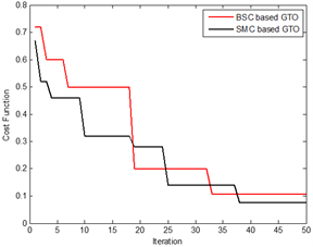
where, $\mathrm{t}_{\mathrm{sim}}$ refers the total simulation time. The tuning variables of the GTO are selected as given in Table 2. The convergence of the GTO algorithm to find the adjusted design variables of the SMC and BSC is illustrated in Figure 2. The values of the adjusted parameters of the SMC and BSC are reported in Table 3.
Table 2. GTO's parameters
|
Parameters |
Value |
|
Population Size (N) |
25 |
|
Number of Iterations ($\mathrm{T}_{\max }$) |
50 |
|
$\mathrm{p}_1$ |
0.03 |
|
$\mathrm{p}_1$ |
3 |
|
$\mathrm{p}_3$ |
0.8 |
Figure 2. Convergence of GTO for the two controllers
Table 3. Optimal controller's design
|
Controller |
Parameters |
Value |
|
SMC |
$\mathrm{k}_{\mathrm{smc}}$ |
10 |
|
$\mathrm{a}_{\mathrm{smc}}$ |
20 |
|
|
$\gamma_{\text {smc }}$ |
0.7 |
|
|
BSC |
$\lambda_{\mathrm{bsc}}$ |
12 |
|
$\gamma_{\mathrm{bsc}}$ |
15 |
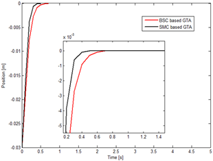
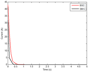
Figure 3 depicts the responses of AMB system to step input. The corresponding control signals due to proposed controllers are illustrated in Figure 4. By comparing the two control approaches (SMC and BSC) as shown in Figure 3 and Table 4, it can be observed that the two controllers are effectively able to control the AMB system with zero overshoot and zero error steady state. The results also show that the SMC has a faster tracking response to the desired output than the BSC. Moreover, the SMC improves the ITAE index by 29.9% where the ITAE index is reduced from 0.107 for the BSC to 0.075 for the SMC. Besides, Figure 4 shows that there is no chattering in the control law for both controllers.
Figure 3. AMB system's position response
Table 4. System's performances
|
Controller |
Settling Times (s) |
Error Steady State (Rad) |
Maximum Overshoot (%) |
ITAE |
|
SMC |
0.3 |
0 |
0 |
0.075 |
|
BSC |
0.45 |
0 |
0 |
0.107 |
Figure 4. Control signals of the proposed controllers
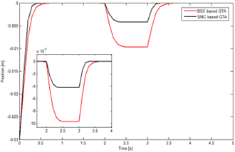
The performance of the two controllers is evaluated under the presence of external disturbance. After two second, an outside force disturbance has been added to each controlled system. Figure 5 shows the performance of the two controlled systems for tracking the desired output with disturbance. The time response specifications of each system are assessed in terms of recovery time and undershoot. These specifications are reported in Table 5.
It is clear from the Figure 5 and Table 5 that the system is recovery from the disturbance to the desired position and remained stable for both controller structures. However, The SMC had 13% undershoot and its recovery time was 1s, which is better when compared with the 30% undershoot and 1.5s recovery time of the BSC. Furthermore, the SMC improves the ITAE index by 57.43% where the value of the ITAE index is reduced from 2.777 in the case of BSC to 1.182 in the case of SMC.
Table 5. System's performance under disturbance
|
Controller |
Recovery Time (s) |
Error Steady State (Rad) |
Maximum Undershoot (%) |
ITAE |
|
SMC |
1 |
0 |
13% |
1.182 |
|
BSC |
1.5 |
0 |
30% |
2.777 |
Figure 5. AMB system's position response under disturbance
Under these two evaluations between the SMC and BSC, it can be revealed that the performance SMC to control the AMB system was superior to BSC in terms of reduce the settling/recover time, overshoot/undershoot and the ITAE.
To address the problem of controlling AMB system, a comparative study of designing SMC and BSC is presented in this paper. In order to prevent chattering phenomena in the SMC, the power rate reaching is incorporated into the SMC control law design. Besides, the Lyapunov stability theorem is used in BSC design to determine the controller's control low. GTO is utilized to fine-tune the adjusted design parameters of the SMC and BSC using the ITAE index. The results show the effectiveness and robustness of the SMC method to handle the tracking control problem and reduce external disturbances in comparison with the BSC. The results data indicate that the SMC enhance the ITAE index by 29.9% under normal operation whereas this enhancement increased to 57.43% when the system is subjected to an external disturbance.
This work can be extended by including different optimization algorithms to tune the design parameters of SMC and BSC such as heap-based optimization [25]. Besides, alternative controller can be adopted for such as adaptive control [10] further improvement.
|
ADRC |
Active disturbance rejection controller |
|
AMB |
Active magnetic bearing |
|
BSC |
Back-stepping control |
|
GTO |
Gorilla troops optimization |
|
PID |
Proportional-Integral-Derivative |
|
SMC |
Sliding mode control |
|
Subscripts |
|
|
A |
Section area |
|
$\mathrm{a}_{\mathrm{smc}}$ |
Tuning parameters $>0$ |
|
$e(t)$ |
Error between the measured output $\mathrm{x}_1(\mathrm{t})$ and the desired output $\mathrm{x}_{\mathrm{d}}(\mathrm{t})$ |
|
$\dot{\mathrm{e}}(\mathrm{t})$ |
First derivative of $\mathrm{e}(\mathrm{t})$ |
|
$\mathrm{F}_{\mathrm{m}}$ |
Electromagnetic attractive force |
|
$\mathrm{F}_{\mathrm{mt}}$ |
Total electromagnetic attractive force |
|
g |
Acceleration of gravity |
|
gn |
Coefficients |
|
$\mathrm{G}_{\text {sliverback }}$ |
Best solution |
|
GR(itr) |
Solution selected randomly |
|
GX(itr) |
Current solution |
|
GX (itr + 1) |
New solution |
|
i |
Index for population |
|
itr |
Index for iteration |
|
$\begin{aligned} & \mathrm{k}_1, \mathrm{k}_2, \mathrm{k}_3, \mathrm{k}_4, \mathrm{k}_7, \mathrm{k}_8, \mathrm{k}_9\end{aligned}$ |
Coefficients |
|
$\mathrm{k}_5$ |
Random number between [-1,1] |
|
$\mathrm{k}_6$ |
Random number between $\left[-\mathrm{k}_1, \mathrm{k}_1\right]$ |
|
$\mathrm{k}_i$ |
Current stiffness |
|
$\mathrm{k}_{smc}$ |
Adjusted parameter $>0$ |
|
$\mathrm{k}_x$ |
Displacement stiffness |
|
N |
Population size |
|
Nc |
Coil turns |
|
$\mathrm{p}_1, \mathrm{p}_2, \mathrm{p}_3$ |
Coefficients determined by the user between [0,1] |
|
$\mathrm{r}_1, \mathrm{r}_2, \mathrm{r}_3, \mathrm{r}_4, \mathrm{r}_5$ |
Random number between [0,1] |
|
$\mathrm{rn}_1$ |
Random number between [0,N] |
|
$\mathrm{rn}_2$ |
Random number |
|
$\mathrm{s}(\mathrm{t})$ |
Sliding surface |
|
$\dot{\mathrm{s}}(\mathrm{t})$ |
First derivative of s(t) |
|
sgn |
Sign function |
|
t |
Time |
|
tsim |
Total simulation time |
|
Tmax |
Maximum iteration |
|
u(t) |
Control law |
|
$\mathrm{x}_1(\mathrm{t})$ |
Position |
|
$\dot{\mathrm{x}}_1(\mathrm{t})$ |
First derivative of $\mathrm{x}_1(\mathrm{t})$ |
|
$\mathrm{x}_2(\mathrm{t})$ |
Velocity |
|
$\dot{\mathrm{x}}_2(\mathrm{t})$ |
First derivative of $\mathrm{x}_2(\mathrm{t})$ |
|
$x_d(t)$ |
Desired output |
|
$\dot{x}_d(t)$ |
First derivative of $\mathrm{x}_d(\mathrm{t})$ |
|
$\ddot{\mathrm{x}}_{\mathrm{d}}(\mathrm{t})$ |
Second Derivative of $\mathrm{x}_d(\mathrm{t})$ |
|
Greek symbols |
|
|
$\alpha$ |
Angle between the central axis of the stator and the center line of the electromagnet |
|
$\beta$ |
Magnetic induction intensity between the stator and the rotor |
|
$\delta_0$ |
Air gap |
|
$\mu_0$ |
Vacuum permeability |
|
$\lambda_{\text {bsc }}$ |
Tuning parameters for SMC |
|
$\gamma_{\mathrm{smc}}$ |
Tuning parameters for SMC |
|
$\gamma_{\mathrm{bmc}}$ |
Tuning parameters for BSC |
[1] Wang, X., Zhang, Y., Gao, P. (2020). Design and analysis of second-order sliding mode controller for active magnetic bearing. Energies, 13(22): 5965. https://doi.org/10.3390/en13225965
[2] Psonis, T.K., Nikolakopoulos, P.G., Mitronikas, E. (2015). Design of a PID controller for a linearized magnetic bearing. International Journal of Rotating Machinery, 2015: 656749. http://dx.doi.org/10.1155/2015/656749
[3] Bo, W., Haipeng, G., Hao, L., Wei, Z. (2021). Particle swarm optimization-based fuzzy PID controller for stable control of active magnetic bearing system. In Journal of Physics, 1888(1): 012022 https://doi.org/10.1088/1742-6596/1888/1/012022
[4] Gupta, S., Laldingliana, J., Debnath, S., Biswas, P.K. (2018). Closed loop control of active magnetic bearing using PID controller. In 2018 International Conference on Computing, Power and Communication Technologies (GUCON), Greater Noida, India, pp. 686-690. https://doi.org/10.1109/GUCON.2018.8675123
[5] Su, Y., Li, X., Zhou, Z., Chen, Y., Zhang, D. (2006). Fuzzy-immune PID control for AMB systems. Wuhan University Journal of Natural Sciences, 11(3): 637-641. https://doi.org/10.1007/BF02836680
[6] Chang, L.Y., Chen, H.C. (2009). Tuning of fractional PID controllers using adaptive genetic algorithm for active magnetic bearing system. WSEAS Transactions on systems, 8(1): 158-167.
[7] Yu, T., Zhang, Z., Li, Y., Zhao, W., Zhang, J. (2023). Improved active disturbance rejection controller for rotor system of magnetic levitation turbomachinery. Electronic Research Archive, 31(3): 1570-1586. https://doi.org/10.3934/era.2023080
[8] Yacef, F., Bouhali, O., Hamerlain, M., Rezoug, A. (2013). PSO optimization of Integral backstepping controller for quadrotor attitude stabilization. In 3rd International Conference on Systems and Control, Algiers, Algeria, pp. 462-466. https://doi.org/10.1109/ICoSC.2013.6750900
[9] AL-Khazraji, H., Cole, C., Guo, W. (2021). Optimization and simulation of dynamic performance of production-inventory systems with multivariable controls. Mathematics, 9(5): 568. https://doi.org/10.3390/math9050568
[10] Mahmood, Z.N., Al-Khazraji, H., Mahdi, S.M. (2023). Adaptive control and enhanced algorithm for efficient drilling in composite materials. Journal Européen des Systèmes Automatisés, 56(3): 507-512. https://doi.org/10.18280/jesa.560319
[11] Sharma, V., Tripathi, A.K. (2022). A systematic review of meta-heuristic algorithms in IoT based application. Array, 14: 100164. https://doi.org/10.1016/j.array.2022.100164
[12] Al-Khazraji, H., Nasser, A.R., Khlil, S. (2022). An intelligent demand forecasting model using a hybrid of metaheuristic optimization and deep learning algorithm for predicting concrete block production. IAES International Journal of Artificial Intelligence, 11(2): 649. http://doi.org/10.11591/ijai.v11.i2.pp649-657
[13] Al-Khazraji, H., Khlil, S., Alabacy, Z. (2020). Industrial picking and packing problem: Logistic management for products expedition. Journal of Mechanical Engineering Research and Developments, 43(2): 74-80.
[14] Al-Khazraji, H. (2022). Comparative study of whale optimization algorithm and flower pollination algorithm to solve workers assignment problem. International Journal of Production Management and Engineering, 10(1): 91-98. https://doi.org/10.4995/ijpme.2022.16736
[15] Alyoussef, F., Kaya, I. (2019). A review on nonlinear control approaches: Sliding mode control back-stepping control and feedback linearization control. In International Engineering and Natural Sciences Conference (IENSC 2019), 2019: 608-619.
[16] Piltan, F., Sulaiman, N.B. (2012). Review of sliding mode control of robotic manipulator. World Applied Sciences Journal, 18(12): 1855-1869.
[17] Sassi, A., Abdelkrim, A. (2015). Comparative study of trajectory tracking control using sliding mode based on backstepping and feedback linearization. In 2015 World Symposium on Mechatronics Engineering & Applied Physics (WSMEAP), Sousse, Tunisia, pp. 1-6. https://doi.org/10.1109/WSMEAP.2015.7338215
[18] Ahmed, A.K., Al-Khazraji, H. (2023). Optimal control design for propeller pendulum systems using gorilla troops optimization. Journal Européen des Systèmes Automatisés, 56(4): 575-582. https://doi.org/10.18280/jesa.560407
[19] Latosiński, P. (2017). Sliding mode control based on the reaching law approach-A brief survey. In 2017 22nd International conference on methods and models in automation and robotics (MMAR), Miedzyzdroje, Poland, pp. 519-524. https://doi.org/10.1109/MMAR.2017.8046882
[20] Badr, M.F., Karam, E.H., Mjeed, N.M. (2020). Control design of damper mass spring system based on backstepping controller scheme. International Review of Applied Sciences and Engineering, 11(2): 181-187. https://doi.org/10.1556/1848.2020.20049
[21] Abdollahzadeh, B., Soleimanian Gharehchopogh, F., Mirjalili, S. (2021). Artificial gorilla troops optimizer: A new nature-inspired metaheuristic algorithm for global optimization problems. International Journal of Intelligent Systems, 36(10): 5887-5958. https://doi.org/10.1002/int.22535
[22] Wu, T., Wu, D., Jia, H., Zhang, N., Almotairi, K.H., Liu, Q., Abualigah, L. (2022). A modified gorilla troops optimizer for global optimization problem. Applied Sciences, 12(19): 10144. https://doi.org/10.3390/app121910144
[23] Mahmood, Z.N., Al-Khazraji, H., Mahdi, S.M. (2023). PID-based enhanced flower pollination algorithm controller for drilling process in a composite material. Annales de Chimie Science des Matériaux, 47(2): 91-96. https://doi.org/10.18280/acsm.470205
[24] Al-Khazraji, H., Rasheed, L.T. (2021) Performance evaluation of pole placement and linear quadratic regulator strategies designed for mass-spring-damper system based on simulated annealing and ant colony optimization. Journal of Engineering, 27(11): 15-31. https://doi.org/10.31026/j.eng.2021.11.02
[25] Ahmed, A.K., Al-Khazraji, H., Raafat, S.M. (2024). Optimized PI-PD control for varying time delay systems based on modified smith predictor. International Journal of Intelligent Engineering & Systems, 17(1): 331-342. https://doi.org/10.22266/ijies2024.0229.30