Toufik Roubache* | Souad Chaouch
© 2024 The authors. This article is published by IIETA and is licensed under the CC BY 4.0 license (http://creativecommons.org/licenses/by/4.0/).
OPEN ACCESS
This paper propose a robust ANFIS based on Luenberger observer for sensor-less control of DSIM drives via backstepping control (BC) and supplied by a photovoltaic solar. The maximum power delivery to the DSIM is achieved by boost converter which employs P&O MPPT controller. It adjusts the duty cycle of the three-level DC-DC boost converter for extracting maximum power from PV array. In addition, ANFIS is used in this study to ameliorate the performance of this sensor-less control. However, to enhance the performances of this control, we used an EV based dynamic emulator. Thus, we sized and tested the global system under different metrological conditions. In Addition, we have highlighted the comparative analysis between the suggested ANFIS-LO and conventional observer. Finally, the obtained results show the efficiency of the suggested control scheme and the improvements of ANFIS controller based on LO in a DSIM drive system.
backstepping control (BC), double stator induction motor (DSIM), electric vehicle (EV), photovoltaic system (PV)
Nowadays, generating electricity from a photovoltaic (PV) cell is mostly depending on adjusting ambient conditions, such as temperature, irradiance, and associated loads with the terminals to the PV system. In addition, employing non-renewable energy sources to generate electricity upsets the ecosystem's balance and results in significant pollution.
On the other hand, electrical sources’ process, as well as the development of power electronic, which permits interest in multiphase machines particularly, the DSIM. It has a lot of advantages, such as: Power segmentation, great power, ruggedness, high reliability, and strong stability for both low and high speed [1-3]. However, this type of machines is used in high-power, including traction like aircrafts and electrical/hybrid vehicles [4-7].
Currently, several modern control techniques lead to estimate speed and flux of the DSIM such as: Kalman filter and Luenberger observer (LO). In this study, we focus on the LO combined with ANFIS algorithm. Compared with the other methods, backstepping techniques have attractive advantages of robustness and a step-by-step procedure to synthesize the feedback control laws based on the Lyapunov functions [8]. To enhance the performance of DSIM, a lot of studies have been done, one of which is the development of the sensor-less control (SLC). SLC has a pivotal role to minimize the system sensors number. The conventional SLC can increase the efficiency of global system by brushing up Artificial Intelligence techniques (AI), SLC for DSIM are updated. Neural Network, Fuzzy Logic and ANFIS are techniques which can ameliorate tracking speed than classical approaches [9, 10]. Furthermore, the control strategy proposed is a sensor-less BC based on ANFIS-LO. It has a good performance because of the insensitivity to external disturbance and to the nonlinearity systems. A control technique based on a backstepping controller using LO has been developed by many researchers [11].
Obviously, carbon emissions from the combustion of fossil fuels in vehicles are mostly to blame due to its pollution [12]. That’s why, the main justification for adopting renewable resources rather than carbon emission that damages the environment and harms the human life. Therefore, PV cells can be installed on a vehicle's body because it is frequently under direct sunlight [13]. The development and production of photovoltaic cells have progressed to the point that they may now be incorporated into the bodywork of vehicles. Consequently, electric vehicles can be powered entirely or in part by this technology [14]. On the other hand, this study addresses sensor-less techniques using an ANFIS based on a new model of a proportional integral (PI) controller in adaptation mechanism. This contribution achieves the highest level of LO output in terms of speed.
The structure of this study is well arranged below:
Section 2 designs the proposed system and clarifies the DSIM drive of EV. Section 3 presents the nonlinear control via backstepping control. The proposed SLC with ANFIS-LO is developed in Section 4. Simulation tests are established, and the suggested strategy is simulated to examine the performance of a PV system, intended to verify the effectiveness of the SLC under various scenarios applied to the system are given in Section 5. Finally, Section 6 summarizes the work done in the conclusions.
The suggested structure of the PV nourished DSIM driven EV system utilizing a three-level DC-DC boost converter (3-LBC) is shown in Figure 1. It is composed of a solar PV system and a DSIM connected to EV emulator. The DSIM is fed by two voltage sources inverter (VSI). A DC link capacitor is utilized in transient situations to reduce ripple when radiation changes. Because of the 3-LBC with MPPT driver, which tracks the maximum power regardless of the load value, solar energy will create a consistent maximum power under its irradiance and temperature. The P&O is the most widely used method in practice because of its simplicity and good competency to variations in sunlight [15, 16].
Figure 1. Proposed sensor-less control based on an ANFIS of DSIM drive supplied by PV system
2.1 PV system modelling
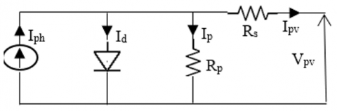
The operation of a photovoltaic cell is inferred from that of a diode PN junction, as well as the equivalent scheme is depicted in Figure 2.
Figure 2. Equivalent electrical scheme of photovoltaic cell
By applying Kirchhoff's current law, the cell's terminal current is [17]:
$\left\{\begin{array}{l}I_{p v}=I_{p h}-I_d-I_p \\ I_d=I_o\left[e^{q\left(\frac{V_{p v}+R_s I_{p v}}{n k T}\right)}-1\right] \\ I_p=\frac{V_{p v}+R_s I_{p v}}{R_p}\end{array}\right.$ (1)
Therefore, the output current Ipv is then written:
$I_{p v}=I_{p h}-I_o\left[e^{q\left(\frac{V_{p v}+R_s I p v}{n k T}\right)}-1\right]-\frac{V_{p v}+R_s I_{p v}}{R_p}$ (2)
where, Iph is the photocurrent (according to the temperature and irradiation), and a term modeling the internal phenomena, Io is the diode reverses saturation current, q is the elementary charge constant, Vpv is the output voltage, Rpand Rs are the cell's parallel and series resistance, respectively, n is the diode ideality factor, between 1 and 5 in practice [18, 19], and k is the Boltzmann constant.
Table 1. Characteristics of PV array
|
Electrical Characteristics |
BP3160S |
|
Optimum operation voltage |
35.1 V |
|
Optimum operation current |
4.55 A |
|
Open-circuit voltage |
44.2 V |
|
Maximum power at STC |
160 W |
|
Short-circuit current |
4.8 A |
|
Peak Efficiency |
16% |
|
Number of Cells |
72 |
|
Maximum System Voltage (V for UL) |
600 V |
|
Maximum System Voltage (V for IEC) |
1000 V |
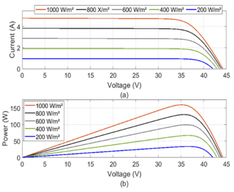
This study is elaborated under MATLAB/Simulink environment. It is composed of 2 PV modules. Every module produces a maximum power of 160 W at 35.1V. Table 1 summarizes its standard electric characteristics. A PV cell is defined by its characteristic curves: current-voltage (I-V) and power-voltage (P-V) [20]. Their characteristic curves are shown in Figures 3-5.
Figure 3 depicted simulation of PV module under constant temperature (T=25°C) and constant irradiation (R=1000W/m²), then Figures 4-5 illustrated simulation PV characteristic with varying irradiation and constant temperature (T=25°C), varying temperature and constant irradiation (T=1000W/m²), respectively.
Figure 3. Close up view curves at R=1000W/m² and T=25℃: Characteristics of (a) I-V and (b) P-V
Figure 4. Characteristics of (a) I-V and (b) P-V
Figure 5. Characteristics of (a) I-V and (b) P-V
2.2 Three-level boost converter
The main components of the PV generator's conversion chain are the DC-DC converters.
They provide interfacing that enables matching between the PV system and the inverter to recover the maximum power of the photovoltaic generator [21-23].
Also, they offer interfaces which enable the PV system and the inverter to operate together to recover the solar generator's maximum power.
Figure 6. Three-level boost converter structure
In this part, an integrated 3-LBC is designed to improve the efficiency of a DC-DC converter used in the photovoltaic application. It is shown in Figure 6.
Although the control of the circuit has been specifically designed for a PV system, in a normal state, it behaves similarly to a conventional topology. The entire array output voltage and one of the motorized currents are used to drive power switch S1 to supply MPPT, as suggested by the misuse of perturb and observe technique. The output voltages of the dc-link electrical devices are balanced by power switch S2. D1 and D2 are forward biased and conducting and each output capacitor is charged during the time when each S1 and S2 is OFF.
The equations below represent the operation mode of the 3-LBC [24]:
$\left\{\begin{array}{l}V_{i n}=V_{p v 1}+V_{p v 2}=\left(L_1+L_2\right) \frac{d i}{d t}+V_{c 1}+V_{c 2} \\ i_{L 1}=C_1 \frac{d V_{c 1}}{d t}+i_{o u t} \\ i_{L 2}=C_2 \frac{d V_{c 2}}{d t}+i_{\text {out }}\end{array}\right.$ (3)
2.3 Mathematical modeling of DSIM
A state-space representation based on the reference frame (α, β) can be used to model the motor. This model is given by [25]:
$\left\{\begin{array}{l}\frac{d}{d t} X_{\alpha \beta}=A X_{\alpha \beta}+B U_{\alpha \beta} \\ Y_{\alpha \beta}=C X_{\alpha \beta}\end{array}\right.$ (4)
where, $X_{\alpha \beta}=\left[\begin{array}{llllll}i_{s \alpha 1} & i_{s \beta 1} & i_{s \alpha 2} & i_{s \beta 2} & \varphi_{r \alpha} & \varphi_{r \beta}\end{array}\right]^T$ represents the state vector, $U_{\alpha \beta}=\left[\begin{array}{llll}u_{s \alpha 1} & u_{s \beta 1} & u_{s \alpha 2} & u_{s \beta 2}\end{array}\right]^T$ denotes the input vector, $Y_{\alpha \beta}=\left[\begin{array}{llll}i_{s \alpha 1} & i_{s \beta 1} & i_{s \alpha 2} & i_{s \beta 2}\end{array}\right]^T$ represents the output vector, $A, B$ and $C$ are matrices that define the electrical drive dynamics.
The electromagnetic torque and the mechanical part can be expressed by the following equation:
$\left\{\begin{array}{l}T_e=\frac{p L_m}{L_m+L_r}\left[\varphi_{r \alpha}\left(i_{s \beta 1}+i_{s \beta 2}\right)-\varphi_{r \beta}\left(i_{s \alpha 1}+\right.\right. \left.\left. i_{s \alpha 2}\right)\right] \\ J_t \frac{d}{d t} \omega+k_f \omega=\left(T_e-T_L\right)\end{array}\right.$ (5)
where, Te,, TL generated and loaded torque, respectively, Lm, Lr mutual and rotor inductances, respectively, φrαβ , isαβ rotor flux and stator current, respectively, Jt denotes the total inertia moment, ω rotor speed, kf friction coefficient.
Taking into account the state-space representation by (4) and using the state vector, we can write the previous system by the following equation:
$\left\{\begin{array}{c}\frac{d}{d t}\left(i_{s \alpha 1}\right)=a_1\left(-R_{s 1} i_{s \alpha 1}-a_2 i_{s \alpha 2}-a_3 \frac{d \varphi_{r \alpha}}{d t}\right)+ \\ b_1 u_{s \alpha 1} \\ \frac{d}{d t}\left(i_{s \beta 1}\right)=a_1\left(-R_{s 1} i_{s \beta 1}-a_2 i_{s \beta 2}-a_3 \frac{d \varphi_{r \beta}}{d t}\right)+ \\ b_1 u_{s \beta 1} \\ \frac{d}{d t}\left(i_{s \alpha 2}\right)=a_4\left(-R_{s 2} i_{s \alpha 2}-a_2 i_{s \alpha 1}-a_3 \frac{d \varphi_{r \alpha}}{d t}\right)+ \\ b_2 u_{s \alpha 2} \\ \frac{d}{d t}\left(i_{s \beta 2}\right)=a_4\left(-R_{s 2} i_{s \beta 2}-a_2 i_{s \beta 1}-a_3 \frac{d \varphi_{r \beta}}{d t}\right)+ \\ b_2 u_{s \beta 2} \\ \frac{d}{d t}\left(\varphi_{r \alpha}\right)=a_5\left(i_{s \alpha 1}+i_{s \alpha 2}\right)-a_6 \varphi_{r \alpha}-a_7 \varphi_{r \beta} \\ \frac{d}{d t}\left(\varphi_{r \beta}\right)=a_5\left(i_{s \beta 1}+i_{s \beta 2}\right)-a_6 \varphi_{r \beta}+a_7 \varphi_{r \alpha}\end{array}\right.$ (6)
where,
$\left\{\begin{array}{l}a_1=\frac{1}{\sigma\left(L_m+L_s\right)}, a_2=\frac{L_m L_r}{L_m+L_r}, a_3=\frac{L_m}{L_m+L_r} \\ a_5=\frac{R_r L_m}{L_m+L_r}, a_6=\frac{a_5}{L_m}, a_7=\omega, a_8=\frac{L_m}{J_m L_r} \\ a_9=-\frac{T_L}{J_m}, a_{10}=\frac{L_m}{L_r}, L_{s 1}=L_{s 2}=L_s \\ \sigma=1-\frac{L_m^2}{\left(L_m+L_s\right)\left(L_m+L_r\right)}, b_1=b_2=a_4=a_1\end{array}\right.$ (7)
2.4 EV dynamic model
The resistant torque is expressed by the EV model, producing an image of resistant forces that oppose the vehicle's motion.
Therefore, the entire force of resistance to the EV's motion can be represented by [26]:
$F_t=F_f+F_a+F_p+F_r$ (8)
with,
$\left\{\begin{array}{l}F_f=1 / 2 \rho C_f A V^2 \\ F_a=1 / 2 \rho C_a A\left(V \pm V_v\right)^2 \\ F_p= \pm m g \sin \left(\alpha_p\right) \\ F_r=C_r m g\end{array}\right.$ (9)
where, Ff: friction resistance, Fa: aerodynamic resistance, Fp: road profile resistance and Fr: rolling resistance, ρ: air density, Cf, Ca, Cr: friction, aerodynamic and rolling resistance coefficient, respectively, A: vehicle cross sectional area, m: vehicle mass, V and Vv: vehicle and wind velocity, respectively.
To emulate the real behavior of the EV, an emulator structure is depicted in Figure 2. It consists of a drive DSIM and a DCM is operating to emulate the dynamic characteristics of EV. The DSIM is supplied by PV system, and using an ANFIS sensor-less control for its speed.
Backstepping control is one of the most reliable nonlinear approaches. It has been used to control lot of types of electric motors [27-29].
Further, the BC technique is a systematic, recursive and a form of non-linear control design [30]. This method may significantly increase the system's stability of the associated Lyapunov function [31]. However, the BC is presented on the basis of the step-by-step construction of the Lyapunov function [32, 33].
The synthesis of this control is achieved in two successive steps:
3.1 Step 1
This first step consists in identifying two errors, which represents the speed and the rotor flux, respectively. In this part, it is assumed that the machine parameters are known and the errors chosen are denoted by: $e_1$ and $e_2$ to define the stabilizing functions.
We define the racking errors by the following equation:
$\left\{\begin{array}{l}e_1=\omega_{r e f}-\omega \\ e_2=\phi_{\text {ref }}-\phi_r\end{array}\right.$ (10)
QBy derivation of (10), we obtain:
$\left\{\begin{array}{l}\dot{e}_1=\dot{\omega}_{\text {ref }}-\dot{\omega} \\ \dot{e}_2=\dot{\phi}_{\text {ref }}-\dot{\phi}_r\end{array}\right.$ (11)
The first Lyapunov candidate function $V_1$ and its derivative $\dot{V}_1$ can be defined by the following equation:
$\left\{\begin{aligned} V_1= & \frac{1}{2}\left(e_1^2+e_2^2\right) \\ \dot{V}_1= & \left(e_1 \dot{e}_1+e_2 \dot{e}_2\right) \\ = & e_1\left[\dot{\omega}_{r e f}-\frac{1}{J_m}\left(a_{10}\left(i_{s \beta 1}+i_{s \beta 2}\right) \dot{\phi}_{r e f}+k_f a_7\right.\right. \\ & \left.\left.+T_L\right)\right]+e_2\left[\dot{\phi}_{r e f}+a_6 \phi_r-a_5\left(i_{s \alpha 1}+i_{s \alpha 2}\right)\right]\end{aligned}\right.$ (12)
According to the Lyapunov stability, when $\dot{V}_1$ is defined negative, the origins $e_1=0$ and $e_2=0$ of the system are asymptotically stable.
Consequently, the following choice will satisfy the tracking objectives:
$\left\{\begin{array}{c}i_{s \beta 1 \text {ref }}+i_{s \beta 2 r e f}=\frac{J_m}{a_{10} \dot{\phi}_{\text {ref }}}\left(k_1 e_1+\dot{\omega}_{\text {ref }}+\frac{k_f}{J_m} a_7\right. \left.+\frac{T_L}{J_m}\right) \\ i_{\text {sa1ref }}+i_{s \alpha 2 r e f}=\frac{1}{a_5}\left(k_2 e_2+\dot{\phi}_{\text {ref }}+a_6 \phi_r\right)\end{array}\right.$ (13)
Therefore, (12) can be rewritten as follows:
$\dot{V}_1=\left(-k_1 e_1^2-k_2 e_2^2\right)<0$ (14)
with, $k_1, k_2$ are positive constants that control the closed loop dynamics which must be chosen to ensure system stability, and these are often acquired by adjustment.
3.2 Step 2
In this stage, the four stator currents generated by the first step are adjusted to establish the control law. In this part, the errors chosen are denoted by: $e_3, e_4, e_5$ and $e_6$. We also provide their error signals by the following equation:
$\left\{\begin{array}{l}e_3=i_{s \beta r e f 1}-i_{s \beta 1} \\ e_4=i_{\text {saref } 1}-i_{s \alpha 1} \\ e_5=i_{s \beta r e f 2}-i_{s \beta 2} \\ e_6=i_{\text {saref } 2}-i_{s \alpha 2}\end{array}\right.$ (15)
Then, the dynamics of errors are expressed as follows:
$\left\{\begin{aligned} \dot{e}_3 & =i_{s \beta r e f 1}-i_{s \beta 1} \\ & =i_{s \beta r e f 1}-b_1 u_{s \beta 1}+\delta_1 \\ \dot{e}_4 & =i_{\text {saref } 1}-i_{s \alpha 1} \\ & =i_{s \alpha r e f 1}-b_1 u_{s \alpha 1}+\delta_2 \\ \dot{e}_5 & =i_{s \beta r e f 2}-i_{s \beta 2} \\ & =i_{s \beta r e f 2}-b_2 u_{s \beta 2}+\delta_3 \\ \dot{e}_6 & =i_{\text {saref } 2}-i_{s \alpha 2} \\ & =i_{\text {saref } 2}-b_2 u_{s \alpha 2}+\delta_4\end{aligned}\right.$ (16)
with,
$\left\{\begin{array}{l}\delta_1=a_1\left[-R_{s 1} i_{s \beta 1}-a_2 i_{s \beta 2}-a_3 \frac{d \varphi_{r \beta}}{d t}\right] \\ \delta_2=a_1\left[-R_{s 1} i_{s \alpha 1}-a_2 i_{s \alpha 2}-a_3 \frac{d \varphi_{r \alpha}}{d t}\right] \\ \delta_3=a_4\left[-R_{s 2} i_{s \beta 2}-a_2 i_{s \beta 1}-a_3 \frac{d \varphi_{r \beta}}{d t}\right] \\ \delta_4=a_4\left[-R_{s 2} i_{s \alpha 2}-a_2 i_{s \alpha 1}-a_3 \frac{d \varphi_{r \alpha}}{d t}\right]\end{array}\right.$ (17)
The Lyapunov function $V_2$ which include these errors $\left(e_3, e_4, e_5\right.$ and $\left.e_6\right)$ and its derivative $\dot{V}_2$ are explained by the following equation:
$\left\{\begin{array}{l}V_2=\frac{1}{2}\left(e_1^2+e_2^2+e_3^2+e_4^2+e_5^2+e_6^2\right) \\ \dot{V}_2=\left(e_1 \dot{e}_1+e_2 \dot{e}_2+e_3 \dot{e}_3+e_4 \dot{e}_4+e_5 \dot{e}_5+e_6 \dot{e}_6\right)\end{array}\right.$ (18)
According to (11) and (16), Eq. (18) can be rewritten as follows:
$\left\{\begin{array}{c}\dot{V}_2=\left[-k_1 e_1{ }^2-k_2 e_2{ }^2-k_3 e_3{ }^2-k_4 e_4{ }^2\right. \left.-k_5 e_5{ }^2-k_6 e_6{ }^2\right]<0 \\ k_3>0, k_4>0, k_5>0, k_6>0\end{array}\right.$ (19)
Therefore, the Lyapunov function derivative will be negative if we impose the control as follows:
$\left\{\begin{array}{l}u_{s \beta r e f 1}=\frac{1}{b_1}\left(i_{s \beta r e f 1}-\delta_1+k_3 e_3\right) \\ u_{\text {s$\alpha$ref } 1}=\frac{1}{b_1}\left(i_{\text {s$\alpha$ref } 1}-\delta_2+k_4 e_4\right) \\ u_{s \beta r e f 2}=\frac{1}{b_2}\left(i_{s \beta r e f 2}-\delta_3+k_5 e_5\right) \\ u_{\text {s$\alpha$ref } 2}=\frac{1}{b_2}\left(i_{\text {s$\alpha$ref } 2}-\delta_4+k_6 e_6\right)\end{array}\right.$ (20)
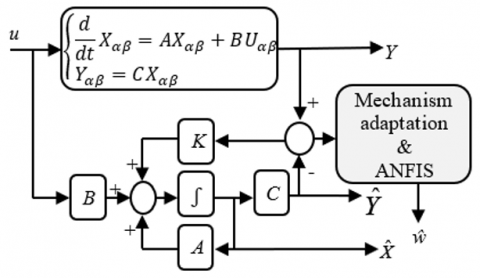
In this case, the state observer is employed to estimate the rotor speed and flux components of DSIM by including an adaptive mechanism based on the ANFIS. The proposed scheme of the LO is shown in Figure 7.
The observer equation is given by:
$\left\{\begin{array}{l}\frac{d}{d t}\left(\hat{X}_{\alpha \beta 1,2}\right)=A \hat{X}_{\alpha \beta 1,2}+B U_{\alpha \beta 1,2}+K_L\left(Y_{\alpha \beta 1,2}\right. \left.-\hat{Y}_{\alpha \beta 1,2}\right) \\ Y_{\alpha \beta 1,2}=C X_{\alpha \beta 1,2}\end{array}\right.$ (21)
where, KL is the observer gain matrix.
By using PI controller for speed adaptive mechanism, we obtain:
$\widehat{\omega}=k_p\left(\lambda_1 \hat{\varphi}_{r \beta}-\lambda_2 \hat{\varphi}_{r \alpha}\right)+k_i \int\left(\lambda_1 \hat{\varphi}_{r \beta}-\lambda_2 \hat{\varphi}_{r \alpha}\right) d t$ (22)
where, λ1 and λ2 are errors between the estimated and real components. kp and ki are proportional and integral positive gains.
Figure 7. ANFIS-LO scheme
4.1 ANFIS-PI controller
ANFIS is employed to emulate, both the neural and fuzzy inference system behavior. Also, it looks like adaptive network emulator of the adaptive Takagi-Sugeno’s fuzzy controllers, witch defined for fuzzy inference systems (FIS). The ANFIS can utilize the Takagi-Sugeno (TS) fuzzy model due to its efficiency. The controller seeks for smoothless as a result of Artificial Neural Network (ANN) backpropagation algorithms.
The proposed ANFIS uses two inputs: the first for the error and the second for the change of error. The general scheme of an ANFIS of this system is shown in Figure 8. For the first layer, MFs will be described in each of the inputs. In the second layer, each node calculates the firing strength of the rule which is normalized in the third layer. TS fuzzy model contains two common rules, which are depicted as:
I: if e=A1 and Δe=B1, then f1 = a1 e=+b1Δe + c1
II: if e=A2 and Δe=B2, then f2 = a2 e=+b2Δe + c2
where, Ai, Bi and ai, bi, ci are fuzzy sets input and defined in the training plant, respectively.
Figure 8. ANFIS scheme with two parameter inputs
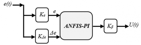
In this section, the main contribution is to clarify an ANFIS-PI controller which can follow the reference speed.
However, this structure can also provide high performance of the developed sensor-less control with mechanism adaptation of the LO. As well as providing better sensitivity, and ameliorate the closed-loop system’s overall stability. The control structure for DSIM speed regulation with an ANFIS is presented in Figure 9.
Figure 9. Structure of ANFIS based PI controller
The control output can be deduced as follows:
$u(t)=\left[k_e e(t)+k_{\Delta e} e(t)\right] k_\beta$ (23)
The parameters of Eq. (22) are determined using the following expression:
$\left\{\begin{array}{l}k_p=k_e k_\beta \\ k_i=k_\beta\end{array}\right.$ (24)
where, Ke, KΔe, and Kβ are the inputs and output scaling factors, respectively. The training, checking and testing data for the ANFIS controller are obtained from the fuzzy based-PI controller. The fuzzy controller uses a TS type FIS with two inputs and a single output. Figure 10 shows the training data for the ANFIS controller.
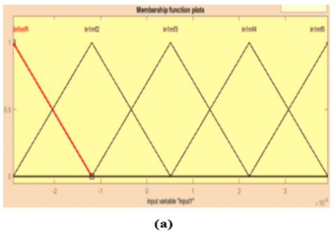
The inputs membership functions obtained after training are shown in Figures 11(a) and (b). The epoch’s number is 100 for training. The MF’s number for the input variables is 5 and 3, and the number of rules is 15. Therefore, the ANFIS used here contains a total of 61 fitting parameters, of which 16 (2*5+2*3) are the premise parameters and 45 (3*15) are the consequent parameters. Then, the Figure 12 shows the ANFIS model structure.
Figure 10. The training error
Figure 11. Membership functions of input variables: (a) e and (b) Δe
Figure 12. ANFIS controller structure
The main objective of this section is to investigate the performance of the suggested ANFIS sensor-less controller with backstepping technique for the DSIM drive, which the nominal parameters are illustrated in Table A1 (see Appendix).
5.1 Comparisons between the ANFIS-LO controller and conventional LO controller
In this study, to validate the proposed approach and demonstrate its effectiveness, we subjected our DSIM to a load varying over time. We also introduced parametric variations, order of +50% at t = 6s. The simulation results are given in Figures 13-24. On the other hand, this simulation study will be based on two scenarios: firstly, it is intended that the temperature remains constant and the irradiation has the profile illustrated in the Figure 13. Secondly, the temperature has the profile presented in the Figure 19 and the irradiation is supposed to be constant. For both scenarios, we will discuss the transient behavior as well as the steady-state response.
Figure 13. Irradiation profile
5.1.1 The first scenario
In this case, the temperature T=25℃ and an irradiation varying between 200W/m² to 1000W/m², the obtained results of this scenario are shown in Figures 13-18.
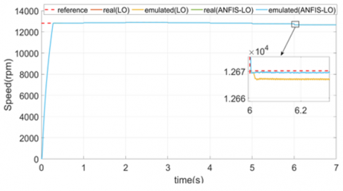
The analysis reveals the electromagnetic torque and rotor flux follow well their references. Decreased irradiation level causes the DSIM's speed decrease, and increased irradiation level causes the speed to increase. From the simulation results shown in Figure 15, it is easy to see that the speed response in the first scenario is very good, so the speed error is nearly zero in the stable mode. ANFIS sensor-less controller can provide a very good dynamic response when the EV is operating, as shown in Figure 18.
Figure 14. Output voltage of boost converter
Figure 15. Reference, real and emulated rotation speed (upper plot) in case of rotor resistance variation at t = 6s, and speed error (lower plot)
Figure 16. DSIM reference and real rotor flux
Figure 17. DSIM real and emulated load torque
Figure 18. Electric vehicle linear speed
5.1.2 The second scenario
In this case, the irradiation R=1000W/m² and the temperature varying between T=15℃ to T=55℃, the obtained results of this scenario are shown in Figures 19-24.
Figure 19. Temperature profile
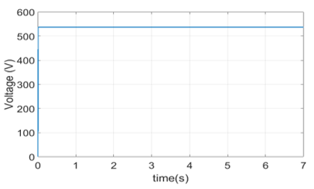
It can be seen, from the Figure 20, that the boost converter produces a fixed voltage to power the inverter.
Figure 20. Output voltage of boost converter
According to the simulation results above, we can see the good ANFIS sensor-less control performance for estimated speed tracking in different weather conditions. The rotor flux is nearly identical to the reference. So, the obtained results are sufficient and confirmed the efficiency of the suggested control.
Acually, the proposed ANFIS-LO controller improves the performance metrics in both transient and steady state response in comparison to the conventional LO as shown in Table 2.
Table 2. Comparison of ANFI-LO and LO control strategies
|
Control Strategies |
Estimation Accuracy |
Convergence Speed |
Robustness to Parameter Variations |
|
LO |
+ |
+ |
- |
|
ANFIS-LO |
++ |
++ |
++ |
Figure 21. Reference, real and emulated rotation speed (upper plot) in case of rotor resistance variation at t = 6s, and speed error (lower plot)
Figure 22. DSIM reference and real rotor flux
Figure 23. DSIM real and emulated load torque
Figure 24. Electric vehicle linear speed
This paper has proposed a sensor-less BC using the LO with an ANFIS adaptation mechanism of DSIM drive aimed at applying electric vehicles fed by PV. To test the system’s performance, we have used two scenarios, decreased and increased by variation in irradiation and temperature level, in the simulation results. Thus, these results have demonstrated the efficiency and the performance of the suggested scheme for the transient behavior as well as the steady-state response even at different reference speed with EV. In Addition, we have highlighted the performance of the suggested control.
The projected work will address the development of the proposed control by using other techniques.
|
ANFIS |
Adaptive neuro-fuzzy inference system |
|
DSIM |
Double stator induction motor |
|
EV |
Electric vehicle |
|
PV |
Photovoltaic |
|
MPPT |
Maximum power point tracker |
|
P&O |
Perturb and Observe |
|
LO |
Luenberger Observer |
|
Greek symbols |
|
|
$\alpha$ |
Reference frame of $\alpha$ axe |
|
$\beta$ |
Reference frame of $\beta$ axe |
|
$\sigma$ |
Dispersion coefficient |
|
$\rho$ |
Air density, Kg/m3 |
|
Subscripts |
|
|
S |
Series |
|
sh |
Shunt |
|
ph |
Photon |
|
s |
Stator |
|
r |
Rotor |
|
L |
Load |
Table A1. DSIM parameters
|
Nominal Parameter |
Used Value |
|
DSIM nominal power |
4.5Kw |
|
Rotor/Stator resistance |
3.72Ω |
|
Rotor inductance |
0.006H |
|
Stator inductance |
0.022H |
|
Magnetizing inductance |
0.3672H |
|
Inertia moment |
0.0625kg.m2 |
|
Friction coefficient |
0.001N.m.s/rad |
[1] Azib, A., Ziane, D., Rekioua, T., Tounzi, A. (2016). Robustness of the direct torque control of double star induction motor in fault condition. Revue Roumaine Des Sciences Techniques—Série Électrotechnique ET Énergétique, 61(2): 147-152. http://www.revue.elth.pub.ro/index.php?action=mai&year=2016&issue=2.
[2] Himour, K., Yahiaoui, A., Iffouzar, K. (2020). Comparison of different control strategies of multilevel inverters used to fed a dual star induction machine. Journal Européen des Systèmes Automatisés, 53(4): 525-532. https://doi.org/10.18280/jesa.530411
[3] Beghdadi, A., Bentaallah, A., Abden, A. (2021). Optimization of sliding mode with MRAS based estimation for speed sensorless control of DSIM via GWO. Przegląd Elektrotechniczny, 6: 21-29. http://doi.org/10.15199/48.2021.06.04
[4] Chen, Q., Liao, C., Ouyang, A., Li, X., Xiao, Q. (2016). Research and development of in-wheel motor driving technology for electric vehicles. International Journal of Electric and Hybrid Vehicles, 8(3): 242-254. http://doi.org/10.29354/diag/125307.
[5] Terfia, E., Rezgui, S.E., Mendaci, S., Gasmi, H., Benalla, H. (2023). Optimal fractional order proportional integral controller for dual star induction motor based on particle swarm optimization algorithm. Journal Européen des Systèmes Automatisés, 56(2): 345-353. https://doi.org/10.18280/jesa.560220
[6] D Derbane, A., Tabbache, B., Ahriche, A. (2021). A fuzzy logic approach based direct torque control and five-leg voltage source inverter for electric vehicle powertrains. Revue Roumaine Des Sciences Techniques—Série Électrotechnique ET Énergétique, 66(1): 15-20. http://www.revue.elth.pub.ro/index.php?action=main&year=2021&issue=1.
[7] Frikha, M.A., Croonen, J., Deepak, K., Benômar, Y., El Baghdadi, M., Hegazy, O. (2023). Multiphase motors and drive systems for electric vehicle powertrains: State of the art analysis and future trends. Energies, 16(2): 768. https://doi.org/10.3390/en16020768.
[8] Bang, J.S., Shim, H., Park, S.K., Seo, J.H. (2009). Robust tracking and vibration suppression for a two-inertia system by combining backstepping approach with disturbance observer. IEEE Transactions on Industrial Electronics, 57(9): 3197-3206. https://doi.org/10.1109/TIE.2009.2038398
[9] Hamonangan, J.A. (2019). Review perbandingan teknik Maximum Power Point Tracker (MPPT) untuk sistem pengisian daya menggunakan sel surya. Jurnal Teknologi Dirgantara, 16(2): 111-122. http://doi.org/10.30536/j.jtd.2018.v16.a2998
[10] Khemili, F.Z., Lefouili, M., Bouhali, O., Rizoug, N., Bekrar, L. (2022). Dual three phase multilevel space vector modulation control of diode clamped inverter for dual star induction motor drive. Journal Européen des Systèmes Automatisés, 55(5): 603-613. https://doi.org/10.18280/jesa.550505
[11] Beltran, B., Benbouzid, M., Ahmed-Ali, T. (2012). Second-order sliding mode control of a doubly fed induction generator driven wind turbine. IEEE Transactions on Energy Conversion, 27(2): 261-269. https://doi.org/10.1109/TEC.2011.2181515.
[12] Yamaguchi, M., Masuda, T., Nakado, T., Yamada, K., Okumura, K., Satou, A., Ota, Y., Araki, K., Nishioka, K., Kojima, N., Ohshita, Y. (2023). Analysis for expansion of driving distance and CO2 emission reduction of photovoltaic-powered vehicles. IEEE Journal of Photovoltaics, 13(3): 343-348. https://doi.org/10.1109/JPHOTOV.2023.3242125
[13] Yamaguchi, M., Nakamura, K., Ozaki, R., Kojima, N., Ohshita, Y., Masuda, T., Okumura, K., Satou, A., Nakado, T., Yamada, K., Tanimoto, T., Zushi, Y., Takamoto, T., Araki, K., Ota, Y., Nishioka, K. (2022). Analysis for the potential of high-efficiency and low-cost vehicle-integrated photovoltaics. Solar RRL, 7(8): 2200556. http://doi.org/10.1002/solr.202200556.
[14] Kronthaler, L., Maturi, L., Moser, D., Alberti, L. (2014). Vehicle-integrated photovoltaic (VIPV) systems: Energy production, diesel equivalent, payback time; an assessment screening for trucks and busses. In 9th International Conference on Ecological Vehicles and Renewable Energies (EVER), Monte-Carlo, Monaco, pp. 1-8. https://doi.org/10.1109/EVER.2014.6844150
[15] Karami, N., Moubayed, N., Outbib, R. (2017). General review and classification of different MPPT Techniques. Renewable and Sustainable Energy Reviews, 68(1): 1-18. https://doi.org/10.1016/j.rser.2016.09.132
[16] Antonello, R., Carraro, M., Costabeber, A., Tinazzi, F., Zigliotto, M. (2017). Energy-efficient autonomous solar water pumping system for permanent-magnet synchronous motors, IEEE Transactions on Industrial Electronics, 64(1): 43-51. https://doi.org/10.1109/TIE.2016.2595480
[17] Mei, Q., Shan, M., Liu, L., Guerrero, J.M. (2010). A novel improved variable step-size incremental-resistance MPPT method for PV systems. IEEE Transactions on Industrial Electronics, 58(6): 2427-2434. http://doi.org/10.1109/TIE.2010.2064275
[18] Ishaque, K., Salam, Z., Taheri, H., Shamsudin, A. (2011). Maximum power point tracking for PV system under partial shading condition via particle swarm optimization. In 2011 IEEE Applied Power Electronics Colloquium (IAPEC), Johor Bahru, Malaysia, pp. 5-9. http://doi.org/10.1109/IAPEC.2011.5779866
[19] Shaiek, Y., Smida, M.B., Sakly, A., Mimouni, M.F. (2013). Comparison between conventional methods and GA approach for MPPT of solar PV generators. Solar Energy, 90: 107-122. http://doi.org/10.1016/j.solener.2013.01.005
[20] Aouna, N., Bailek, N. (2019). Evaluation of mathematical methods to characterize the electrical parameters of photovoltaic modules. Energy Conversion and Management, 193: 25-38. https://doi.org/10.1016/j.enconman.2019.04.057
[21] Benamrane, K., Abdelkrim T., Benlahbib, B., Bouarroudj, N., Lakhdari, A., Borni, A., Bahri, A. (2022). New configuration of five-level NPC inverter with Three-Level Boost converter for photovoltaic solar energy conversion. Journal Européen des Systèmes Automatisés, 55(4): 519-525. https://doi.org/10.18280/jesa.550411
[22] Motahhir, S., El Hammoumi, A., El Ghzizal, A. (2020). The most used MPPT algorithms: Review and the suitable low-cost embedded board for each algorithm. Journal of Cleaner Production, 246: 118983. http://doi.org/10.1016/j.jclepro.2019.118983
[23] Li, X., Wen, H., Hu, Y., Du, Y., Yang, Y. (2021). A comparative study on photovoltaic MPPT algorithms under EN50530 dynamic test procedure. IEEE Transactions on Power Electronics, 36(4): 4153-4168. https://doi.org/10.1109/TPEL.2020.3024211
[24] Ribeiro, E., Cardoso, A.J.M., Boccaletti, C. (2013). Fault-Tolerant strategy for a photovoltaic DC–DC converter. IEEE Transactions on Power Electronics, 28(6): 3008-3018. http://doi.org/10.1109/TPEL.2012.2226059
[25] Ayala, M., Gonzalez, O., Rodas, J., Gregor, R., Rivera, M. (2016). Predictive control at fixed switching frequency for a dual three-phase induction machine with Kalman filter-based rotor estimator. In IEEE International Conference on Automatica (ICA-ACCA), Curico, Chile, pp. 1-6. http://doi.org/10.1109/ICA-ACCA.2016.7778449
[26] Roubache, T., Chaouch, S., Said, M.S.N. (2016). Sensorless fault-tolerant control of an induction motor based electric vehicle. Journal of Electrical Engineering and Technology, 11(5): 1423-1432. http://doi.org/10.5370/JEET.2016.11.5.1423
[27] Khadar, S., Kouzou, A., Rezzaoui, M., Hafaifa, A. (2016). Five phase induction motor under partial stator winding short-circuit. Periodica Polytechnica Electrical Engineering and Computer Science, 64(1): 2-19. https://doi.org/10.3311/PPee.14306
[28] Trabelsi, R., Khedher, A., Mimouni, M.F., M'sahli, F. (2012). Backstepping control for an induction motor using an adaptive sliding rotor-flux observer. Electric Power Systems Research, 93: 1-15. https://doi.org/10.1016/j.epsr.2012.06.004
[29] Berrezzek, F., Benheniche, A. (2021). Backstepping based nonlinear sensorless control of induction motor system. Journal Européen des Systèmes Automatisés, 54(3): 495-502. https://doi.org/10.18280/jesa.540313
[30] Boughazi, O., Boumedienne, A., Glaoui, H. (2014). Sliding mode backstepping control for induction motor. International Journal of Power Electronics and Drive Systems, 4(4): 481-488. http://doi.org/10.11591/ijpeds.v4i4.6532
[31] Hosseyni, A., Trabelsi, R., Iqba, A., Mimouni, M.F. (2015). Backstepping control for a five-phase permanent magnet synchronous motor drive. International Journal of Power Electronics and Drive System, 6(4): 842-852. http://doi.org/10.11591/ijpeds.v6.i4.pp842-852
[32] Vaidyanathan, S., Azar, A.T. (2021). An introduction to backstepping control. In Backstepping Control of Nonlinear Dynamical Systems, Academic Press, pp. 1-32. https://doi.org/10.1016/B978-0-12-817582-8.00008-8
[33] Taoussi, M., Karim, M., Bossoufi, B., Hammoumi, D., Lagrioui, A. (2015). Speed backstepping control of the doubly-fed induction machine drive. Journal of Theoretical and Applied Information Technology, 74(2): 189-199. http://www.jatit.org/volumes/seventyfour2.php.