Abdulkader M. Saeed*![]() | Khalida S. Rijab
| Khalida S. Rijab
© 2023 IIETA. This article is published by IIETA and is licensed under the CC BY 4.0 license (http://creativecommons.org/licenses/by/4.0/).
OPEN ACCESS
The integration of a PID controller into the A* algorithm presents a novel approach to enhance water boat path planning efficiency. This fusion leverages the precision of the PID controller to fine-tune the navigation decisions made by the A* algorithm, optimizing trajectory adjustments and overcoming challenges posed by dynamic water environments. The PID controller dynamically adjusts the boat's heading based on real-time feedback, ensuring smoother path execution and faster convergence towards the optimal route. This innovative synergy between a classical pathfinding algorithm and a feedback control system addresses the complexities of water-based scenarios, where unpredictable currents, obstacles, and varying conditions necessitate adaptive strategies. The proposed PID-enhanced A* algorithm not only enhances path planning accuracy but also exhibits improved resilience in the face of environmental uncertainties, making it a promising solution for efficient and reliable autonomous watercraft navigation in diverse and challenging aquatic settings. the results show that the A* algorithm with PID controller is superior to the original A* without PID controller with respect to mean path length and standard deviation with a reduction of up to 23% which leads to improved path planning for proposed environment.
UWB, path planning, avoid obstacles, A* algorithm, PID controller
Navigating water bodies poses unique challenges for autonomous boats, demanding sophisticated algorithms that can adapt to dynamic and unpredictable environments. This introduction delves into the integration of a PID (Proportional-Integral-Derivative) controller with the A* algorithm, a renowned pathfinding technique, to enhance the efficiency of water boat path planning. This fusion of classical and control methodologies aims to overcome the intricacies associated with water-based scenarios, including fluctuating currents, obstacles, and varying conditions [1].
The A* algorithm, widely acclaimed for its effectiveness in pathfinding, serves as the foundational framework for this innovative approach. Known for its ability to find the shortest path between two points on a grid, A* employs a heuristic function to guide the search, efficiently exploring potential routes. However, water environments introduce a layer of complexity, where the dynamic nature of currents and the presence of obstacles demand real-time adaptability [2].
Enter the PID controller—an integral component of many control systems, renowned for its capacity to fine-tune performance based on continuous feedback. By integrating a PID controller into the A* algorithm, we aim to imbue the path planning process with a dynamic responsiveness that mirrors the challenges inherent in aquatic settings.
UWB was very necessary, especially in war operations, delivery the goods, merchandise and rescue operations for illegal immigrants, especially those stranded in the seas and oceans. A variety of boat models utilized for numerous applications are depicted in Figure 1.
The essence of the PID controller lies in its ability to continuously adjust a system's behavior to maintain or reach a desired state. In the context of water boat path planning, this translates to real-time modifications of the boat's heading. The Proportional component responds to the current error, the Integral component addresses accumulated past errors, and the Derivative component anticipates future trends. This triad of control elements works in harmony to optimize trajectory adjustments, ensuring that the boat navigates through water with precision and adaptability [3]. The synergy between the A* algorithm and the PID controller becomes particularly potent when addressing the unpredictable nature of water environments. The A* algorithm excels at exploring possible paths, but the PID controller introduces a layer of intelligence by refining the decisions made during this exploration. It acts as the conductor orchestrating the boat's movements, considering real-time feedback to make informed adjustments in response to changing conditions. Efficiency in water boat path planning hinges on the system's ability to adapt swiftly to unforeseen challenges. The dynamic integration of the PID controller introduces a level of responsiveness that goes beyond the static nature of traditional pathfinding algorithms. This dynamic adjustment not only enhances the precision of navigation but also accelerates the convergence towards the optimal route [4].
The challenges posed by water environments extend beyond the navigational aspects, encompassing factors such as fluctuating currents and unexpected obstacles. The PID-enhanced A* algorithm addresses these challenges by enabling the boat to dynamically respond to environmental cues. It transforms the boat's path planning from a predetermined course to an adaptive journey, were real-time feedback guides decisions, making it resilient to the uncertainties of aquatic settings. In summary, the integration of a PID controller with the A* algorithm for water boat path planning represents a significant leap forward in autonomous aquatic navigation. By combining the exploratory prowess of the A* algorithm with the dynamic adaptability of the PID controller, this approach promises efficient, precise, and resilient path planning in the face of the unpredictable nature of water environments. This innovative fusion holds the potential to revolutionize autonomous watercraft navigation, opening new frontiers in applications ranging from environmental monitoring to search and rescue operations.
The remainder of this paper is organized as follows: previous path planning work is presented in section 2. Section 3 described the idea of planning, obstacle avoidance and A* algorithm. section 4 describes the proposed algorithm; section 5 described the hardware item; section 6 described evaluation of numerical parameters required. section 7 described the proposed environment. section 8 described the results obtained for standard A* and improved A* with PID controller. Finally, the conclusion is presented in section 9.
Figure 1. Serval types of UWB
Many techniques were proposed in order to develop an optimal USV path for various missions. For path planning with obstacles in an enclosed environment, the robotics group at MIT uses the belief roadmap method (BRM), which contains a prediction model [5].
In order to avoid collisions, Huang et al. [6] developed a revolutionary ant colony optimization (ACO) method that takes both static and moving obstacles into account.
Ozkan et al. [7] focused on using unmanned aerial vehicles (UAVs) to generate a ground map of a flooded urban environment for rescue operations. The ground map is generated by processing an aerial image taken from the UAV. The generated ground map is then used to plan the path of a rescue boat to reach the target location. The study analyses three different path planning algorithms to find the most suitable one for flooded urban. The study used an aerial image taken from Houston during Hurricane Harvey in 2017 to generate a ground map. The proposed image processing techniques were used to segment the image and model the ground map. The study then analyzed three different path planning algorithms: A*, GA, and PRM. Simulations were performed to evaluate the performance of these algorithms. The results showed that the PRM algorithm was the most suitable for flooded urban environments.
Li and Zhang [8] proposed improve traditional ant colony algorithm for unmanned boat include optimizing the state transiting rules and dynamically adjusting the pheromone volatilization coefficient using a Gaussian function. To verify the effectiveness of the optimization algorithm, it used MTLAB2018a to simulate and compare between two algorithms. The comparison showed that the shortest path of the basic ant colony algorithm was 15445.1154, and the shortest path of the optimized ant colony algorithm was 15264.0604. This indicates that the optimized path of the improved ant colony algorithm is better than that of the basic ant colony algorithm.
The research [9] proposed an improved collision avoidance algorithm for unmanned surface vehicles (USVs) that combines an improved artificial potential field and ant colony optimization. The algorithm uses a power function based on the change of the distance to the obstacle to solve the problem of frequent steering and overshoot of USV's control system during collision avoidance. Results show the proposed method is more efficient and capable of avoiding obstacles through route planning, particularly in the presence of large disturbances. The research also presents an evaluation method for USV's collision avoidance based on the minimum safety distance and stability parameters. The results of simulation and experiment demonstrate the effectiveness and robustness of the propose.
Xiao et al. [10] proposed using a combination of an Unmanned Surface Vehicle (USV) and an Unmanned Aerial Vehicle (UAV) to automate marine mass casualty incident search and rescue. The system uses the UAV to provide responders with an overhead view of the field and automate the rescue process. The paper mentions the use of PID control when the error angle is within the 30° threshold to achieve a desired heading for the USV. The throttle is set to 60% of the maximum value. The PID control is used to ensure that the USV moves in the correct direction and maintains a stable heading.
Zhang and Li [11] applied optimization techniques to remove unnecessary nodes, minimize the length of the path, and lessen the number of inversion sites in both directions. Finally, a cubic spline function is added to smooth the route simulation. The results show that the smoothness, inflection points, and path length of the A* algorithm are effectively optimized. But compared to other algorithms, the journey is still rather long.
In this part, path planning and obstacles avoidance system described such as:
3.1 Path planning and obstacles avoidance
The environment includes number of obstacles such as, O1, O2, ..., On. It is spreading in the environment and their have a site coordinate are presented as (X1, Y1), (X2, Y2). Obstacles can be classified into static and dynamic. When it is fixed, that means speed may be zero, and if it is moving, it has speed along the x and y axes. Each obstacle has differenced speed from another obstacle and is different to the speed of the boat. Speed and location of the obstacle are unknown for the boat. The boat needs to understand all obstacles information such as type, size, speed and any direction it found. If the boat does not know where the obstacle and how its speed and position, it must be needed some device to help boat to collect environmental data. The boat is supported with an ultrasonic sensor in order to detect an obstacle in an environment. Also, it equipped 180-degree proximity information. When the boat moves to a new position, first it reads the data obtaining from sensor in order to calculate the distance between obstacles and boat. it must be needed some device to help boat to collect environmental data. The boat is supported with an ultrasonic sensor that equipped 180-degree proximity information. When the boat moves to a new position, first it reads the data obtaining from sensor in order to calculate the distance between obstacles and boat.
The boat, which obtaining information about obstacle within region, to determine the distance between an obstacle and a boat, and to estimate the direction of the moving obstacle [12]. If the position of the obstacle fixed, means that it is static. Or, it is dynamic. Direction of the obstacle is estimated by helping sensor and the boat will choose the next way depending on environment information. When the obstacle moves toward boat path, a boat will move to avoid hit with obstacle. moreover, if the distance between boat and an obstacle increased continuously that means the dynamic moves far from the boat. Otherwise, obstacle may be moved towards the boat. The path planning model for the proposed system is shown in Figure 2.
Figure 2. Path planning and obstacle avoidance model
Where, dR0: distance from boat to obstacle and dRG: Distance from boat to goal.
Parameter dR0 and dRG are used to describe the distance between a boat and an obstacle, and the distance between the boat and the goal position, respectively, using the distance formula, which is expressed as shows:
$\mathrm{dR}_0=\sqrt{(X s-X o b s)^2+(Y s-Y o b s)^2}$ (1)
$\mathrm{dR}_{\mathrm{G}}=\sqrt{(X s-X g)^2+(Y s-Y g)^2}$ (2)
where, Xg and Yg are the goals coordinates in the environment, Xs and Ys, described the current boat coordinate, and Xobs and Yobs, described the obstacles coordinates in the environment.
The route planning method involves determining the best route to take from one place to another. Route planning problems are widely observed in transportation logistics, automobile navigation systems, computer communication networks, and decision-making systems for people fleeing disasters [13]. Applications of network design and graph theory depend on finding optimal or near-optimal paths [14]. The two main parts of optimal routing algorithms are heuristic and optimization [15]. The ideal approach is ineffective for real-time positioning systems [16] because it increases the time complexity when using complex PRM, despite the fact that heuristic and metaheuristic algorithms more efficient in navigating the search space and finding the optimal path like a monster algorithm. The many heuristic algorithms accessible in the study [17] include techniques for local multiresolution search and the best-first search algorithm, to name just a few. On the other hand, one of the most crucial applications that prevent collisions and keep the vehicle moving in the direction of the aim is obstacle avoidance. Obstacle avoidance is frequently performed in a social setting. Path planning, on the other hand, entails determining an obstacle-free path before guiding the boat along it.
3.2 A* algorithm
A heuristic approach algorithm is the A* algorithm. Peter Hart, Nils Nilsson, and Bertram Raphael, researchers of the Stanford Research Institute, first presented it in 1968 [18]. While the A* algorithm determines the shortest path, the total cost is calculated using the formula below.
$\mathrm{F}(\mathrm{x})=\mathrm{G}(\mathrm{x})+\mathrm{H}(\mathrm{x})$ (3)
The distance function G(x) represents the cost of the distance traveled from a starting point to a desired location on a map. It can be calculated using the identified path. The estimated cost of going from any square to the target square is given by the expression H(x). This is merely an educated guess and is referred to as a heuristic. Because many barriers (walls, water, etc.) may arise on the path, the true distance cannot be determined until the route is located. Where F(x) represents the entire cost.
The heuristic function is the most important contributor to the A* algorithm's success. There are several methods for calculating heuristic distance.
Some of these are the Euclidean distance and the Manhattan distance. Table 1 shows formulas for computing the Manhattan and Euclidean distances.
Table 1. Distance function based on Heuristic
|
Heuristic Function |
Equation |
|
Euclidean |
h(x)=[(Bx-Ax)2 + (By-Ay)2]1/2 |
|
Manhattan |
h(x)=|Bx - Ax| +|By - Ay| |
The A* algorithm is well-suited for water boat path planning due to its efficient and effective nature in finding optimal paths in a grid-based environment. Here are several reasons why the A* algorithm is a suitable choice such as: optimality, heuristic guidance and adaptability to dynamic environment.
3.3 Basic work for A* algorithm
A common pathfinding technique used in artificial intelligence and robotics to locate the shortest route between two locations in a graph or grid is called the A* algorithm. Although it is based on the Dijkstra's algorithm, it also has a heuristic function to direct the search in the direction of the objective. The A* algorithm's fundamental phases are listed below:
Step1: Set up the closed list and the open list from scratch. The initial node is present in the open list, whereas the closed list is empty.
Step2: Set the beginning node's G- and F-score to 0. The anticipated total cost of the path through the current node to the destination node is represented by the F-score, while the G-score represents the cost to get to the current node from the starting node.
Step3: While the open list is not empty, do the following:
Step4: Stop the search and return failure if the goal node cannot be reached from the beginning node.
The Manhattan distance or the Euclidean distance between the current node and the desired node is often the heuristic function utilized in the A* method. It directs the search in the direction of the goal by giving priority to nodes that are closer to the goal and is used to estimate the remaining cost of the path from the current node to the goal node. When calculating the heuristic distance, it's important to keep in mind that the A* method will be more accurate and quicker more closely the heuristic distance is actual. The A* algorithm's flowchart is shown in Figure 3.
In general, the A* algorithm examines the nodes nearby before starting its computation from the predetermined beginning nodes. Open and closed lists are created after the review. The nodes to be explored are selected from the open list, which contains the nodes that are close to the nodes being researched. The list containing the investigated nodes is known as the closed list.
Figure 3. Flowchart of the A* algorithm
The nodes under inquiry are not assessed again to prevent the algorithm from looping. The open list's lowest cost points are explored after researching the starting point, and the process is then continued until the end point is reached. The heuristic function makes sure that the algorithm moves accurately and diverges-free towards the objective point. When the end point is added to the closed list, the objective has been found and the process is finished. The route is formed by returning to the starting point by following the parent points from the target point.
The PID (Proportional-Integral-Derivative) controller is a feedback system used in control engineering. It comprises three components: Proportional (P), Integral (I), and Derivative (D), working together to regulate a system by adjusting its output based on the error signal.
As shown in previous studies, the aim of PID controller made a system to be stable. Because of the waves water generated from boat when it moves will make a boat to avoid the original path. In order to solve this problem a PID controller used to make a boat to be stable on the path in order to arrive from start point to a target point with less time, Figure 4 show a part of the basic work PID controller for an automated boat.
The time constant formula of the PID controller is given as in Eq. (4) [19].
$G_{\mathrm{c}}=K_{\mathrm{p}}\left(1+\frac{1}{T_i s}+T_d s\right)$ (4)
where, Kp proportional gain which used to increase the system response speed and reduce steady-state error [20], and Ki integral gain which used to eliminate the steady-stat error at all [Ki = Kp / (Ti integral time constant)] but it produces unwanted increase on the response overshoot, while Kd derivative gain used to reduce the system response overshoot [Kd = Kp * (Td derivative time constant)] [21].
Figure 4. PID controller system
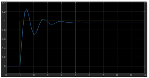
By using MATLAB R2022a the parameters calibration for PID controller in many cases in order to choose the optimal case and are set (Kp = 4.5, Ki = 2.3 and Kd = 1) as shown in Figure 5.
(a)
(b)
(c)
Figure 5. The calibration and effect for response: (a) Kp = 3, Ki = 2 and Kd = 3, (b) Kp = 4, Ki = 1 and Kd =5 and (c) Kp = 4.5, Ki = 2.3 and Kd = 1
Figure 6. Flowchart part for PID controller with proposed algorithm
After that, an automated boat moved from start point to end point with smooth path so without obstacle collision. Figure 6 show the flowchart of a part automated boat using PID controller.
In this section we will be described in details the main compound required to implement an automated boat such as:
5.1 3D printer
Progressive material addition is used in digital fabrication technology, also referred to as 3D printing or additive manufacturing, to create actual objects from a geometric representation. A fast-evolving technology is 3D printing. Today, 3D printing is widely used all around the world. The use of 3D printing technology for mass production and customization of any kind is growing quickly. In the fields of agriculture, health care, the automobile industry, locomotive manufacturing, and aviation, there are various types of open-source designs. By depositing material layer by layer, 3D printing technology may produce an object straight from a computer-aided design [22].
The boat was printed using a 3D printer using a solid works program that shows the Figure 7 3D printer and it makes the boat.
Figure 7. Printing a boat using 3d printer
The boat was printed with pure engineering specifications and measurements shown, as shown in Figure 8.
(a)
(b)
Figure 8. (a) The measurement for the boat, and (b) show the boat after printing using 3d printer
5.2 Raspberry pi 4
Raspberry pi 4 is an integrated computer made of one electronic chip that contains the components of a traditional computer, which is a single-core CPU data processor at 700 MHZ, and a dual-core GPU graphics processor at 250 MHZ capable of operating HD movies and 3D games with a random memory of up to RAM 512 Mb. In addition, the raspberry pi consists of 40 digital pins that are used to control electronic and electrical parts. And various sensors. All these capabilities are on a small chip only, which is what is known as "SOC: System on Chip". This computer is operated with open-source Linux systems, Figure 9 shows the raspberry pi 4 used to proposed system. The Raspberry pi 4 specifications is shown in Table 2.
Figure 9. Raspberry pi 4 model A
Table 2. Specifications of a raspberry pi 4 board
|
Parameters |
Description |
|
Microcomputer |
Raspberry pi 4 |
|
Power supply |
5v DC through GPIO and USP-C port |
|
Display ports |
2 * micro-HDMI |
|
USP ports |
2 * USB 2.0 2 * USB 3.0 |
|
RAM |
4GB |
|
Processor |
Quad-core 1.5GHZ Broadcom BCM2711(64 bit) |
|
Input/Output (GPIO) |
40 pins |
|
Wired Networking |
Gigabit Ethernet |
|
Wireless Networking |
802.11 ac Wi-Fi; Bluetooth 5.0 |
|
Dimension |
85 × 56 × 17 mm |
|
weight |
66 g |
5.3 DC motors
A type of rotary electric motor known as a direct current (DC) motor converts direct current (DC) electrical energy into mechanical energy. The most common types rely on the magnetic fields that are induced when electricity flows through a coil. Almost all types of DC motors have an inbuilt electromechanical or electronic mechanism that periodically reverses the direction of current in a specific section of the motor, Figure 10 shows type the D.C motor used in this research.
Figure 10. DC motor used in automated boat
5.4 Motor driver LN298
The L298N is a dual H-Bridge motor driver that has the capacity to simultaneously control the speed and direction of two DC motors. The module can run DC motors with peak currents of up to 2A and voltage ranges of 5 to 35, Figure 11 shows type of driver used in this research. run DC motors with peak currents of up to 2A and voltage ranges of 5 to 35, Figure 11 shows type of driver used in this research.
Figure 11. Motor driver ln298 used in automated boat
5.5 Ultrasonic sensor
An ultrasonic sensor is a device that measures the separation between two objects using ultrasonic sound waves. A transducer is used by an ultrasonic sensor to transmit and receive ultrasonic pulses that convey data about an object's vicinity. Different echo patterns are produced when high-frequency sound waves bounce off walls and other obstructions.it was employed in a boat to escape a hazard, Figure 12 shows type of ultrasonic sensor used in this research.
Figure 12. Ultrasonic sensor used in automated boat
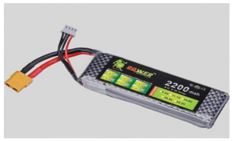
5.6 Battery
The boat is equipped with a LiPo battery (11.1 v, 2200 mAh) to power the Raspberry pi and the motors as shown in Figure 13.
Figure 13. A Lipo battary used in automated boat
In this research, the proposed algorithm is run twelve times. Then the evaluation is based on the following terms:
• Minimum Path Length (Min. length): This value describes the minimum path length obtained over the twelve runs; it is measured by centimeter (cm).
$\mathrm{PL}=\mathrm{d}^* \mathrm{n}^* \mathrm{t}$ (5)
where:
d: it is representing the diameter of DC motor (cm) and equal to 0.15 cm.
n: it is representing the number of rotation DC motor in one sec(rpm/s) and equal to 31 rpm/s.
t: it is representing the time taken of boat from start point to target (sec).
• Average Path Length (Ava. PL): This value describes the average path length over the twelve runs, which is calculated as follows:
Ava. $P L=\frac{\sum_m^i L i}{m}$ (6)
where, Li is the best path length found at an ith run. m is the number of runs; it is measured by centimeter (cm).
• Standard deviation (SD): This metric describes the variance among the twelve runs based on the best path length of each run; it is measured by centimeter (cm).
$\mathrm{S} D=|A v a . P L-P L|$ (7)
The evaluation scenario and analysis experiments of the proposed A* algorithm with PID controller is test by using the proposed system as show in Figure 14 (a) proposed system and (b) system interfacing.
(a)
(b)
Figure 14. (a) Proposed system and (b) interfacing system using fritzing
Figure 15. Proposed environment
After that, the program was uploaded to the raspberry pi 4, the program was write using python 3.10. the evaluation scenario is modelled with the following specifications:
• Static environment with 3 obstacles each obstacle has different size and shapes
• Five cases have been implemented. Each case represents one starting point and one target point as shown in Figure 14. Ten runs are made for each case.
• A* algorithm and modified A* algorithm with PID controller is applied to the proposed environment shown in Figure 15.
The planning environment is a (240 cm×110 cm). The starting point is (X1,Y1) and the target point is (X2,Y2). Figure 16 shows the dimensions of the environment used in this paper.
Figure 16. Dimensions of proposed environment
If we take the first case (start point (105,28), goal point (25,175)), we can note that the path length using the traditional A* algorithm is 261 cm, while the path length using improved algorithm A* with PID controller is 220.5 cm, which indicates an improving in the performance of A* with PID controller.
On the other hand, the results show that for the same case 1, the average path length using A* algorithm is 21.75 cm, while the average path length using A* with PID controller is 18.37 cm, representing a significant. Improvement. A* with PID controller is very close to the shortest path, unlike the normal A* algorithm which was far from the shortest path. Table 3 compares the standard A* algorithm and the improved algorithm A* with PID controller, and also Figure 17 shows a lower standard deviation (SD) in the improved algorithm A* with PID controller. Also, Figure 18 shows comparison for proposed environment between the path length and time for A* without PID controller and A* algorithm with PID controller.
Figure 17. Comparison the standard deviation (SD) for each case of standard and improved A* algorithms
(a)
(b)
Figure 18. (a) Comparison for proposed environment between the path length and time using A* without PID controller and (b) shows path length and time is small for A* algorithm with PID controller
Table 3. Comparison A* without PID controller and A* with PID controller for proposed environment
|
A* Algorithm Without PID Controller |
A* Algorithm with PID Controller |
|||||||||||
|
Cases |
Start Point |
Goal Point |
Path Length (cm) |
Time Taken (sec) |
Average Length (cm) |
Standard Deviation (cm) |
Start Point |
Goal Point |
Path Length (cm) |
Time Taken (sec) |
Average Length (cm) |
Standard Deviation (cm) |
|
1 |
(105,28) |
(25,175) |
261 |
58 |
21.75 |
239.25 |
(105,28) |
(25,175) |
220.5 |
49 |
18.37 |
202.12 |
|
2 |
(15,45) |
(85,203) |
144 |
32 |
12 |
1323 |
(15,45) |
(85,203) |
127.35 |
28.3 |
10.61 |
116.73 |
|
3 |
(72,232) |
(61,33) |
97.2 |
21.6 |
8.1 |
89.1 |
(72,232) |
(61,33) |
85.5 |
19 |
7.12 |
78.375 |
|
4 |
(112,147) |
(89,42) |
86.85 |
19.3 |
7.23 |
79.613 |
(112,147) |
(89,42) |
78.3 |
17.4 |
6.52 |
71.775 |
|
5 |
(12,97) |
(25,175) |
82.8 |
18.4 |
6.9 |
75.9 |
(12,97) |
(25,175) |
70.65 |
15.7 |
5.88 |
64.763 |
According to a comparison of 12 runs and 250 iterations, the improved A* algorithm with PID controller search results are much improved regarding average path length. However, the A star algorithm has some limitations, especially when it comes to dynamic environments where obstacles may move or change position. Additionally, the A star algorithm assumes a perfect knowledge of the environment and its obstacles, which may not always be available. In summary, Real Time Path Planning and static obstacles avoidance in known environments using the A star algorithm is a powerful tool for many applications, but its limitations should be taken into consideration when designing and implementing solutions.
Acknowledgments for Real Time Path Planning and static obstacles avoidance in known environments using the A star algorithm could include:
The developers and researchers who created and optimized the A star algorithm for path planning and obstacle avoidance.
The creators of the software and tools used to implement the algorithm, such as programming languages and libraries. The individuals or organizations who provided the data and maps used in testing and evaluating the algorithm's performance. The communities of researchers and practitioners who have contributed to the field of robotics and autonomous vehicles, and who have advanced the state of the art in path planning and obstacle avoidance. The teachers and educators who have shared their knowledge and expertise with others, helping to train the next generation of robotics and AI professionals.
[1] Åström, K.J., Hägglund, T. (1995). PID Controllers: Theory, Design, and Tuning. ISA - The Instrumentation, Systems and Automation Society.
[2] Brooks, R. (1986). A robust layered control system for a mobile robot. IEEE Journal on Robotics and Automation, 2(1): 14-23. https://doi.org/10.1109/JRA.1986.1087032
[3] Babunski, D., Berisha, J., Zaev, E., Bajrami, X. (2020). Application of fuzzy logic and PID controller for mobile robot navigation. In 2020 9th Mediterranean Conference on Embedded Computing (MECO), Budva, Montenegro, pp. 1-4. https://doi.org/10.1109/MECO49872.2020.9134317
[4] Elfes, A. (1989). Using occupancy grids for mobile robot perception and navigation. Computer, 22(6): 46-57. https://doi.org/10.1109/2.30720
[5] He, R., Prentice, S., Roy, N. (2008). Planning in information space for a quadrotor helicopter in a GPS-denied environment. In 2008 IEEE International conference on Robotics and Automation, Pasadena, CA, USA, pp. 1814-1820. https://doi.org/10.1109/ROBOT.2008.4543471
[6] Huang, C., Lan, Y., Liu, Y., Zhou, W., Pei, H., Yang, L., Cheng, Y., Hao, Y., Peng, Y. (2018). A new dynamic path planning approach for unmanned aerial vehicles. Complexity, 2018: 1-17. https://doi.org/10.1155/2018/8420294
[7] Ozkan, M.F., Carrillo, L.R.G., King, S.A. (2019). Rescue boat path planning in flooded urban environments. In 2019 IEEE International Symposium on Measurement and Control in Robotics (ISMCR), Houston, TX, USA, pp. B2-2. https://doi.org/10.1109/ISMCR47492.2019.8955663
[8] Li, J., Zhang, J. (2021). Global path planning of unmanned boat based on improved ant colony algorithm. In 2021 4th International Conference on Electron Device and Mechanical Engineering (ICEDME), Guangzhou, China, pp. 176-179. https://doi.org/10.1109/ICEDME52809.2021.00045
[9] Vagale, A., Oucheikh, R., Bye, R.T., Osen, O.L., Fossen, T.I. (2021). Path planning and collision avoidance for autonomous surface vehicles I: A review. Journal of Marine Science and Technology, 26: 1292-1306. https://doi.org/10.1007/s00773-020-00787-6
[10] Xiao, X., Dufek, J., Woodbury, T., Murphy, R. (2017). UAV assisted USV visual navigation for marine mass casualty incident response. In 2017 IEEE/RSJ International Conference on Intelligent Robots and Systems (IROS), Vancouver, BC, Canada, pp. 6105-6110. https://doi.org/10.1109/IROS.2017.8206510
[11] Zhang, L., Li, Y. (2021). Mobile robot path planning algorithm based on improved a star. Journal of Physics: Conference Series, 1848(1): 012013. https://doi.org/10.1088/1742-6596/1848/1/012013
[12] Cummings, M.L., Marquez, J.J., Roy, N. (2012). Human-automated path planning optimization and decision support. International Journal of Human-Computer Studies, 70(2): 116-128. https://doi.org/10.1016/j.ijhcs.2011.10.001
[13] Shihab, B.S., Abdullah, H.N., Hassnawi, L.A. (2022). Improved artificial bee colony algorithm-based path planning of unmanned aerial vehicle using late acceptance hill climbing. International Journal of Intelligent Engineering & Systems, 15(6): 431-442. https://doi.org/10.22266/ijies2022.1231.39
[14] Sotnezov, R.M. (2009). Genetic algorithms for problems of logical data analysis in discrete optimization and image recognition. Pattern Recognition and Image Analysis, 19: 469-477. https://doi.org/10.1134/S1054661809030122
[15] Yan, B., Chen, T., Zhu, X., Yue, Y., Xu, B., Shi, K. (2020). A comprehensive survey and analysis on path planning algorithms and heuristic functions. In: Arai, K., Kapoor, S., Bhatia, R. (eds) Intelligent Computing. SAI 2020. Advances in Intelligent Systems and Computing, vol 1228. Springer, Cham. https://doi.org/10.1007/978-3-030-52249-0_39
[16] Wang, Q., Shi, R., Zhang, Q., Yang, X. (2013). Optimal path selection of slow traffic based on GIS network analysis. Journal of Xi’an University of Architecture & Technology, 45(5): 668-674.
[17] Duchoň, F., Babinec, A., Kajan, M., Beňo, P., Florek, M., Fico, T., Jurišica, L. (2014). Path planning with modified a star algorithm for a mobile robot. Procedia Engineering, 96: 59-69. https://doi.org/10.1016/j.proeng.2014.12.098
[18] Dechter, R., Pearl, J. (1985). Generalized best-first search strategies and the optimality of A. Journal of the ACM (JACM), 32(3): 505-536. https://doi.org/10.1145/3828.3830
[19] Abdulameer, A., Sulaiman, M., Aras, M.S.M., Saleem, D. (2016). Tuning methods of PID controller for DC motor speed control. Indonesian Journal of Electrical Engineering and Computer Science, 3(2): 343-349. https://doi.org/10.11591/ijeecs.v3.i2.pp343-349
[20] Phillips, C.L., Harbor, R.D. (1999). Feedback Control Systems. Prentice-Hall, Inc.
[21] Franklin, G.F., Powell, J.D., Emami-Naeini, A., Powell, J.D. (2002). Feedback Control of Dynamic Systems (Vol. 4). Upper Saddle River: Prentice Hall.
[22] Shahrubudin, N., Lee, T.C., Ramlan, R. (2019). An overview on 3D printing technology: Technological, materials, and applications. Procedia Manufacturing, 35: 1286-1296. https://doi.org/10.1016/j.promfg.2019.06.089