Zine Eddine Meguetta![]()
© 2023 IIETA. This article is published by IIETA and is licensed under the CC BY 4.0 license (http://creativecommons.org/licenses/by/4.0/).
OPEN ACCESS
The design of autopilots is often enabled by simulating the behavior of the aircraft when it is steered by these systems. The automatic pilot of an airplane consists of relieving the workload of the crew by allowing it to display an altitude, speed and/or heading instruction and letting the control system manage the trajectory to reach this instruction. The autopilot uses control laws to compare the pilot's flight parameters with the predetermined instructions, then adjusts the control system accordingly. These control laws are parametrized as a function of the stability and precision performances to be respected. The objective of our proposed approach is to demonstrate the usage of Model-Free Control (MFC) using an intelligent controller to check the autopilots altitude based on retention of the aircrafts attitude. The proposed MFC approach is applied in the aircraft system and numerical results have presented good performances in terms that the autopilot altitude regulation error using the MFC controller is more better than the error used by the PID controller.
model-free control MFC, longitudinal aircraft, intelligent controller, PID controller, autopilot altitude
Today, autopilot mechanisms have become very important to ensure safe, long civilian flights for more than 16 hours [1-4]. The system allows the crew of the aircraft to lighten their workload when busy and to assist them in their maneuvers using internal control laws.
System control, and more specifically control and regulation allow a user to ensure that a system is converging to the setpoint it is providing. This discipline has grown exponentially in the age of automation. Remarkable players in this growth are Proportional integrator derivative’s or PID correctors which are essential for any automation specialist, they display their strength very quickly and have established themselves as the easiest way to control a system efficiently. These correctors have countless well-known uses which are within everyone's reach. However, despite this their precision remains low and their configuration complex due to the number of gains requiring adjustment. Since 2007, the Model Free Control (MFC) has been involved in the field of control such as [5-11], which has in the past allowed users to set up correctors without knowing first the dynamic behavior of a certain system. We can address the problem of our research work in this question: Can the MFC allow to subdue/subjugate the behavior of an aircraft on the vertical plane in a simple way? Is it more efficient than the current standard means?
The MFC is associated with a so-called "intelligent" PID corrector because it is characterized by an algebraic estimator to ensure precision. Easier to use and more accurate than traditional PID correctors, this method deserves attention.
In recent years, a great deal of research and studies have been carried out in regards to the development of design systems for autonomous driving (cars, piloting aircraft, etc.) to converge towards reliable performance for the control/command of the dependable vehicle [12-15], and ensure functional solutions in limited driving conditions [15-17]. The PID corrector is a control system that improves the performance of a regulation process. This is the most used in industry regulators where its correction qualities apply to multiple physical quantities.
There are many disadvantages to using different types of PID classical correctors. For instance, the proportional corrector (P) does not independently adjust the speed, the precision, and the margins of stability and among its disadvantages is the risk of instability. The advantage of the Proportional Integrator corrector (PI) is its ability to make the static error zero, but the system is sometimes slow in a closed loop. Proportional derivative (PD) improves stability, speed and the sensitivity of the system to noise. To prevent this, we introduced a bass-pass filter as classical PID has the drawback of difficulties in adjusting parameters.
We used the MFC as it retains the advantages of classical PID without having serious drawbacks. In 2013, Fliess and Join [8] propose to compare regulation by classic continuous and discrete PID with the MFC in the case of a system which had different characteristics in two scenarios. MFC does not require knowledge of the mathematical model of the system [8]. Menhour et al. [16] used a MFC approach leading to “intelligent” controllers. The longitudinal and lateral motions of a Peugeot 406 experimental car were used. This MFC approach associated with the intelligent corrector has had several concrete successes; a comprehensive list, at least until early 2018 in the following bibliographies [8, 10, 11, 18, 19]. In addition, this method is easy to implement to solve various research problems; fault tolerance control is a common subject in the automation field. The growing importance of artificial intelligence and learning particularly through neural networks has naturally been grafted onto the MFC. We are interested in researching within the field of control and in particular correction using the MFC approach associated with an intelligent PID corrector to improve performance of the systems set by the designer in the specifications. A model-free controller with an observer applied in real-time to a 3-DOF helicopter is used by Boubakir et al. [7].
An approach of a model-free controller with an observer is presented for a nonlinear dynamic system Multi Input Multi Output (MIMO) in continuous time. The proposed MFC law consists of: a linear control term used to specify the dynamics of the system in a closed loop and the second part is added to compensate the uncertainties of the dynamic system and external disturbances. The suggested control approach is applied in real-time to a 3-DOF helicopter and experimental results present good performances of the proposed approach MFC.
In the thesis of Bekcheva [6], she studied and differentiated flat systems and the application of the model without control systems whose dynamics and environment were not modeled. This summary focuses on a section of the second part, where the author presents the application of the model without control in a four drone. She first explains the nonlinear model of the drone that is operating in the simulations and then returns to the model without control by developing the waterfall approach. Finally, this approach is validated through several simulations involving unknown disturbances, wind whose amplitude varies over time and variations in mass. In her thesis, she studied design controllers that avoided system identification procedures of the quadrotor while remaining robust in the face of the endogenous (control performances are independent of any change in mass, of inertia, gyroscopic or aerodynamic effects) and exogenous disturbances (wind, measurement noise). Its purpose is based on the cascade structure of a quadrotor, it divides the system into subsystems of position and attitude each controlled by an independent controller with no second order dynamics model. It then gives convincing results on the practical stability of the proposed control design.
Finally, it validates its control approach in three realistic scenarios: in the presence of unknown measurement noise with disturbances due to wind and unknown mass variations over time. The author uses MFC to control the “horizontal elasticity” of a Cloud Computing system [6]. When compared to the commercial “Auto Scaling” algorithms, their feasibility approach performs better, even with sharp workload fluctuations. The authors tested this approach on the Amazon Web Services (AWS) public cloud.
The objective of this research work is the use intelligent model-free control to check the autopilot altitude aircraft. In the first section of this paper, the theoretical bases of MFC control and longitudinal control of an aircraft will be presented. The second section deals with the tests, which lead to the selection of the architecture of the autopilot used during the simulations. In conclusion the third section illustrates the results obtained.
2.1 Principal MFC for SISO system
We restrict SISO systems, characterized by a single input u and a single output y. Model-Free Control (MFC) allows modeling of the system with an ultra-local model of the type [20-23]:
$y^v=F+\alpha u$ (1)
Such as:
y is the output of the system.
F is an estimate of the unknown components of the system as well as of the potential disturbances that affect it.
α is a dimensionless factor with the sole objective of placing all the terms of the formula in the same order of magnitude physical size.
u is the input of the system.
2.1.1 Intelligent PID controller
When considering the case where v is equal to 2 in the previous ultra-local formulation, we can introduce the intelligent PID controller delivering the following control:
$u=\frac{\ddot{y}^*-F+K_p e+K_I \int e+K_D \dot{e}}{\alpha}$ (2)
Such as:
$y^*$ is the setpoint.
$K_p, K_I, K_D$ are the gains of the PID controller.
The error is:
$e=y^*-y$ (3)
The error e is obtained by comparing the output of the system with the reference trajectory.
In the case where v is equal to 1, we find two different intelligent controllers:
Intelligent PI controllers:
$u=\frac{\ddot{y}^*-F+K_p e+K_I \int e}{\alpha}$ (4)
Intelligent P controllers:
$u=\frac{\ddot{y}^*-F+K_p e}{\alpha}$ (5)
These controllers are therefore standard PID controllers into which a term is also injected which makes it possible to estimate the fluctuations of the output and which improves the accuracy of the controller.
From Eq. (1), F is a continuously updated value that represents the overall time-varying dynamics of the system, and it could be approximately estimated using the information from the control signal u and $y^v$ [11, 20].
In the reference [11], the efficiency and robustness against noise are demonstrated by three illustrative examples and their simulation results.
Recent algebraic parameter identification techniques presented by Fliess and Sira-Ramirez [11], and Sira-Ramírez et al. [21], and Riachy's trick permit to avoid tedious numerical derivations of the output signal y [22].
Good robustness with respect to corrupting noises is ensured via a new noise understanding. The gain tuning is straightforward.
2.1.2 Estimation of F
Model-Free Control (MFC) involves a term made up of the unknown parts of the system as well as the disturbances to which it is subjected. A suitable approximate estimation of F in Eq. (1) boils down, therefore, to the estimation of the constant parameter $\phi$ in the following equation $y^v=\phi+\alpha u$ if it can be achieved during a sufficiently ‘small’ time interval. The objective is therefore to discretize the time domain over sufficiently small intervals.
Analogous estimations of F may be carried on via the intelligent controllers (Eq. (2), Eq. (4), Eq. (5)).
In order to encompass all the previous equations, where F is estimated, the study of the physical model of the studied system where the classic rules of operational calculus are utilized by the studies [24, 25], gives us an equation in the frequency domain of the type:
$L_1(S) Z_1+L_2(S) Z_2=\frac{\phi}{S}+I(S)$ (6)
With:
L1 and L2 are polynomials of Laurent.
I a polynomial associated with the initial conditions.
$\phi$ the constant to be determined.
Finally, the corresponding formula in the time domain is deduced with two rules in mind:
The negative powers of s correspond to integrations in time.
A derivation according to s corresponds to a multiplication by (-t) in time. We then obtain the ultra-local estimate of F:
$\phi=-\frac{6}{L^3} \int_{t-L}^t((L-2 \sigma) y(\sigma)+\alpha \sigma(L-\sigma) u(\sigma)) d \sigma$ (7)
With L a small chosen parameter, depending on the sampling period and the noise applied to the system.
2.2 Principal MFC for MIMO system
Several works and authors deal with the adaptation of MFC to MIMO systems, therefore there are several methods. Among them, we find in the study [5], the aim of this work is to design a single corrector whose inputs are the respective errors of all the outputs of the system and whose outputs are all the commands of the system.
The two other methods allow the MIMO system to be built with multiple SISO systems using cascade control, as shown by the studies [6, 7], or parallel control dealt by Fliess and Join [8].
Based on the knowledge principle of model-free control design for SISO system, the work described in the study [5] propose a partial model-free control design method for the ultra-local system; firstly, the derivative of y(t) is estimated by the low-pass filter, then, the dynamics of the system F(t) is obtained from the derivative estimation and the control input, with the model-free design.
The tracking control problem of the complex nonlinear MIMO dynamic system has been transformed from a partial control to a decomposed linear system [23]; the next step is to design the control law.
For simplicity, we will use cascade and parallel control to make use of our knowledge and principles of SISO systems, the proposed enslavement is inspired by both the parallel and cascade schemes discussed above.
3.1. Autopilot architecture
Designing a complete autopilot involves synthesizing multiple controllers. Indeed, the structure of an autopilot includes several control loops. The Figure 1 illustrates the different control loops that can be found in a modern airplane. A first control loop, called internal loop, makes it possible to improve the natural flight qualities of the aircraft as well as its maneuverability. This control loop generally consists of a Stability Augmentation System (SAS) and a Controllability Augmentation System (CAS) [23]. A second control loop, called external loop, allows the command of the pilot or the flight management system to be translated into terms of control for the internal loop. It is also divided into several sub-loops depending on the modes that the autopilot has. Here we list some of them: vertical speed hold mode, altitude hold mode, heading capture mode, speed hold mode. In this work, we are interested in the altitude hold mode.
SAS are generally designed in accordance with standards relating to the specific modes of the system, namely the angle of attack recall mode, the phugoid mode and the propulsion recall mode. These standards relate to the frequency and damping of modes. We will not go so far as to generate these specifications; we will accept a model already designed. However, we can define time specifications concerning the CAS and the autopilot.
Figure 1. Positions of SAS and CAS in the control system of an aircraft
3.2 Model validation
In order to simulate the behavior of the aircraft when controlled with a MFC controller, it is first necessary to verify that the modules used in the simulation are valid. These modules concern the controller as well as the aircraft. The architecture of the autopilot, that is to say the assembly of these modules, was also verified. Validation focuses on the error between actual and desired altitude.
The modules concerned control the aircraft using two elements: algorithm MFC control and Simulink diagram.
The purpose of section 3 is to present the Algorithm MFC control and Simulink diagram where two scenarios are shown; the algorithm was validated by simulating two scenarios presented. Each scenario applies the MFC control on a different system.
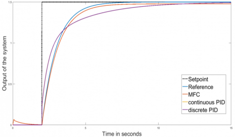
Figure 2 compares the reference trajectory with the setpoint. The MFC control algorithm simulates the behavior of the system using a loop and a dedicated MFC function.
The parameters of the model MFC are the same in both scenarios; the first one, simple reference trajectory and second scenario is complex reference trajectory. The results are shown in Figures 3 and 4.
3.2.1 Algorithm MFC control
Firstly, to control SISO type systems we created a function to calculate the control of MFC while knowing the setpoint applied as well as the parameters chosen: the integration time L, the factor a and the gains P, D, and I. In fact, in this algorithm, the MFC function is associated with an intelligent proportional corrector to simplify the simulations and not to consider any integral and derivative gains. We take the case of v=1.
In the algorithm for calculating the MFC control, the reference path is obtained by applying the filter to the setpoint as:
$H(s)=\frac{1}{1+s}$ (8)
Figure 2 compares the reference trajectory with the setpoint. A zoom on the graphs of Figure 2 is also given. The error e is obtained by comparing the output of the system with the reference trajectory. The MFC control algorithm simulates the behavior of the system using a loop and a dedicated MFC function.
The objective of this section of the research work is to control the system under study in such a way that it follows the behavior of a reference model. To do this, a reference trajectory is calculated from the input control: this is the trajectory that the reference model virtually follows if stimulated by the control. Thus, to obtain the reference trajectory necessary for the calculation of the model-free control, a reference model must be defined.
Figure 2 shows the different responses of the MFC output, discrete PID and continuous PID for first order system: $\frac{1}{1+s}$.
From Figure 2: We remark that that control by MFC is better than control by PID.
This algorithm was validated by simulating two scenarios presented by Fliess and Join [8] and comparing the results with those of the article. Each scenario applies the MFC control on a different system:
In the first scenario, we have:
$H(s)=\frac{(s+2)^2}{(s+1)^2}$ (9)
For the second scenario, we have:
$H(s)=\frac{(s+2)^2}{(s+2.2)^2}$ (10)
Figure 2. Comparison of the setpoint and different control responses of the system
The parameters of the model MFC are the same in both scenarios. The results are shown in Figures 3 and 4.
The noise simulation is not strictly similar in the two scenarios because the authors do not specify all the specifications concerning the generation of the disturbances. No precise measurement is possible because the authors results are only available in the form of graphs, however it is noted that the respective simulations of the scenarios are strongly similar. This similarity is observed in both scenarios, which allows us at this point to consider the model offered by our computation algorithm MFC function valid.
Figure 3. Comparison of simulations for Scenario 1
Figure 4. Comparison of simulations for Scenario 2
The same results presented in the work [8] were found using our simulation algorithm. As the authors of the latter do not give the disturbance values for the two scenarios, we simulated without the presence of disturbance.
Regarding our simulation algorithm for SISO system, we coded the theoretical part of the MFC SISO approach, that is to say, the Eq. (2), Eq. (3), and Eq. (7).
The used aircraft physical model is illustrated in Figure 5.
Figure 5. Aircraft physical model
The aircraft chosen is similar to a Dassault Mirage III, with the following parameters and at the given flight conditions:
Aircraft mass $m=8500 \mathrm{Kg}$, Altitude $z=3052$m, Mach number $M=0.8$, Air density $\rho=0.9 \mathrm{Kg} \cdot \mathrm{m}^{-3}$, variation of lift regarding deflection of the elevator $C_{Z M}=1.1$, variation of lift regarding variation of angle of attack $C_{Z \alpha}=2.66$, variation of pitch moment regarding variation pitch velocity $C_{m q}=-0.68$, induced drag coefficient $k=0.22$, parasite drag coefficient $C_{x 0}=0.015$, moment of inertia $I_Y=59691 \mathrm{~kg} \cdot \mathrm{m}^{2}$, reference surface $S=34$m2, reference length $l=5.24 \mathrm{~m}$, acceleration due to gravity $g=9.81 \mathrm{~m} \cdot \mathrm{s}^{-2}$.
Under such conditions, the point of equilibrium is the following:
Total drag coefficient $C_{\text {xe }}=0.0163$.
Other important notations are the following:
Thrust F, total Lift coefficient Cz, total drag coefficient Cx, total pitch moment coefficient Cm.
The previous coefficients synthesize the several components of force or moment as shown in the following equations:
$C_z=C_{z \alpha}\left(\alpha-\alpha_0\right)+C_{z m} \delta m$ (11)
$C_m=C_{m 0}+C_{m \alpha}\left(\alpha-\alpha_0\right)+C_{m m} \delta m+C_{m q} \frac{l q}{V}$ (12)
$C_x=C_{x 0}+K C_z^2$ (13)
Longitudinal flight involves the following angles: The attitude $\theta$, The slope $\gamma$, The angle of attack $\alpha$.
The following relation in the case of pure longitudinal flight was noticed:
$\theta=\alpha+\gamma$
By applying the fundamental principle of dynamics and the fundamental principle of kinematics in the benchmarks presented above, we can obtain several equations relating the state variables to each other.
Equations in the aerodynamic landmark:
Equation of propulsion; projection of forces on the axis x:
$m \dot{V}=-\frac{1}{2} \rho S V^2 C_X+F \cos (\alpha)-m g \sin (\gamma)$ (14)
Equation of sustenance; projection of forces on the axis z:
$-m V \dot{\gamma}=-\frac{1}{2} \rho S V^2 C_z-F \sin (\alpha)-m g \cos (\gamma)$ (15)
Equation of Moment; around the axis y:
$I_Y \dot{q}=\frac{1}{2} \rho S V^2 l C_m$ (16)
Kinematic Eq. (1); attitude:
$\dot{\theta}=q=\frac{d \alpha}{d t}+\frac{d \gamma}{d t}$ (17)
Kinematic Eq. (2); altitude:
$h=V \sin (\gamma)$ (18)
Matrices A and B are obtained with the linearization method presented in the next section, in the case of longitudinal flight and with the following further assumptions:
To simplify the study of the behavior of the airplane, we can consider that the airplane is in pure longitudinal flight, that the sideslip $\beta$, the speeds of rotation in yaw r and in roll p and inclination $\phi$ are zero. These assumptions make it possible to reduce the number of state variables to 6: Speed V, The angle of attack $\alpha$, The slope $\gamma$, The altitude h, The pitch rotation speed q, attitude $\theta$.
Considering that the aircraft is in flight, pure longitudinal amounts in estimating the lateral state variables ($\beta, p, r$ and $\varphi$) have a negligible impact on the longitudinal state variables ($V, \alpha, \gamma, h, \theta, q$), that is to say that the longitudinal behavior of the aircraft will be almost the same whether, for example, it is in a turn or not. This approximation has been observed thanks to the numerous tests that have taken place throughout the history of aviation.
This manipulation then allows us to calculate the derivatives of the variables between them, by taking the value of the equilibrium state variables, this is the term $\left(\frac{\partial f}{\partial x}\right)_e$.
From now on, the state variables will denote the deviation from the equilibrium value, except for the speed, which will be dimensionless, that is to say:
$V=\frac{\delta V}{V_e}$ (19)
where, $\gamma=\delta \gamma, \alpha=\delta \alpha, q=\delta q, z=\delta z$.
The state space is used to represent a linear system, whether MIMO or SISO using matrices:
$\dot{X}=A X+B U$ (20)
Meanwhile: A is the state matrix or evolution matrix, B is dynamic matrix, u the command vector, X the state vector. The state vector is composed of state variables, so in the case of longitudinal flight we have:
$X=\left[\begin{array}{l}V \\ \gamma \\ \alpha \\ q \\ \theta \\ z\end{array}\right]$
The control vector is composed of the controls, so in the case of longitudinal flight, with $\delta m$ the elevator control and $\delta \tau$ the throttle control, we have:
$u=\left[\begin{array}{l}\delta m \\ \delta \tau\end{array}\right]$
Matrices A and B are obtained with the linearization method presented in the previous chapter. In the case of longitudinal flight, we have:
$A=\left[\begin{array}{llllll}\left(\frac{\partial V}{\partial V}\right)_e & \left(\frac{\partial V}{\partial \gamma}\right)_e & \left(\frac{\partial V}{\partial \alpha}\right)_e & \left(\frac{\partial V}{\partial q}\right)_e & \left(\frac{\partial V}{\partial \theta}\right)_e & \left(\frac{\partial V}{\partial z}\right)_e \\ \left(\frac{\partial \gamma}{\partial V}\right)_e & \left(\frac{\partial \gamma}{\partial \gamma}\right)_e & \left(\frac{\partial \gamma}{\partial \alpha}\right)_e & \left(\frac{\partial \gamma}{\partial q}\right)_e & \left(\frac{\partial \gamma}{\partial \theta}\right)_e & \left(\frac{\partial \gamma}{\partial z}\right)_e \\ \left(\frac{\partial \alpha}{\partial V}\right)_e & \left(\frac{\partial \alpha}{\partial \gamma}\right)_e & \left(\frac{\partial \alpha}{\partial \alpha}\right)_e & \left(\frac{\partial \alpha}{\partial q}\right)_e & \left(\frac{\partial \alpha}{\partial \theta}\right)_e & \left(\frac{\partial \alpha}{\partial z}\right)_e \\ \left(\frac{\partial q}{\partial V}\right)_e & \left(\frac{\partial q}{\partial \gamma}\right)_e & \left(\frac{\partial q}{\partial \alpha}\right)_e & \left(\frac{\partial q}{\partial q}\right)_e & \left(\frac{\partial q}{\partial \theta}\right)_e & \left(\frac{\partial q}{\partial z}\right)_e \\ \left(\frac{\partial \theta}{\partial V}\right)_e & \left(\frac{\partial \theta}{\partial \gamma}\right)_e & \left(\frac{\partial \theta}{\partial \alpha}\right)_e & \left(\frac{\partial \theta}{\partial q}\right)_e & \left(\frac{\partial \theta}{\partial \theta}\right)_e & \left(\frac{\partial \theta}{\partial z}\right)_e \\ \left(\frac{\partial z}{\partial V}\right)_e & \left(\frac{\partial z}{\partial \gamma}\right)_e & \left(\frac{\partial z}{\partial \alpha}\right)_e & \left(\frac{\partial z}{\partial q}\right)_e & \left(\frac{\partial z}{\partial \theta}\right)_e & \left(\frac{\partial z}{\partial z}\right)_e\end{array}\right]$
The analytical expression of the matrix A is given by:
$\begin{aligned} & A= {\left[\begin{array}{cccccc}-\frac{\rho V_e S C_{x e}}{m} & -\frac{g \cos \left(\alpha_e\right)}{V_e} & -\frac{F_e \sin \left(\alpha_e\right)+\frac{1}{2} \rho V_e^2 S C_{x \alpha}}{m V_e} & 0 & 0 & 0 \\ \frac{2 g}{V_e} & 0 & \frac{F_e \cos \left(\alpha_e\right)+\frac{1}{2} \rho S V_e^2 C_{z \alpha}}{m V_e} & 0 & 0 & 0 \\ -\frac{2 g}{V_e} & 0 & -\frac{F_e \cos \left(\alpha_e\right)+\frac{1}{2} \rho S V_e^2 C_{z \alpha}}{m V_e} & 1 & 0 & 0 \\ 0 & 0 & \frac{\frac{1}{2} \rho S V_e^2 C_{m \alpha}}{I_y} & \frac{\frac{1}{2} \rho S V_e^2 l^2 C_{m q}}{I_Y V_e} & 0 & 0 \\ 0 & 0 & 0 & 1 & 0 & 0 \\ 0 & V e & 0 & 0 & 0 & 0\end{array}\right]} \\ & \end{aligned}$
The matrix B is defined as:
$B=\left[\begin{array}{ll}\left(\frac{\partial V}{\partial \delta m}\right)_e & \left(\frac{\partial V}{\partial \delta \tau}\right)_e \\ \left(\frac{\partial \gamma}{\partial \delta m}\right)_e & \left(\frac{\partial \gamma}{\partial \delta \tau}\right)_e \\ \left(\frac{\partial \alpha}{\partial \delta m}\right)_e & \left(\frac{\partial \alpha}{\partial \delta \tau}\right)_e \\ \left(\frac{\partial q}{\partial \delta m}\right)_e & \left(\frac{\partial q}{\partial \delta \tau}\right)_e \\ \left(\frac{\partial \theta}{\partial \delta m}\right)_e & \left(\frac{\partial \theta}{\partial \delta \tau}\right)_e \\ \left(\frac{\partial z}{\partial \delta m}\right)_e & \left(\frac{\partial z}{\partial \delta \tau}\right)_e\end{array}\right]=\left[\begin{array}{ll} 0 & \frac{F_\tau \sin \left(\alpha_e\right)}{m V_e} \\\frac{\frac{1}{2} \rho S V_e C_{z m}}{m} & 0 \\ -\frac{\frac{1}{2} \rho V_e S C_{z m}}{m} & 0 \\ \frac{\frac{1}{2} \rho V_e^2 S l C_{m m}}{I_Y} & -\frac{\frac{1}{2} \rho S V_e^2 l C_{m m}}{I_Y} \\ 0 & 0 \\ 0 & 0\end{array}\right]$
To specify the outputs concerned, which are placed in the vector Y, one also indicates the matrices C and D such as:
$Y=C X+D U$ (21)
where,
$C=\left[\begin{array}{llllll}1 & 0 & 0 & 0 & 0 & 0 \\ 0 & 1 & 0 & 0 & 0 & 0 \\ 0 & 0 & 1 & 0 & 0 & 0 \\ 0 & 0 & 0 & 1 & 0 & 0 \\ 0 & 0 & 0 & 0 & 1 & 0 \\ 0 & 0 & 0 & 0 & 0 & 1\end{array}\right], D=\left[\begin{array}{l}0 \\ 0 \\ 0 \\ 0 \\ 0 \\ 0\end{array}\right]$
To specify the outputs concerned, which are placed in the vector Y, one also indicates the matrices C and D such as: it can be seen that the aircraft in longitudinal flight is a system with several inputs ($\delta m$ and $\delta \tau$) and we will see later in this article that it can also have several outputs in order to be controlled correctly.
The following algorithm presented in Figure 6 was developed to vary the Mach and flight altitude. We took the neighborhood of the nominal conditions $M=0.8$ and $Z=3048$ meters to obtain the space state matrices.
The simplest model studied is a decoupled model where only the variables evolving notably with the incidence oscillation mode are considered [1, 2]. This made it possible to verify that the results obtained by the basic simulations were correct. The advantage of simulating this system before moving on to a more complex one is that it is easy to build a Simulink diagram around this state space, by analyzing only two variables.
$\left[\begin{array}{c}\dot{\alpha} \\ \dot{q}\end{array}\right]=\left[\begin{array}{cc}-1.266 & 1 \\ -7.4016 & -1.2576\end{array}\right]\left[\begin{array}{c}\alpha \\ q\end{array}\right]+\left[\begin{array}{c}-0.5203 \\ -39.7908\end{array}\right] \delta_m$
Figure 6. Equilibrium point calculation algorithm
The simulations are then run on the complete system, with the 6 state variables; as well as the variable $\theta$ which is obtained by integrating q. The attitude $\theta$ is integrated into the state model for reasons of simplicity, in order to have direct access to it, it should be noted that it is sufficient to add the slope and the incidence to obtain it, if it does not it is not integrated into the article model. First, the throttle $\delta \tau$ is zero, the control then relates to several outputs ($q, \theta$ and $z$) and to a single input $\delta m$.
$\begin{aligned} & {\left[\begin{array}{c}\dot{V} \\ \dot{\gamma} \\ \dot{\alpha} \\ \dot{q} \\ \dot{\theta} \\ \dot{Z}\end{array}\right]=\left[\begin{array}{cccccc}-0.0155 & -0.0373 & -0.0436 & 0 & 0 & 0 \\ 0.074 & 0 & 1.266 & 0 & 0 & 0 \\ -0.074 & 0 & -1.266 & 1 & 0 & 0 \\ 0 & 0 & -7.4016 & -1.2576 & 0 & 0 \\ 0 & 0 & 0 & 1 & 0 & 0 \\ 0 & 262.79 & 0 & 0 & 0 & 0\end{array}\right]\left[\begin{array}{l}V \\ \gamma \\ \alpha \\ q \\ \theta \\ 0\end{array}\right]+} {\left[\begin{array}{c}0.5203 \\ -0.5203 \\ -39.7908 \\ 0 \\ 0\end{array}\right] \delta_m}\end{aligned}$
5.1 Control of aircraft attitude
The first stage of research work consists of controlling attitude using a MFC and a PID controller. The simulation result is shown in the Figure 7.
The Comparison between the characteristics of $\theta_{P I D}$ and $\theta_{M F C}$ is summarized in the Table 1.
According to the characteristics illustrated in Table 1, which illustrate each response of the aircrafts attitude. The Aircraft attitude $\theta_{M F C}$ is selected.
Table 1. Comparison between the characteristics of $\theta_{P I D}$ and $\theta_{M F C}$
|
Characteristics |
$\theta_{P I D}$ |
$\theta_{M F C}$ |
|
Rise Time |
2.4852 |
2.2008 |
|
Settling Time |
4.6268 |
3.9343 |
|
Settling Min |
0.8999 |
0.900 |
|
Settling Max |
0.9998 |
1.000 |
|
Overshoot |
0 |
1.6534e-04 |
|
Peak |
0.998 |
1.000 |
|
Peak Time |
10 |
9.997 |
Figure 7. Step response of the aircraft attitude $\theta$ using MFC controller and PID regulator
5.2 Control of the altitude
The second stage of research work consisted of controlling altitude using throttle control. The state space is then as follows:
$\begin{aligned} & {\left[\begin{array}{c}\dot{V} \\ \dot{\gamma} \\ \dot{\alpha} \\ \dot{q} \\ \dot{\theta} \\ \dot{Z}\end{array}\right]=\left[\begin{array}{cccccc}-0.0155 & -0.0373 & -0.0436 & 0 & 0 & 0 \\ 0.074 & 0 & 1.266 & 0 & 0 & 0 \\ -0.074 & 0 & -1.266 & 1 & 0 & 0 \\ 0 & 0 & -7.4016 & -1.2576 & 0 & 0 \\ 0 & 0 & 0 & 1 & 0 & 0 \\ 0 & 262.79 & 0 & 0 & 0 & 0\end{array}\right]\left[\begin{array}{l}V \\ \gamma \\ \alpha \\ q \\ \theta \\ z\end{array}\right]+} {\left[\begin{array}{cc}0.5203 & 0 \\ -0.5203 & 0 \\ -39.7908 & -39.7908 \\ 0 & 0 \\ 0 & 0\end{array}\right]\left[\begin{array}{l}\delta_m \\ \delta_\tau\end{array}\right]}\end{aligned}$
Our objective:
Figure 8. Functional diagram to control the attitude and altitude of the aircraft
Maintain the aircraft altitude displayed by the pilot because altitude is an important navigation parameter (anti-collision); when the "vertical speed" mode is activated. We controlled altitude z using a MFC and a PID Controller using the functional diagram is illustrated in Figure 8.
With: ZC is the altitude of reference equal 10000 meter $K_\theta$ is gain constant used for simulation. p is the operator of Laplace. Bloc KZ can take two cases of controllers:
Firstly, the gain of MFC approach control and secondly gain of PID (Figures 9 and 10).
A zoom on the error of attitude $\theta$ is given on Figure 9.
Figure 9. Step response of the Altitude using MFC controller and PID regulator and error zoom of the attitude $\theta$
Figure 10. Error of Step response of the Altitude using MFC and PID controller
Table 2. Comparison between the characteristics of $Z_{M F C}$ and $Z_{P I D}$
|
Characteristics |
Altitude $Z_{M F C}$ |
Altitude $Z_{P I D}$ |
|
Rise Time |
185.4359 |
223.6703 |
|
Settling Time |
400.4539 |
558.7572 |
|
Settling Min |
8.9896e+03 |
9.1263e+03 |
|
Settling Max |
9.9837e+03 |
1.0392e+04 |
|
Over shoot |
0 |
2.6483 |
|
Peak |
9.9837e+03 |
1.0392e+04 |
|
Peak Time |
1001 |
451 |
According Figure 10, we see that the MFC response is better than the PID response because the error of step response of the altitude using MFC controller is less that the error of step response of the Altitude using PID controller. In time interval (s): [0.5, 3] we see some oscillations in the transient response after becoming stable and precise in the steady state.
We did not choose the PID response because there is an overshoot in steady state and an error in the 2 states: transient and permanent. The comparison between the characteristics of $Z_{M F C}$ et $Z_{P I D}$ is presented in the Table 2. The longitudinal control of the aircraft is ensured and satisfactory with regard to response time at 5% and lower overshooting.
In this article, a model-free control approach was proposed to control a nonlinear aircraft system. The tracking control problem of this complex nonlinear MIMO dynamic system has been transformed decomposed control.
Based on the proposed model-free control strategy, the control altitude is taken from the aircraft attitude to the control parameters of autopilot. From the study of the simulation, we find the control effects of the model-free control method are quite promising according to control performances; that is to say, satisfactory model with regard to rapid response time and lower overshoot and zero error.
Based on the proposed model-free control approach, the control altitude is taken from the aircraft attitude to the control parameters of autopilot. From the study of the simulation and the comparison results of PID and MFC controller, we find the control effects of the model-free control method are quite promising according to control performances. Simulations have confirmed the benefit of model-free control in the aeronautical field.
In future work, we want to apply this method on a real system, either a quadrotor with 4 DC motors or on a Quanser Aero system. Also, we would like to develop an autopilot for a MIMO System with constraints and uncertain disturbances. This work impacts the field of aircraft control systems, for example, MFC controller can be applied to different levels of the autopilot, that to say, maintaining a given speed.
|
m |
Aircraft mass Kg |
|
Greek Symbols |
|
|
$\alpha$ |
is a dimensionless factor with the sole objective |
|
$\phi$ |
the constant to be determined |
|
$\rho$ |
Air density $\mathrm{Kg} \cdot \mathrm{m}^{-3}$ |
|
$V_e$ |
velocity $m \cdot s^{-1}$ |
|
$F_e$ |
Thrust N |
|
$\alpha_e$ |
Angle of attack rad |
|
Subscripts |
|
|
P |
Proportional-Integral-Derivative |
|
MFC |
Model-Free Control |
[1] Cook, M.V. (2007). Flight Dynamics Principle, second ed. Elsevier-Aaerospace Engineeing Series, USA.
[2] Etkin, B., Reid, L.D. (1995). Dynamics of Flight: Stability and Control. John Wiley & Sons.
[3] Stevens, B.L., Lewis, F.L., Johnson, E.N. (2015). Aircraft Control and Simulation: Dynamics, Controls Design, and Autonomous Systems. John Wiley & Sons.
[4] Yedavalli, R.K. (2020). Flight Dynamics and Control of Aero and Space Vehicles. John Wiley & Sons.
[5] Xin, Y., Qin, Z.C., Wu, W.G., Sun, J.Q. (2017). Partial model-free control of a 2-input and 2-output helicopter system. In Conference Record. 2017 the 9th European Nonlinear Dynamics Conference.
[6] Bekcheva, M. (2019). Flatness-based constrained control and model-free control applications to quadrotors and cloud computing. Doctoral dissertation, Université Paris-Saclay (ComUE). http://www.theses.fr/2019SACLS218.
[7] Boubakir, A., Labiod, S., Boudjema, F., Plestan, F. (2014). Model-free controller with an observer applied in real-time to a 3-DOF helicopter. Turkish Journal of Electrical Engineering and Computer Sciences, 22(6): 1564-1581. https://doi.org/10.3906/elk-1204-54
[8] Fliess, M., Join, C. (2013). Model-free control. International Journal of Control, 86(12): 2228-2252. https://doi.org/10.1080/00207179.2013.810345
[9] Fliess, M., Join, C., Voyant, C. (2018). Prediction bands for solar energy: New short-term time series forecasting techniques. Solar Energy, 166: 519-528. https://doi.org/10.1016/j.solener.2018.03.049
[10] Abouaïssa, H., Hasan, O.A., Join, C., Fliess, M., Defer, D. (2017). Energy saving for building heating via a simple and efficient model-free control design: First steps with computer simulations. In 2017 21st International Conference on System Theory, Control and Computing (ICSTCC), IEEE, pp. 747-752. https://doi.org/10.1109/ICSTCC.2017.8107126
[11] Fliess, M., Sira-Ramirez, H. (2008). Closed-loop parametric identification for continuous-time linear systems via new algebraic techniques. Identification of Continuous-Time Models from Sampled Data, 363-391. https://doi.org/10.1007/978-1-84800-161-9_13
[12] Meguetta, Z.E., Conrard, B., Bayart, M. (2016). Design methodology of a reliable control system using a structural analysis approach. International Journal of Systems Science: Operations & Logistics, 3(3): 129-137. https://doi.org/10.1080/23302674.2015.1039626
[13] Fayyaz, M., Vladimirova, T. (2016). Survey and future directions of fault-tolerant distributed computing on board spacecraft. Advances in Space Research, 58(11): 2352-2375. https://doi.org/10.1016/j.asr.2016.08.017
[14] Lu, K., Xia, Y., Shen, G., Yu, C., Zhou, L., Zhang, L. (2017). Sliding mode control for Mars entry based on extended state observer. Advances in Space Research, 60(9): 2009-2020. https://doi.org/10.1016/j.asr.2017.06.014
[15] Luo, J., Zhou, L., Zhang, B. (2017). Consensus of satellite cluster flight using an energy-matching optimal control method. Advances in Space Research, 60(9): 2047-2059. https://doi.org/10.1016/j.asr.2017.07.013
[16] Menhour, L., d’Andréa-Novel, B., Fliess, M., Gruyer, D., Mounier, H. (2017). An efficient model-free setting for longitudinal and lateral vehicle control: Validation through the interconnected Pro-SiVIC/RTMaps prototyping platform. IEEE Transactions on Intelligent Transportation Systems, 19(2): 461-475. https://doi.org/10.1109/TITS.2017.2699283
[17] Ma, T. (2021). Recursive filtering adaptive neural fault-tolerant control for uncertain multivariable nonlinear systems. European Journal of Control, 59: 274-289. https://doi.org/10.1016/j.ejcon.2020.10.003
[18] Fliess, M., Join, C. (2022). An alternative to proportional‐integral and proportional‐integral‐derivative regulators: Intelligent proportional‐derivative regulators. International Journal of Robust and Nonlinear Control, 32(18): 9512-9524. https://doi.org/10.1002/rnc.5657
[19] Barth, J.M., Condomines, J.P., Bronz, M., Moschetta, J.M., Join, C., Fliess, M. (2020). Model-free control algorithms for micro air vehicles with transitioning flight capabilities. International Journal of Micro Air Vehicles, 12: 1756829320914264. https://doi.org/10.1177/1756829320914264
[20] Fliess, M., Sira-Ramírez, H. (2003). An algebraic framework for linear identification. ESAIM: Control, Optimisation and Calculus of Variations, 9: 151-168. https://doi.org/10.1051/cocv:2003008
[21] Sira-Ramírez, H., Rodríguez, C.G., Romero, J.C., Juárez, A.L. (2014). Algebraic Identification and Estimation Methods in Feedback Control Systems. John Wiley & Sons.
[22] Riachy, S., Fliess, M. (2011). High-order sliding modes and intelligent PID controllers: First steps toward a practical comparison. IFAC Proceedings Volumes, 44(1): 10982-10987. https://doi.org/10.3182/20110828-6-IT-1002.01472
[23] Meguetta, Z.E., Durlin, A., Rahal, M.I., Chaabna, A., Bayart, M. (2021). The different theoretical methods of the MFC approach for a MIMO system. In 2021 9th International Conference on Systems and Control (ICSC), Caen, France, pp. 510-515. https://doi.org/10.1109/ICSC50472.2021.9666678
[24] Mikusinski, J. (1987). Operational Calculus. PWN-Pergamon Press.
[25] Yosida, K. (1984). Operational Calculus. Translated from the Japanese. Springer.