Saad M. Alwash*![]() | Osama Qasim Jumah Al-Thahab
| Osama Qasim Jumah Al-Thahab![]() | Shamam F. Alwash
| Shamam F. Alwash![]()
© 2023 IIETA. This article is published by IIETA and is licensed under the CC BY 4.0 license (http://creativecommons.org/licenses/by/4.0/).
OPEN ACCESS
The paper presents a comprehensive study on modeling a doubly fed induction generator (DFIG) and explores various control strategies for pulse-width modulation (PWM) in back-to-back (B2B) converter techniques. A DFIG is characterized by a wound rotor and three slip-ring induction machines, with the stator winding directly connected to the power grid and the wound rotor interfaced with the grid through a 3-phase AC/DC/AC converter. Typically, the converter connected to the grid is referred to as the grid side converter (GSC), while the converter attached to the rotor's slip-ring circuit is termed the rotor side converter (RSC). This research delineates various PWM-based B2B converter methodologies applied to the DFIG within wind energy turbines, aiming to regulate the RSC for optimal power capture. The study employs MATLAB/SIMULINK for constructing a multi-phase voltage source converter two-level (VSC-2L) model, leveraging different PWM techniques including Sine-PWM, Sinusoidal-PWM with third harmonic injection (THIPWM), and space vector PWM (SVPWM). These techniques are assessed based on total harmonic distortion (THD) using fast Fourier transform (FFT) analysis. The findings indicate that SVPWM offers several advantages, such as ease of digital implementation, lower THD, reduced switching frequency losses, and more efficient utilization of the DC link voltage, thereby enhancing control strategy effectiveness.
SVPWM, SPWM, THIPWM, THD, wind turbine, B2B converter
In recent years, the use of semiconductor-based device drivers has increased. The electronic circuit converter is used as the interface between the wind energy generator and the network for controlling the real and reactive output power. Two primary categories of wind systems are based on the rotor speed control criterion. The first turbine runs at a fixed angular speed known as a Fixed-Speed Wind Turbine (FSWT); the generator's speed varies commonly within 1% of the synchronous speed [1]. In this type, the wind speed is independent without using a power voltage source converter (VSC) interface based on an asynchronous machine. It is simple in structure, but it is not capable of maximum power point according to the variation of the wind speeds and more stress on the mechanical turbine blade. The other type of turbine is capable of adjusting the speed of the rotor, called Variable-Speed Wind energy Turbine (VSWT), and is widely used nowadays [2]. The wind turbine will be able to run at variable speeds to maintain maximum power extraction under different wind speeds with a suitable control electronic converter (full-power converter or partial-power converter). Power electronics in full-rated power converter wind turbines are linked between the stator of the generator and the electrical network. But, in the partial-rated converter, the power voltage converter is linked between the slip-ring rotor and the electric grid [3].
Indeed, all wind turbines utilize synchronous or asynchronous generators, so the most common ones are DFIG and Permanent Magnet Synchronous Generators (PMSG) (WTs). The PMSG machines do not require any added excitation compared with the DFIG [4, 5].
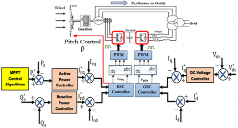
Figure 1. Wind turbine with (DFIG-2L-B2B) converter
The DFIG wind turbine has a partial-power converter (20%–30%) of the generator-rated. The control GSC has two main aims: control of the DC bus to keep a constant voltage and to maintain the ripple in the DC link as small as possible, whereas the RSC regulates generator power (reactive and active) [6, 7]. On the other hand, 2BTB converters, also known as bidirectional, are connected between a slip-ring rotor circuit and the power network shown in Figure 1.
The DFIG can be a hybrid synchronous-asynchronous generator with four quadrant modes [8]. If the generator speed runs faster than synchronous (hyper-synchronous), power will be supplied from the rotor to the network via the VSC converters. In addition, if the generator runs less than synchronous (hypo-synchronous), the rotor will absorb power from the network via VSC converters [9].
This work focuses on a DFIG model and investigates different PWM switching strategies for the gate of the IGBTs in the 2L-B2B converter, such as sinusoidal, third harmonic injection, and space vector PWM techniques. The approach uses vector-oriented control to achieve a simplified dynamical equation analysis of the DFIG. The SVPWM technique is more efficient and easier for digital control VSC since it can be implemented using microcontrollers or field programmable gate arrays (FPGAs) with low hardware complexity, less THD, and lower switching frequency losses than other control techniques. Simulink MATLAB software was used to simulate all the above PWM techniques to control the RSC of a 7.5 KW-DFIG utilizing the Direct Power Control (DPC) strategy, and THD was compared.
Figure 1 depicts the WECS utilized in this study.
2.1 Modeling of the wind turbine
Eq. (1) can calculate the power of the mechanical energy extracted from a wind turbine [10]:
$P_m=C_p P_{a i r}=\frac{1}{2} \rho_{a i r} \pi R^2 v_w^3 C_p(\lambda, \beta)$ (1)
The power co-efficient is a function of the tip speed ratio (λ) and the blade pitch angle (β); the tip speed ratio is defined as the ratio of the speed at the tip of the blade to wind velocity, which is given by:
$\lambda=\frac{\text { speed of a blad tip }}{\text { wind speed }}=\frac{R \Omega_m}{v_w}$ (2)
A German wind power pioneer, Albert Betz, established a theoretical Betz law that states that a turbine can never extract more than (16/27) or 59.3% kinetic energy from an air stream into mechanical energy. The maximum power coefficient Cp=0.48 is obtained for an optimal tip speed ratio λopt.=8.1, and a fixed-pitch turbine β≡0 is shown in Figure 2.
The following expression is commonly utilized and simple to modify for power coefficient estimations in modern turbines [11]:
$C_p(\lambda, \beta)=a_1\left(\frac{a_2}{\lambda_i}-a_3 \beta-a_4\right)\left(e^{\left(\frac{a_5}{\lambda_i}\right)}\right)+a_6 \lambda$ (3)
$\frac{1}{\lambda_i}=\frac{1}{(\lambda+0.08 \beta)}-\frac{0.0035}{\left(\beta^3+1\right)}$ (4)
The coefficient a1 to a6 are [10]: a1=0.5, a2=116, a3=0.4, a4=5, a5=-21, a6=0.0068.
Figure 2. A characteristic that is typical of Cp vs λ (β≡0)
2.2 Modeling of the DFIG in park reference frame
The DFIG space vector model can also be expressed in a synchronously rotating frame, multiplying the voltage expressions by $\left(e^{-j \theta_s}\right)$ and $\left(e^{-j \theta_r}\right)$. In the Park Transform reference frame, the electric equations of the stator and rotor of the DFIG are expressed as follows [12, 13]:
$\left\{\begin{array}{l}v_{d s}=R_s i_{d s}+\frac{d \Psi_{d s}}{d t}-\omega_s \Psi_{q s} \\ v_{q s}=R_s i_{q s}+\frac{d \Psi_{q s}}{d t}+\omega_s \Psi_{d s}\end{array}\right.$ (5)
$\left\{\begin{array}{l}v_{d r}=R_r i_{d r}+\frac{d \Psi_{d r}}{d t}-\omega_r \Psi_{q r} \\ v_{q r}=R_r i_{q r}+\frac{d \Psi_{q r}}{d t}+\omega_r \Psi_{d r}\end{array}\right.$ (6)
Eq. (7) through (10) express the stator and rotor flux formula as a function of the stator and rotor currents.
$\Psi_{d s}=L_s i_{d s}+L_m i_{d r}$ (7)
$\Psi_{q s}=L_s i_{q s}+L_m i_{q r}$ (8)
$\Psi_{q r}=L_r i_{q r}+L_m i_{q s}$ (9)
$\Psi_{d r}=L_r i_{d r}+L_m i_{d s}$ (10)
where, $\left\{\begin{array}{c}\omega_r=\omega_s-\omega_m \\ \omega_m=P_p \Omega_m\end{array}\right.$.
The stator and rotor equations of the active power and reactive power of the DFIG are defined as follows [14]:
$P_s=\frac{3}{2}\left(v_{d s} i_{d s}+v_{q s} i_{q s}\right)$ (11)
$Q_s=\frac{3}{2}\left(v_{q s} i_{d s}-v_{d s} i_{q s}\right)$ (12)
$P_r=\frac{3}{2}\left(v_{d r} i_{d r}+v_{q r} i_{q r}\right)$ (13)
$Q_r=\frac{3}{2}\left(v_{q r} i_{d r}-v_{d r} i_{q r}\right)$ (14)
Mechanical and electromagnetic torque relationships are provided by the study [15]:
$T_{e m}-T_m=f \Omega_m+J \frac{d \Omega_m}{d t}$ (15)
The methods mostly used conventional PWM voltage-source inverters with two-levels. The output voltage converters Vao, Vbo, and Vco take only two-level values between Vdc and zero. The different techniques of PWM waveforms for voltage source converters in wind turbines are mainly classified into PWM based on triangle comparison or by utilizing Space Vector (SVPWM), a commonly used modulation technique for power converters [16]. The primary goal of any modulation technique is to obtain a variable output with a high-level component and minimal harmonics.
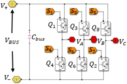
In this exposition, Insulated Gate Bipolar Transistors (IGBTs) are used as the controlling semiconductors in the converter circuit [17], as seen in Figure 3. The most commonly used PWM control strategies are SPWM control strategy, THIPWM control strategy, and SVPWM control strategy.
Figure 3. Three-phase H-Bridge converter
3.1 Sinusoidal PWM control strategy
The Sinusoidal PWM (SPWM or Triangle Comparison TCPWM) employs three-phase sinusoids as the reference signals ($V_a^*, V_b^*, V_c^*$) that are 120 degrees out of phase with each other and compares them with the triangle carrier waves to produce the signals for the switch gates. In comparison to the modulating signal, the carrier signal has a high frequency. In addition, to obtain a high-quality output voltage and to prevent high switching losses in semiconductors, this frequency shouldn't be set too high. These two parameters are known as frequency and amplitude modulation indices, denoted by (mf and ma) respectively. The modulation indices (ma and mf) signal amplitude and frequency are used to control the fundamental output voltage of the converter. The ratio of the peak value of the reference signal $V_m^*$ to the peak value of the carrier signal Vtri. is known as the amplitude modulation index ma. On the other hand, the ratio of the carrier frequency ftri to the reference signal frequency f* is known as the frequency modulation index mf.
$m_a=\frac{V_m^*}{V_{t r i.}}, m_{\mathrm{f}}=\frac{\mathrm{f}_{t r i .}}{\mathrm{f}^*}$ (16)
The fundamental component's magnitude and frequency can be adjusted using the ratio modulation indices (ma and mf), which are key design factors. The amplitude modulation ratio ma is adjusted by changing the amplitude of the modulating signals while keeping the triangle comparison signals constant [18]. Frequency modulation indices mf are changed by varying the triangle signal frequency while keeping the frequency-modulating signal constant. The frequency modulation index is always greater than one [19].
For normal steady-state operation, 0<ma≤1 is referred to as linear modulation. In transient, when the peak of the sinusoidal reference signal is greater than the peak of the carrier wave (i.e., ma>1), the inverter cannot provide a fundamental voltage proportional to the voltage reference. When the frequency of the sinusoidal reference wave is higher than the frequency of the triangle waves, the system is overmodulated. The conventional bipolar PWM (two-level topologies) is done between zero and Vdc voltage levels. In a three-phase H-bridge converter, two switches on the same leg will operate in complementary mode, meaning that when one is turned ON, the other is turned OFF, and vice versa. Referred to Figure 3, the output voltages are controlled as follows: $S_1$ is "1" when $V_a^*>V_{t r i.}$, $\mathrm{~S}_4$ is "1" when $V_a^*<V_{t r i.}$, $\mathrm{~S}_3$ is "1" when $V_b^*>V_{t r i .}$, $\mathrm{S}_6$ is "1" when $V_b^*<V_{t r i .}$, $\mathrm{S}_5$ is "1" when $V_c^*>V_{t r i.}$, and $\mathrm{S}_2$ is "1" when $V_c^*<V_{t r i.}$.
Figure 4. Simulink model of (2L- VSI) based on PWM
Figure 5. Operating principle of output voltage simulations SPWM
The Simulink implementation of the RSC (2L-VSI) model is shown in Figure 4, while Figure 5 shows the output voltage of the simulation for Va, Vb and Vc.
3.2 Sinusoidal PWM technique with third harmonic injection (THIPWM)
It might be able to achieve an output voltage that is higher in amplitude than when utilizing sine PWM [20]. Typically, a sinusoidal reference signal is enhanced by the addition of a third harmonic signal [21]. This is known as Third Harmonic Injection Modulation (THIPWM).
As shown in Figure 6, the reference signal, on the other hand, has two maxima equal to one at $\theta_1=\frac{\pi}{3}$ and $\theta_2=\frac{2 \pi}{3}$, at $\omega t=\frac{\pi}{3}$.
Voltage taken $\frac{V_{bus }}{2}$, the equations can now be written as follows:
$\frac{V_{bus }}{2}=V_{1( max. )} \sin \left(\frac{\pi}{3}\right), \Rightarrow V_{1( max. )}=0.577 V_{bus }$ (17)
The equations for the fundamental component V1 and triple-frequency V3 are as follows:
$\left[\begin{array}{l}V_1=1.1547 \sin \theta \\ V_3=0.193 \sin 3 \theta\end{array}\right]$ (18)
For each phase, the output voltage waveform with third harmonic components is represented as the study [22].
$\left[\begin{array}{c}1.1547 v_m^*\left[\sin (\theta)+\frac{1}{6} \sin (3 \theta)\right] \\ 1.1547 v_m^*\left[\sin \left(\theta-\frac{2 \pi}{3}\right)+\frac{1}{6} \sin \left(3 \theta-\frac{2 \pi}{3}\right)\right] \\ 1.1547 v_m^*\left[\sin \left(\theta+\frac{2 \pi}{3}\right)+\frac{1}{6} \sin \left(3 \theta+\frac{2 \pi}{3}\right)\right]\end{array}\right]$ (19)
Figure 6. The third harmonic is injected to enhance the amplitude fundamental component
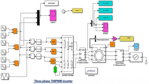
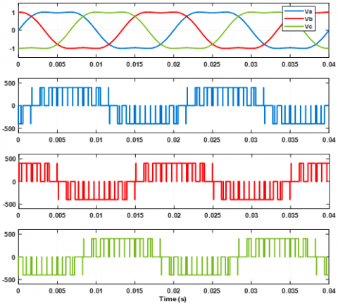
The Simulink model of a two-level VSI based on THIPWM, with its operating principle and corresponding inverter regions [23], is shown in Figure 7. The aim of the THIPWM technique, as shown in Figure 8, are to increase the maximum utilization of the DC link with a reduction in the THD of the output voltage, and this approach improves the RSC's performance. In addition, it is possible to modify the amplitude modulation index in linear range modulations as follows: (1<ma≤1.15) [24].
Figure 7. Simulink model of two-level VSI based on THIPWM
Figure 8. Operating principle of output voltage simulations THIPWM
3.3 Space vector modulation (SVPWM) control strategy
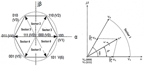
The SVPWM differs from other SPWM methods in that it uses a reference vector. It has the benefit of giving a better process for the system. The concept of space vectors is to describe the three-coordinate plane, including the three phases’ vectors in a two-coordinate plane by utilizing the (abc/αβ) Clarke transformation. Thus, one of the most used PWM techniques is called (SVPWM). The position of the reference V* on αβ- coordinate plane controls whether the switches that are ON or OFF. To achieve the minimum switching frequency of each inverter leg, the switching state sequence must be configured in such a way that the change from one state to the next is achieved by switching just one bit. The switching state of the top switch (S1, S3, S5) and bottom switch (S2, S4, S6) complimentary in each leg [25]. Table 1 demonstrates that there are two possible states ON, which means “1”, and OFF, which means “0” for the switches [26]. Accordingly, there are (23=8) possible combinations of switching states that could occur so that, two (000, 111) are zero switching states placed in the axis of origin and six (001, 010, 011, 100, 110, and 110) are active switching states, as shown in Figure 9.
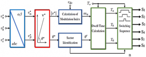
A block diagram in Figure 10 provides a step-by-step description of how to design SVPWM for a (2L-VSC).
Table 1. The sequence switching state for each sextant
|
Angle θ |
Switches State |
Sector |
|
0° ≤ θ ˂ 60° |
000 100 110 111 110 100 000 |
1st (Start right) |
|
60° ≤ θ ˂ 120° |
000 010 110 111 110 010 000 |
2nd (Start left) |
|
120° ≤ θ ˂ 180° |
000 010 011 111 011 010 000 |
3rd (Start right) |
|
180° ≤ θ ˂ 240° |
000 001 011 111 011 001 000 |
4th (Start left) |
|
240° ≤ θ ˂ 300° |
000 001 101 111 101 001 000 |
5th (Start right) |
|
300° ≤ θ ˂ 360° |
000 100 101 111 101 100 000 |
6th (Start left) |
Generally, for each sector number (n), the dwell times equations can be generalized as follows [27]:
$T_a=\frac{\sqrt{3}\left|V^*\right| T_S}{V_{d c}} \sin \left(\frac{\pi}{3} n-\theta\right)$ (20)
$T_b=\frac{\sqrt{3}\left|V^*\right| T_S}{V_{d c}} \sin \left(\theta-(n-1) \frac{\pi}{3}\right)$ (21)
$T_0=T_s-T_a-T_b$ (22)
where, n=1, 2, 3, 4, 5, and 6; Ts=Sampling time (switching time).
The reference voltage in three-phase balanced systems is as follows [28]:
$\left\{\begin{array}{c}v_a^*=v_m \sin (\omega \mathrm{t}) \\ v_b^*=v_m \sin \left(\omega t-\frac{2 \pi}{3}\right) \\ v_c^*=v_m \sin \left(\omega t+\frac{2 \pi}{3}\right)\end{array}\right.$ (23)
The Clark transformer, also known as the (αβ) transformer, converts a three-dimensional (a b c) coordinate (e.g., current, voltage, flux) into a stationary two-phase system (αβ). If zero-sequence is eliminated from the transformation matrices, the Clarke transformation matrix representation is given by Eq. (24).
$\left[\begin{array}{l}v_\alpha \\ v_\beta\end{array}\right]=\frac{2}{3}\left[\begin{array}{ccc}1 & -\frac{1}{2} & -\frac{1}{2} \\ 0 & \frac{\sqrt{3}}{2} & -\frac{\sqrt{3}}{2}\end{array}\right]\left[\begin{array}{l}v_a \\ v_b \\ v_c\end{array}\right]$ (24)
In the αβ-frame, the reference voltage vector V* is as follows:
$V^*=v_\alpha+j v_\beta$ (25)
This vector's magnitude and angle can be calculated as follows:
$\left|V^*\right|=\sqrt{\left(v_\alpha\right)^2+\left(v_\beta\right)^2}$ (26)
$\theta=\tan ^{-1}\left(\frac{v_\beta}{v_\alpha}\right)$ (27)
The length of the reference vector denotes as |V*| and the angle denotes as θ*. The reference vector is used to precise the control of the magnitude and frequency of the output voltage waveform [29]. A length of the reference voltage and the value of the DC-bus voltage are used to determine the modulation index ma:
$m_a=\frac{\sqrt{3}\left|V^*\right|}{V_{d c}}$ (28)
Figure 9. Configuration of space vector converters (2L-VSC)
Figure 10. The block diagram of three-phase two-level SVPWM
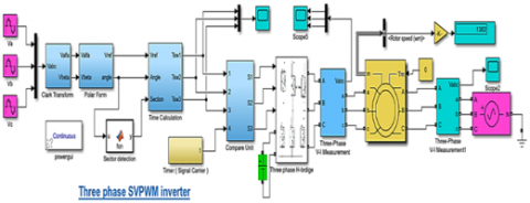
The Simulink model of (2L-VSI) that is based on SVPWM is shown in Figure 11, while the operating principle is seen in Figure 12 [30].
Figure 11. Simulink model of (RSC) two-level VSI based on SVPWM
Figure 12. Operating principle of output voltage simulations SVPWM
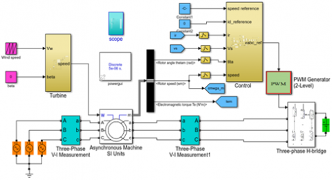
Figure 13. Simulation control circuit of DFIG-RSC
In recent years, many research papers have reviewed different algorithms and techniques that contribute to tracking the maximum PowerPoint to the WECs for different variable speeds. The algorithms are categorized according to direct electrical power Pele control (DPC) measurement, indirect mechanical power Pwind control (IPC), and hybrid to capture the extracted maximum power MPPT from WECS. It can be classified into four main control strategies: Tip Speed Ratio (TSR) control, Perturb and Observe (P&O) or Hill-Climb Searching (HCS) control, Power Signal Feedback (PSF), and Optimum Torque Control (OTC). The control strategy has been implemented to control the active and reactive power flows. The modeling and simulation are built using MATLAB/Simulink software for the DFIG wind turbine using the different PWM techniques depicted in Figure 13.
The control strategy has been implemented using the DPC method to control the active and reactive power flows. the rotor voltage equations in the (d/q) frame [9]. The assumption is that power losses in stator and rotor resistances are neglected, and the $\frac{d \Psi_S}{d t}$ stator flux vector may be taken as roughly equaling zero because the stator winding links to the AC electrical network (infinite bus). The d-axis is aligned (reference frame) with the stator flux vector in this analysis (Note that: Ψds=Ψs and Ψqs=0), substituting in Eq. (5), obtains:
$\left\{\begin{array}{c}v_{d s}=0 \\ v_{q s}=\Psi_s \omega_s=v_s\end{array}\right.$ (29)
The power (active/reactive) equation can be found through Eqs (11) and (12), and Eq. (29):
$\left\{\begin{array}{l}P_s=\frac{3}{2}\left(\Psi_s \omega_s i_{q s}\right) \\ Q_s=\frac{3}{2}\left(\Psi_s \omega_s i_{d s}\right)\end{array}\right.$ (30)
From Eqs. (7) and (8), the stator current, can be written as follows [31]:
$\Psi_s=L_s i_{d s}+L_m i_{d r}$ (31)
$0=L_s i_{q s}+L_m i_{q r}$ (32)
The stator current can be written as follows:
$\left\{\begin{array}{c}i_{d s}=\frac{L_m i_{d r}-\Psi_s}{L_s} \\ i_{q s}=\frac{L_m i_{q r}}{L_s}\end{array}\right.$ (33)
Substituting Eq. (33) into Eq. (30), which yields:
$\left\{\begin{array}{c}P_S=-\frac{3}{2}\left(\frac{L_m \Psi_s \omega_s}{L_s} i_{q r}\right) \\ Q_s=-\frac{3}{2}\left(\frac{L_m \Psi_s \omega_s}{L_S} i_{d r}-\frac{\Psi_S^2 \omega_s}{L_S}\right)\end{array}\right.$ (34)
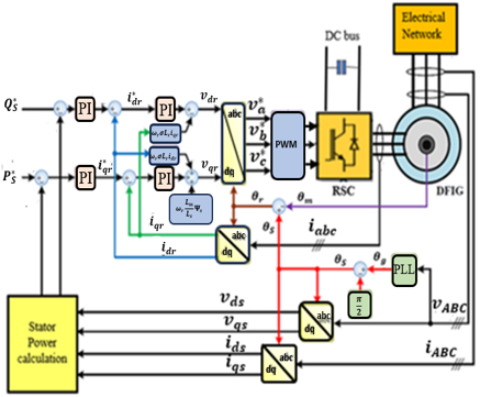
The above equations show that the quadrature rotor and the direct rotor current components are proportional to the stator's active and reactive stator's power, as shown in Figure 14. Therefore, the rotor voltages are derived by multiplying Eqs. (8) and (9) by the Lm and Ls, respectively, to obtain:
$L_m \Psi_{q s}=L_m L_s i_{q s}+L_m^2 i_{q r}$ (35)
$L_s \Psi_{q r}=L_s L_r i_{q r}+L_m L_s i_{q s}$ (36)
Then, Eq. (36) is subtracted from Eq. (35), and the result equation is divided by Ls, yielding:
$\Psi_{q r}=\frac{L_m}{L_s} \Psi_{q s}+\sigma L_r i_{q r}=\sigma L_r i_{q r}$ (37)
where, $\sigma=\left(1-\frac{L_m^2}{L_r L_S}\right)$.
Similarly
$\Psi_{d r}=\frac{L_m}{L_S} \Psi_s+\sigma L_r i_{d r}$ (38)
The rotor voltage is obtained by substituting Eqs. (37) and (38) into rotor voltage Eq. (6), it will be shown that the rotor voltage is proportional to stator flux and rotor current.
$v_{d r}=R_r i_{d r}+\sigma L_r \frac{d}{d t} i_{d r}-\omega_r \sigma L_r i_{q r}+\frac{L_m}{L_s} \frac{d \Psi_s}{d t}$ (39)
$v_{q r}=R_r i_{q r}+\sigma L_r \frac{d}{d t} i_{q r}+\omega_r \sigma L_r i_{d r}+\omega_r \frac{L_m}{L_s} \Psi_s$ (40)
The tracking errors active $\left(e_{P_s}=P_s^*-P_s\right)$ and reactive $\left(e_{Q_s}=Q_s^*-Q_s\right)$ stator powers' between the set-point and actual values [32].
Figure 14. Block schematic of the DFIG-RSC power control system
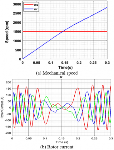
Indeed, DFIG can work in the hyper or hypo-synchronous mode. Figure 15 (a) depicts the mechanical speed, and Figure 15 (b) illustrates the rotor current during a transition from the sub-synchronous to the super-synchronous mode [33]. A back-to-back power electronic is utilized on the RSC-PWM converter to control the direction of the power flow between the rotor-DFIG and the network.
Figure 15. Rotor side control of DFIG
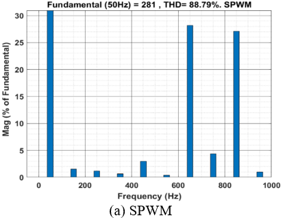
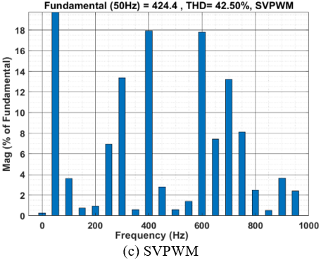
The modelling and simulation of (7.5 KW-DFIG) coupled with a wind turbine used in Simulink of MATLAB are the output frequency of the grid (f=50Hz), DC voltage (Vdc=400V), ma=0.8, and mf=15. All the results of Simulink models and FFT can be seen. It can be shown that the harmonic component THD values of the output voltage of SPWM, THIPWM, and SVPWM techniques are 85.79%, 50.35%, and 42.50% respectively, as investigated in Figures 16 (a), 16 (b) and 16 (c). The THD factor was found in the SVPWM to be lower than the other techniques. Because THD values indicate the quality and reliability of the control system and power quality. On the other hand, the SVPWM modulation technique is challenging to implement particularly in the over-modulation region. The harmonic current, overmodulation strategy complexity, and smooth transfer between the linear and overmodulation regions are important problems with the overmodulation strategy. These problems can affect power converters' performance, stability, and efficiency.
Figure 16. Total harmonic distortion (THD) result applied to DFIG-RSC
The essential purpose of any PWM strategy is to generate variable output with a high fundamental component, minimal harmonics, and easy implementation. This paper begins modeling DFIG and evaluates the difference between SPWM, THIPWM, and SVPWM techniques. A suitable PWM strategy to drive a back-to-back converter is used to improve stability and dynamic performance. According to the paper's results, the fundamental voltage component can be raised by 15.5% more SPWM using the SVPWM approach in the under-modulation region for the same DC bus voltage. The increase in the amplitude of the fundamental voltage on applying PWM strategies is significant because the system can deliver more power to the network. On the other side, SVPWM has made it easier to implement digital control VSCs and better utilize control techniques. The future directions of PWM method development two-level to multilevel PWM-B2B converters, such as the hybrid multilevel, are to improve the system's flexibility and programmability, minimize the THD of the output voltage and current, and reduce the hardware's complexity.
|
DFIG |
Doubly fed induction generator |
|
B2B |
Back-to-back |
|
PMSG |
Permanent magnet synchronous generators |
|
SPWM |
Sinusoidal pulse width modulation |
|
THD |
Total harmonic distortion |
|
THIPWM |
Third-harmonic injection PWM |
|
SVPWM |
Space vector pulse width modulation |
|
GSC |
Grid side converter |
|
RSC |
Rotor side converter |
|
FFT |
Fast fourier transform |
|
Lm |
Mutual inductance, H |
|
Ls, Lr |
Stator and rotor self-inductances, H |
|
Rs, Rr |
Stator and rotor resistances, Ω |
|
Ψds, Ψqs |
Stator flux vector in d,q-axis, Wb |
|
Ψdr, Ψqr |
Rotor flux vector in d,q-axis, Wb |
|
ids, iqs, idr, iqr |
Stator and rotor current in d,q-axis, A |
|
vds, vqs |
Stator voltage in d,q components, V |
|
vdr,vqr |
Rotor voltage in d,q components, V |
|
Ps, Qs |
Active and reactive powers of stator, Kw |
|
Pr, Qr |
Active and reactive powers of rotor, Kw |
|
$e_{P_S}, e_{Q_S}$ |
Errors active and reactive stator power |
|
Ωm |
Rotational speed of the wind turbine, (rad/sec) |
|
Tem |
Electromagnetic torque, N⋅m |
|
Tm |
Mechanical torque, N⋅m |
|
J |
Moment of inertia, Kg.m2 |
|
f |
Total friction factor constant (DFIG and turbine), Nm.s |
|
Pp |
No. of pole pairs |
|
R |
Blade radius, m2 |
|
vw |
Wind speed, m/s |
|
Cp |
Power co-efficient |
|
ωs |
Synchronous angular speed, rad/sec |
|
ωr |
Angular speed of rotor, rad/sec |
|
Greek symbols |
|
|
ρair |
1.225 kg/m3 air density in kg/m3, (e.g., and a temperature of 15℃ at sea level) |
|
b |
Blade pitch angle |
|
λ |
Tip speed ratio |
|
σ |
Leakage coeffiecient |
The characteristics of DFIG used in simulation parameters are noted in Table A1.
Table A1. The parameters of DFIG
|
Parameter |
Value |
Unit |
|
DFIG-rated power Pg |
7.5 |
KW |
|
Stator rated voltage |
400 |
V |
|
Moment of inertia J |
0.15 |
Kg.m2 |
|
Friction factor constant |
0.05 |
N.m.s |
|
No. of pair of poles |
2 |
- |
|
Frequency |
50 |
Hz |
|
Rs |
0.5968 |
Ω |
|
Rr |
0.6258 |
Ω |
|
Lis |
0.00547 |
H |
|
Lir |
0.00547 |
H |
|
Lm |
0.0354 |
H |
[1] Asuhaimi, A., Pesaran, M., Khairuddin, A., Jahanshaloo, L., Shariati, O. (2013). An overview on doubly fed induction generators′ controls and contributions to wind-based electricity generation. Renewable and Sustainable Energy Reviews, 27: 692-708. https://doi.org/10.1016/j.rser.2013.07.010
[2] Desalegn, B., Gebeyehu, D., Tamirat, B. (2022). Wind energy conversion technologies and engineering approaches to enhancing wind power generation: A review. Heliyon, 8(11): E11263. https://doi.org/10.1016/j.heliyon.2022.e11263
[3] Jha, D. (2017). A comprehensive review on wind energy systems for electric power generation: Current situation and improved technologies to realize future development. International Journal of Renewable Energy Research, 7(4): 1786-1805. https://doi.org/10.20508/ijrer.v7i4.6264.g7219
[4] Xu, D., Blaabjerg, F., Chen, W., Zhu, N. (2018). Advanced Control of Doubly Fed Induction Generator for Wind Power Systems. John Wiley & Sons.
[5] Suleyman, N., Sahin, Y. (2018). Effects to system performance of different PWM techniques in field oriented speed control with back-to-back converter of PMSG. Academic Platform-Journal of Engineering and Science, 6(2): 34-44. https://doi.org/10.21541/apjes.321310
[6] Bektache, A., Boukhezzar, B. (2018). Nonlinear predictive control of a DFIG-based wind turbine for power capture optimization. International Journal of Electrical Power & Energy Systems, 101: 92-102. https://doi.org/10.1016/j.ijepes.2018.03.012
[7] Luo, X. (2021). Design of an adaptive controller for double-fed induction wind turbine power. In 2021 International Conference on Energy Engineering and Power Systems, Hangzhou, China, pp. 1622-1626. https://doi.org/10.1016/j.egyr.2021.09.047.
[8] Benbouhenni, H., Boudjema, Z., Belaidi, A. (2020). Power control of DFIG in WECS using DPC and NDPC-NPWM methods. Mathematical Modelling of Engineering Problems, 7(2): 223-236. https://doi.org/10.18280/mmep.070208
[9] Ahmad, H., Khalid, H., Amin, A., Masroor, N., Mahmood, H., Abubakar, M. (2021). Improved current controlled doubly fed induction generator model with grid integration under sub and super synchronous conditions. Journal of Electrical Engineering & Technology, 16(1): 141-153. https://doi.org/10.1007/s42835-020-00572-w
[10] Navas, M.A.H., Puma, J.L.A., Filho, A.J.S. (2015). Direct torque control for squirrel cage induction generator based on wind energy conversion system with battery energy storage system. In 2015 IEEE Workshop on Power Electronics and Power Quality Applications (PEPQA), Bogota, Colombia, pp. 1-6. https://doi.org/10.1109/PEPQA.2015.7168203
[11] Benbouhenni, H., Mehedi, F., Soufiane, L. (2022). New direct power synergetic-SMC technique based PWM for DFIG integrated to a variable speed dual-rotor wind power. Automatika: Časopis za Automatiku, Mjerenje, Elektroniku, RRačunarstvo i Komunikacije, 63(4): 718-731. https://doi.org/10.1080/00051144.2022.2065801
[12] Wang, J., Bo, B. (2022). Adaptive fixed-time sensorless maximum power point tracking control scheme for DFIG wind energy conversion system. International Journal of Electrical Power & Energy Systems, 135: 1-9. https://doi.org/10.1016/j.ijepes.2021.107424
[13] Zadehbagheri, M., Sutikno, T., Kiani, M. (2023). A new method of virtual direct torque control of doubly fed induction generator for grid connection. International Journal of Electrical and Computer Engineering, 13(1): 1201-1214. https://doi.org/10.11591/ijece.v13i1.pp1201-1214
[14] Sitharthan, R., Karthikeyan, M., Sundar, D., Rajasekaran, S. (2020). Adaptive hybrid intelligent MPPT controller to approximate effectual wind speed and optimal rotor speed of variable speed wind turbine. ISA Trans, 96: 479-489. https://doi.org/10.1016/j.isatra.2019.05.029
[15] Aykut, O., Ulu, C., Komurgoz, G. (2022). Modeling, control, and experimental verification of a 500 kW DFIG wind turbine. Advances in Electrical and Computer Engineering, 22(1): 13-20. https://doi.org/10.4316/AECE.2022.01002
[16] Ting, N., Yasa, Y., Aksoy, I., Sahin, Y. (2015). Comparison of SVPWM, SPWM and HCC control techniques in power control of PMSG used in wind turbine systems. Aegean Conference on Electrical Machines & Power Electronics, pp. 69-74. https://doi.org/10.1109/OPTIM.2015.7426976
[17] Boopathi, R., Jayanthi, R., Ansari, M. (2020). Maximum power point tracking-based hybrid pulse width modulation for harmonic reduction in wind energy conversion systems. Computers & Electrical Engineering, 86: 106711. https://doi.org/10.1016/j.compeleceng.2020.106711
[18] Kumar, M., Shenoy, K., Praveen, G. (2020). PWM techniques to power converters of the wind energy conversion system. In IEEE 9th International Conference on Communication Systems and Network Technologies (CSNT), Gwalior, India, pp. 155-160. https://doi.org/10.1109/CSNT48778.2020.9115754
[19] Bhattacharjee, T., Jamil, M., Jana, A. (2018). Design of SPWM based three phase inverter model. In Technologies for Smart-City Energy Security and Power (ICSESP), Bhubaneswar, India, pp. 1-6. https://doi.org/10.1109/ICSESP.2018.8376696
[20] Jose, J., Goyal, G., Aware, M. (2010). Improved inverter utilisation using third harmonic injection. In 2010 Joint International Conference on Power Electronics, Drives and Energy Systems & Power India, New Delhi, India, pp. 1–6. https://doi.org/10.1109/PEDES.2010.5712490
[21] Tan, B., Gu, Z., Shen, K., Ding, X. (2018). Third harmonic injection SPWM method based on alternating carrier polarity to suppress the common mode voltage. IEEE Access, 7: 9805-9816. https://doi.org/10.1109/ACCESS.2018.2890014
[22] Belkheiri, A., Aoughellanet, S., Belkheiri, M., Rabhi, A. (2015). FPGA based control of a PWM inverter by the third harmonic injection technique for maximizing DC bus utilization. In 2015 3rd International Conference on Control, Engineering & Information Technology (CEIT), Tlemcen, Algeria, pp. 1-7. https://doi.org/10.1109/CEIT.2015.7233028
[23] Moura, L., Reis, A., Lima, M., Oliveira, J., Santos, I. (2019). Experimental evaluation of wind turbines inverters on generating harmonic currents. International Journal of Emerging Electric Power Systems: 20(1): 1-16. https://doi.org/10.1515/ijeeps-2018-0210
[24] Thakre, M., Gangurde, J., Shriwastava, R., Kadam, D., Kadlag, S., Sonawane, H. (2022). Investigative uses of overmodulation techniques in modular multilevel cascaded converter. Bulletin of Electrical Engineering and Informatics, 11(6): 3147-3156. https://doi.org/10.11591/eei.v11i6.3958
[25] Xu, J., Soeiro, T., Gao, F., Chen, L., Tang, H., Bauer, P., Dragičević, T. (2021). Carrier-based modulated model predictive control strategy for three-phase two-level VSIs. IEEE Transactions on Energy Conversion, 36(3): 1673–1687. https://doi.org/10.1109/TEC.2021.3073110
[26] Tarusan, S., Jidin, A., Jamil, M., Karim, K., Sutikno, T. (2020). A review of direct torque control development in various multilevel inverter applications. International Journal of Power Electronics and Drive Systems, 11(3): 1675-1688. https://doi.org/10.11591/ijpeds.v11.i3.pp1675-1688
[27] Al-Anbary, K., Kadhum, H., Al-hayder, A. (2021). Modeling, simulation and analysis of doubly-fed induction generator for wind turbines under grid voltage fluctuation. Journal of University of Babylon for Engineering Sciences, 29(3): 27-49.
[28] Bhukya, R., Kumar, P. (2020). Simplified down sampling factor based modified SVPWM technique for cascaded inverter fed induction motor drive. International Journal of Advances in Applied Sciences, 9(1): 20-26. https://doi.org/10.11591/ijaas.v9.i1.pp20-26
[29] Sevilmiş, F., Karaca, H. (2014). Simulation and analysis of SVPWM based VSI for wind energy systems. In Proceedings of the 2014 6th International Conference on Electronics, Computers and Artificial Intelligence (ECAI), Bucharest, Romania, pp. 73-78. https://doi.org/10.1109/ECAI.2014.7090151
[30] Mayoral, E., Reyes, E., Cortez, R., Mercado, E., García, V., Gosebruch, R. (2021). Modeling and validation of the switching techniques applied to back-to-back power converter connected to a DFIG-based wind turbine for harmonic analysis. Electronics, 10(23): 1-29. https://doi.org/10.3390/electronics10233046
[31] Elbashir O.E., Zezhong W., Qihui L. (2014). Modeling and analysis of DFIG in wind energy conversion system. International Journal of Energy Environment, 5(2): 239-250.
[32] Alhato, M. Mazen, Bouallègue, S., Rezk, H. (2020). Modeling and performance improvement of direct power control of doubly-fed induction generator-based wind turbine through second-order sliding mode control approach. Mathematics, 8(11): 2012-2020. https://doi.org/10.3390/math8112012
[33] Pena, R., Clare, J., Asher, G. (1996). Doubly fed induction generator using back-to-back PWM converters and its application to variable-speed wind-energy generation. IEE Proceedings-Electric Power Applications, 143(3): 231-241. https://doi.org/10.1049/ip-epa:19960288