Nahida Naji Kadhim![]() | Layla H. Abood
| Layla H. Abood![]() | Yousra Abd Mohammed*
| Yousra Abd Mohammed*![]()
© 2023 IIETA. This article is published by IIETA and is licensed under the CC BY 4.0 license (http://creativecommons.org/licenses/by/4.0/).
OPEN ACCESS
In recent years, electric vehicles have garnered significant attention due to their environmental and economic advantages compared to conventional vehicles, including reduced emissions and lower fuel costs. This study proposes an optimal fractional-order PID (FOPID) controller to regulate electric vehicle (EV) speed. The FOPID controller is advantageous due to its ability for stabilizing the system, managing parameter variations, and mitigating potential disturbances. The tuning of this controller's gains is achieved through an intelligent Ant Colony Optimization (ACO) algorithm. The selection of the gain values is strategically based on minimizing error, thereby ensuring a robust system response without overshoot or undershoots. The performance of the proposed controller is analyzed and compared to a classical PID controller for demonstrating its superior performance. Simulation results illustrate the efficiency of the proposed controller, which exhibits no fluctuation or oscillation in its response (zero overshoot) and fast settling and rise times of 0.0476 and 0.0297, respectively. By using the optimal gains determined by the smart ACO, the proposed controller achieves a satisfactory and robust system response in controlling EV speed.
electric vehicle, fractional-order PID (FOPID), speed control, sunflower optimization
The motor is regarded as the significant part of an EV framework, beside to the regulator, drive train, charger and power supply. Regulator is the core of an EV, and the key for the acknowledgment of an elite presentation EV with an ideal equilibrium of most extreme speed lately, in view of worldwide fuel supply, contamination issues and an Earth-wide temperature boost; zero-dirtying types of electric vehicles are a quickly developing innovation for power the board and ecological saving issue [1]. Electrical vehicles have been presented in the industry marketing [2]. Moreover, the DC motors can give best job and regarded as a braking tool due to their facilities in its fast torque behavior [3].
Various studies are utilized in the survey for adjusting its power, the price and raising driving levels in order to enhance the power maintaining issue [4, 5]. A linear quadratic controller that controls the position of the throttle was presented in the study [6] for hybrid electric vehicles. However, the closed-loop system’s performance reduces when a linear type of controller is used with the nonlinear plants. A fuzzy logic controller is adopted for controlling a permanent magnet synchronous motor’s speed was developed and experimentally tested in the study [7]. A robust cruise control system for a DC motor in EV was proposed in the study [8]. To compensate for the effects of changes in vehicle weight and the road grade, numerical optimization is used with the suggested. In the study [9], the EV has two inputs. The linear velocity and the steering angle. The linear velocity is enhanced by a Permanent magnet motor type and the steering angle is presented with a stepper motor type. In cruise control, a steady speed was achieved. In the study [10], a neural network-based PI is proposed for an EV driven by induction motor drives. In fact, power electronics and motor drives are actively researching neural network concepts, and in the study [11], an adaptive neural network approach is used to control an EV based on an interior permanent magnet synchronous machine (IPMSM), the adaptive scheme was presented depending on the Lyapunov relation for achieve stability to ensure robustness, and best tracking. In the study [12] for optimizing the control of an electric vehicle system, new technique was created depending on stochastic drive cycles. A sliding mode controller for EV was presented in the study [13]. In the study [14], a feedback linearization method was used to the Light Weight EV (LWEV) system. In this method, the linear system was adjusted by using LQR controller.
In this study, an augmented and enhanced controller is adopted, its depend on fractional calculus by adding two parameters in fraction form to the integral and differentiator gains, its named as a FOPID controller which is adopted for controlling speed of EV based on using a unique and intelligent ACO algorithm for finding the gains controller to improve the EV system dynamic behavior and obtain a stable and robust behavior. This study is organized as: Section 2 explains the EV system modeling. Section 3 indicates the adopted controller used. Section 4 indicated the ACO algorithm, Section 5 demonstrates the simulation results then and then in Section 6, a conclusion is presented.
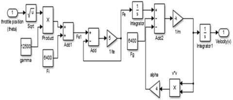
This section of the paper is presented an electronic speed control schematic graph which employing a DC servo motor appears in Figure 1, the vehicle’s dynamics are modeled using the leader-follower configurations [6]. The electric vehicle (EV) depicted in Figure 1 that utilizes an electronic throttle control method is also known as a single-mode power split, either in series or parallel, or both. A planetary gear system starts the power supply to the wheels in both series and parallel configurations. While the series flow technique gets electricity from the engine to the battery and then back from the electrical system to the wheels, the parallel flow method uses two paths: one from the engine to the wheels and another from the battery, to the motors, and back to the wheels. This construction improves overall performance, reduces pollution, and has high speed levels, among other advantages. The throttle plate is rotated by a DC servo motor in this electronic throttle control system, and its rotation is managed by the voltage provided to the motor [15].
Figure 1. The electronic throttle control diagram
Eqs. (1)-(3) can be used to calculate the relationship between follower vehicle’s acceleration, propulsion force, and drag forces: [6, 16] where Fe (Engine force, a throttle position function), Fg (Gravitational Force, A road grade function: is 30% of weight of vehicle), θ (throttle position), v (EV speed), and τe (Engine time constant commonly lie between 0.1 to 1sec., here is taken 0.2s). The variables adopted for work is presented in Table 1.
$m \frac{d v}{d t}=F_e(\theta)-\alpha v^2-F_g$ (1)
$\tau_e \frac{d F_e(\theta)}{d t}=-F_e(\theta)+F_{e 1}(\theta)$ (2)
$F_{e 1}(\theta)=F_1+\gamma \sqrt{\theta}$ (3)
Table 1. Numerical parameters values
|
Constant |
Notation |
Value (SI unit) |
|
Vehicle mass |
$m$ |
1000Kg |
|
Aerodynamic drag coefficient |
$\alpha$ |
4N/(m/s)2 |
|
Engine force coefficient |
$\gamma$ |
12500N |
|
Engine idle force |
$F_1$ |
6400N |
Eq. (1) through (3) are used to build the Simulink model of the vehicle seen in Figure 2 [17]. Eq. (4) through (7) display the state variable representation of the vehicle, and Eq. (8) displays the transfer function.
$A=\left[\begin{array}{lll}0 & 0.001 ; & 0\end{array}-5\right]$ (4)
$B=\left[0 ; 8.29 \times 10^8\right]$ (5)
$C=\left[\begin{array}{ll}1 & 0\end{array}\right]$ (6)
$D=[0]$ (7)
$\frac{V(s)}{\theta(s)}=\frac{8.29 \times 10^5}{s(s+5)}$ (8)
The Eigenvalues of the open-loop system are λ1=0 and λ2=−5, which are derived from the characteristic equations of the system expressed in Eqs. (4)–(7).
Ẋ(t)=Ax(t)+Bu(t) is the equation for a linear time invariant (LTI) system. The system matrix A is represented by n×n, the control matrix B by n×r, and the input vector matrix u by r×1 dimensions. A controlled and observable system exists when the rank of matrix M = [B AB A2B ... An−1B] is n. Given that matrix M and N's order equals the matrix's rank of 1 [18]; $\mathrm{M}=829000\left[\begin{array}{cc}0 & 0.001 \\ 0 & -5\end{array}\right]$, $\mathrm{N}=\left[\begin{array}{ll}1 & 0 \\ 0 & 1\end{array}\right]$.
Figure 2. EV simulink model
PID controllers is regarded as a simple and classical controllers that adopted for improving system behavior. Nowadays, studies are made with a different changes for PID controller like combining it with a neural network [19, 20] or changing its structure to reach to a best stability and robustness as in [21, 22] or changing it by add a fractional variables (integral & derivative) to the classical PID to improve system output [23, 24], this type of change is an augmented type PID controller. These parameters (μ for derivative variable and λ for the integral variable) make the gains of controller be five variables. In the automation and control fields, the Fractional Order Controllers (FOCS) achieve more accurate and stable performances, it is classified into four types: CRONE controller, Tilt and Integral (TID) controller type, FOPID controller and fractional-order lead-lag compensator, it is consists of five variables: three normal gains and named proportional, integral, and derivative while there is a two fractional variables for integral and derivative, representing the FOPID can be expressed using a graph of PID controller that explained by the plane of the μ and λ variables that appeared in Figure 3 [25].
Figure 3. Fractional PID controller plane
In 1695, L'Hopital used the phrase fractional order calculus to illustrate how some systems may be properly described using fractional order differential equations. On this, Lurel, Riemann, Laplace, Able, and Euler act. Calculus in fractional order is studied more quickly starting in 1884. Differential is a key variable in fractional order calculus. Since the two fractional order type’s derivative and integrator may be expressed by a single operator, this name has become popular. The following is an explanation of the differintegral [26, 27]:
$\mathrm{aD}_{\mathrm{t}}^\alpha=\left\{\begin{array}{c}\frac{d^\alpha}{d t^r} R(\alpha)>0 \\ 1 R(\alpha)=0 \\ \int_\alpha^t(d \tau)^{-a} R(\alpha)<0\end{array}\right.$ (9)
The operator's boundaries in Eq. (9) are "a" and "t.", "α" represents the operation's order and is linked to R, (any rational number) it might even be a complex number. Specifically, the Riemann-Louville (RL) expression and the Grunwald-Letnikov (GL) expression are chosen to represent the basic fractional differintegral. The definition of GL is
$\mathrm{aD}_{\mathrm{t}}^\alpha \mathrm{f}(\mathrm{t})=\lim _{h \rightarrow 0} h^{-\alpha} \sum_{j=0}^{\frac{t-\alpha}{h}}(-1)^j\left(\begin{array}{l}\alpha \\ j\end{array}\right) \mathrm{f}(\mathrm{t}-\mathrm{jh})$ (10)
The fractional differintegral represented by RL is:
$\mathrm{aD}_{\mathrm{t}}^{\mathrm{r}} \mathrm{f}(\mathrm{t})=\frac{1}{\Gamma(n-\alpha)} \frac{d^n}{d t^n} \int_\alpha^t \frac{f(\tau)}{\left.(t-\tau)^{(a}-n+1\right)} d \tau$ (11)
For (n-1<α<n) and Γ (.) is the Gamma function.
In this study, a FOPID controller is adopted [28, 29] to controlling the speed in EV system its structure is indicated in Figure 4 and its transfer function is indicated in Eq.(12) below:
$G_{\mathrm{FOPID}}=K_{\mathrm{P}}+K_{\mathrm{I}} \frac{1}{s^\lambda}+s^\mu K_{\mathrm{D}}$ (12)
Figure 4. FOPID structure
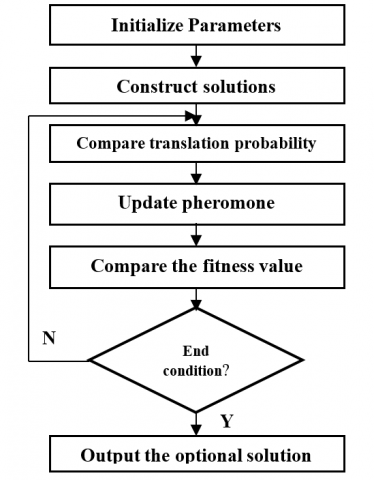
Figure 5. ACO flow chart
ACO is a population-based strategy that translates the combinatorial method of optimization; it emulates the mechanism by which actual ants locate the shortest path when conducting searches inside their colony. Each ant will secrete a chemical material called pheromone; it will dispose this material behind it and each ant will follow other ants depending on the concentration of pheromone which indicate the short way among other far routes of their way. In ACO, a finite number of artificial ants are initiated. Each one will take a decision to solve the problem. During this, each ant gives its decision based on the problem utilized and on its own behavior. The best decision is adopted based on its fitness function then their decisions are represented by the path selected. ACO must find an optimal way either locally or globally. The path details found during their trip is saved in the pheromone attempts relayed to their different paths. Pheromone attempts will be the memory for all ants’ trips. They are decided their final decision and change their ways depending on the pheromone trials and update it to the optimal path [30, 31], the flow chart of ant colony is indicated in Figure 5 and the steps of ACO algorithm are given as follows:
Step 1: Initialize the ACO parameters like dimension of the problem $(\operatorname{dim})$, population size $(N)$, maximum number of iterations (Iter), alpha $(\alpha)$, beta $(\beta)$, Evaporation rate $(\rho)$, pheromone Matrix $(\tau)$, and change of pheromone $(\Delta \tau)$.
Step 2: Find the probability for each ant in solving the way according to Eq. (13).
$P_{i j}^k(t)=\frac{\left[\tau_{i l}(\mathrm{t})\right]^\alpha\left[\eta_{i l}\right]^\beta}{\sum_{l \in N_i^k}\left[\tau_{i l}(\mathrm{t})\right]^\alpha\left[\eta_{i l}\right]^\beta}$ (13)
Step 3: Calculate the minimum Integral Time Absolute Error (ITAE) cost function [32, 33] indicated in Eq. (14) below at each tour depending on the best ode minimum value. At each tour a test is done to find the best ant that find the optimal decision.
$\mathrm{n} I T A E=\int_0^{\infty} t|\mathrm{e}| d t$ (14)
Step 4: Each ant will have a pheromone hormone on her way and it is calculated as indicated in Eq. (15) below:
$\tau_{i l}(t+1)=\tau_{i l}(t)+\sum_{k=1}^m \Delta \tau_{i l}^k(t) \forall(i, j) \in L$ (15)
where, $\Delta \tau_{i l}^k(t)$ is the pheromone value in the way of the kth ant in the iteration tour and the amount of pheromone value will be calculated using Eq. (16).
$\Delta \tau_{i l}^k(t)=\left\{\begin{array}{c}1 / L_K \quad \forall(i, j) \in L \\ 0 \text { otherwise }\end{array}\right.$ (16)
where, L is the road length during tour iteration. Based on step 3 the updated process will do just to the ant that find the optimal path in which it should be allowed to lead elite.
Step 5: Now when the evaporation is completed then the pheromones updated according to Eq. (17) as shown:
$\tau_{i l}(+t 1)=(\mathbf{1}-\rho) \tau_{i l}(t)+\Delta \tau_{i l}^k(t)$ (17)
where, 0< $\rho$ <1 is the 'evaporation factor' .
All of the ants update their data and determine whether or not the maximum iteration was achieved after calculating the pheromone and finishing the evaporation.
Step 6: Check the maximum iterations (Iter) value, if it is reached it will stop, otherwise, Step 2 to Step 5 is repeated. The FOPID controller is adopted to enhance the dynamical behavior by reduce error between desired and actual values by continuously compute the (ITAE) fitness function suggested, the issue is how to select the optimal values the FOPID variables based on ACO by choosing these values in each iteration then check the fitness function when it is minimized to a suitable value the process will stop in the suitable iteration to measure the tuned values of FOPID controller gains.
Figure 6. EV system with proposed controller based on ACO algorithm
Figure 6 explain the proposed controller used for controlling EV speed based on ACO algorithm.
This section explains the simulation results for the recommended optimal controller for EV speed control using Matlab software version 2019. To improve system response, the ACO algorithm is adopted; its initial parameters are chosen based on the literature, and its iteration number and population are chosen through trials to produce quick and accurate results. The results are shown in Table 2 below.
Table 2. ACO parameters
|
Description |
Value |
|
ANT population |
100 |
|
Number of iteration |
30 |
|
Pheromone variable |
1 |
|
Evaporation variable |
0.05 |
|
Initial concentration |
1.5 |
|
Heuristic variable |
2 |
|
Pheromone |
100 |
|
Initial uniform probability |
0.5 |
|
Controller gains |
5 |
In this study the, the ITAE fitness function equation is used for monitoring the error during simulation and based on its value the ACO algorithm will find a controller gains. system response is shown in Figure 7.
FOPID's ability to provide the desired reaction quickly and steadily is confirmed by a comparison with two traditional controllers (optimal PID and classical PID). Figure 8 show its superiority upon the two controllers used, Table 3 list the gains of all controller tested and Table 4 explain the transit analysis for each controller.
Table 4 makes it clear that the recommended FOPID controller outperforms the two conventional controllers that were employed (PID, Optimal PID) in its transient analysis and try to reach its desired speed with best settling time (0. 0476) while in classical PID and optimal PID are slow and equal to 0.235s and 0.093s respectively, also its faster in its rise time with value equal to 0.0297s with respect to classical PID and Optimal PID with a value equal to 0.163 and 0.062s respectively. This deviation in classical PID is due to its simple structure with a manually chosen gain values and its effect reflected on system response while the optimal PID give a response better than the classical PID but still not reach to the FOPID controller stable response, then by analyzing system response a stable behavior is shown clearly without any overshoot and fluctuations in its response this is due to the fractional parameters effect and the efficient tuning algorithm used in selecting the more suitable and tunable controller gains that achieve its best performance.
Figure 7. Response EV speed
Figure 8. System response for all controllers
Table 3. All controllers gains
|
Controller |
Kp |
KI |
KD |
λ |
μ |
|
Classical PID |
0.01 |
0.044 |
0.0016 |
- |
- |
|
Optimal PID |
0.008552 |
0.0633 |
0.0005 |
- |
- |
|
FOPID |
0.00041 |
0.000067 |
0.00091 |
0.891 |
0.985 |
Table 4. Comparative results of response parameters
|
Controller |
Max. Overshoot (Mp%) |
Peak Time (tp) |
Rise Time (tr) |
Settling Time (ts) |
|
Classical PID |
0.25 |
0.45 |
0.163 |
0.235 |
|
Optimal PID |
0.2 |
0.19 |
0.062 |
0.093 |
|
FOPID |
0 |
0.08 |
0.0297 |
0.0476 |
In this study a FOPID controller is adopted for maintaining speed in EV system, a smart optimization method is used for finding the suitable values for controller gains and improves system behavior by minimizing error level between desired speed and actual speed also by tracking the suitable desired speed with a stable output and without any fluctuating values. A comparison analysis with the other controllers indicates that the proposed controller is more efficient in achieving best analysis values; it is faster than classical PID by 79.44% and optimal PID by 48.81% in rise time and faster than classical PID by 81.77% and optimal PID by 52.09% in settling time with a stable response level, this controller can be implemented in different embedded systems due to its efficient structure and all gains is calculated offline which reduce any delay may happen. The suggested controller with its fractional variables and the best optimizing algorithm maintain a best and efficient desired response with an optimal level values. In future work, many ideas can be suggested like make a hybrid system with intelligent methods like neural or fuzzy systems to enhance system performance.
For help in finishing this study, the authors are grateful to the University of Technology in Baghdad-Iraq.
[1] Wang, R.R., Jing, H., Yan, F.J., Karimi, H.R., Chen, N. (2015). Optimization and finite-frequency H∞ control of active suspensions in in-wheel motor driven electric ground vehicles. Journal of the Franklin Institute, 352(2): 468-484. https://doi.org/10.1016/j.jfranklin.2014.05.005
[2] De Santiago, J., Bernhoff, H., Ekergård, B., Eriksson, S., Ferhatovic, S., Waters, R., Leijon, M. (2011). Electrical motor drivelines in commercial all-electric vehicles: A review. In IEEE Transactions on Vehicular Technology, 61(2): 475-484. https://doi.org/10.1109/TVT.2011.2177873
[3] Sharma, V., Purwar, S. (2014). Nonlinear controllers for a light-weighted all-electric vehicle using chebyshev neural network. International Journal of Vehicular Technology, 2014: 1-15. https://doi.org/10.1155/2014/867209
[4] Lin, F.J., Hung, Y.C., Hwang, J.C., Chang, I.P., Tsai, M.T. (2012). Digital signal processor-based probabilistic fuzzy neural network control of in-wheel motor drive for light electric vehicle. IET Electric Power Applications, 6(2): 47-61. https://doi.org/10.1049/iet-epa.2011.0153
[5] Yu, K., Tan, X., Yang, H., Liu, W., Cui, L., Liang, Q. (2016). Model predictive control of hybrid electric vehicles for improved fuel economy. Asian Journal of Control, 18(6): 2122-2135. https://doi.org/10.1002/asjc.1304
[6] Yadav, A.K., Gaur, P., Jha, S.K., Gupta, J.R.P., Mittal, A.P. (2011). Optimal speed control of hybrid electric vehicles. Journal of Power Electronics, 11(4): 393-400. https://doi.org/10.6113/jpe.2011.11.4.393
[7] Choi, H.H., Jung, J.W. (2011). Takagi-sugeno fuzzy speed controller design for a permanent magnet synchronous motor. Mechatronics, 21(8): 1317-1328. https://doi.org/10.1016/j.mechatronics.2011.07.012
[8] Diba, F., Arora, A., Esmailzadeh, E. (2014). Optimized robust cruise control system for an electric vehicle. Systems Science & Control Engineering: An Open Access Journal, 2(1): 175-182. https://doi.org/10.1080/21642583.2014.891956
[9] Vighneswaran, G., Nair, K.S. (2018). Speed control of electric vehicle with sliding mode controller. International Research Journal of Engineering and Technology (IRJET), 5(5): 388-391.
[10] Gasbaoui, B., Nasri, A., Abdelkhalek, O. (2016). An efficiency PI speed controller for future electric vehicle in several topology. Procedia Technology, 22: 501-508. https://doi.org/10.1016/j.protcy.2016.01.109
[11] Chaoui, H., Khayamy, M., Okoye, O. (2018). Adaptive RBF network based direct voltage control for interior PMSM based vehicles. IEEE Transactions on Vehicular Technology, 67(7): 5740-5749. https://doi.org/10.1109/TVT.2018.2813666
[12] Schwarzer, V., Ghorbani, R. (2012). Drive cycle generation for design optimization of electric vehicles. IEEE Transactions on Vehicular Technology, 62(1): 89-97. https://doi.org/10.1109/TVT.2012.2219889
[13] Nasri, A., Hazzab, A., Bousserhane, I.K., Hadjeri, S., Sicard, P. (2010). Fuzzy logic speed control stability improvement of lightweight electric vehicle drive. Journal of Electrical Engineering & Technology, 5(1): 129-139. https://doi.org/10.5370/jeet.2010.5.1.129
[14] Huang, Q., Huang, Z., Zhou, H. (2009). Nonlinear optimal and robust speed control for a light-weighted all-electric vehicle. IET Control Theory & Applications, 3(4): 437-444. https://doi.org/10.1049/iet-cta.2007.0367
[15] Yadav, A.K., Gaur, P. (2014). Robust adaptive speed control of uncertain hybrid electric vehicle using electronic throttle control with varying road grade. Nonlinear Dynamics, 76(1): 305-321. https://doi.org/10.1007/s11071-013-1128-9
[16] Kaur, J., Saxena, P., Gaur, P. (2013). Genetic algorithm based speed control of hybrid electric vehicle. In 2013 Sixth International Conference on Contemporary Computing (IC3), IEEE, 65-69. https://doi.org/10.1109/IC3.2013.6612163
[17] Bisht, P., Yadav, J. (2020). Optimal speed control of hybrid electric vehicle using GWO based fuzzy-PID controller. In 2020 International Conference on Advances in Computing, Communication & Materials (ICACCM), IEEE, 115-120. https://doi.org/10.1109/ICACCM50413.2020.9212985
[18] Singh, A., Kaur, E.A. (2014). Speed control of hybrid electric vehicle using optimization algorithm. International Journal of Advanced Research in Computer and Communication Engineering, 3: 6856-6860.
[19] Hattim, L., Karam, E.H., Issa, A.H. (2018). Implementation of self tune single neuron PID controller for depth of anesthesia by FPGA. In New Trends in Information and Communications Technology Applications, Springer International Publishing, 159-170. https://doi.org/10.1007/978-3-030-01653-1_10
[20] Abood, L.H., Karam, E.H., Issa, A.H. (2018). FPGA implementation of single neuron PID controller for depth of anesthesia based on PSO. In 2018 Third Scientific Conference of Electrical Engineering (SCEE), IEEE, 247-252. https://doi.org/10.1109/SCEE.2018.8684186
[21] Abood, L.H. (2022). Optimal modified PID controller for automatic voltage regulation system. In AIP Conference Proceedings, AIP Publishing, 2415: 030007. https://doi.org/10.1063/5.0092583
[22] Abood, L.H., Kadhim, N.N., Abd Mohammed, Y. (2023). Dual stage cascade controller for temperature control in greenhouse. Bulletin of Electrical Engineering and Informatics, 12(1): 51-58. https://doi.org/10.11591/eei.v12i1.4328
[23] Abood, L.H., Ali, I.I., Oleiwi, B.K. (2022). Design a robust fractional order TID controller for congestion avoidance in TCP/AQM system. In 2022 26th International Computer Science and Engineering Conference (ICSEC), IEEE, 366-370. https://doi.org/10.1109/ICSEC56337.2022.10049311
[24] Abood, L.H., Haitham, R. (2022). Design an optimal fractional order PI controller for congestion avoidance in internet routers. Mathematical Modelling of Engineering Problems, 9(5): 1321-1326. https://doi.org/10.18280/mmep.090521
[25] Wan, J.H., Liu, W.Q., Ding, X., He, B., Nian, R., Shen, Y., Yan, T.H. (2018). Fractional order PID motion control based on seeker optimization algorithm for AUV. In OCEANS 2018 MTS/IEEE Charleston, IEEE, 1-4. https://doi.org/10.1109/OCEANS.2018.8604500
[26] Tan, N., Yüce, A., Deniz, N.F. (2016). Teaching fractional order control systems using interactive tools. The Eurasia Proceedings of Educational & Social Sciences.
[27] Aydoğdu, Ö., Korkmaz, M. (2019). Optimal design of a variable coefficient fractional order PID controller by using heuristic optimization algorithms. International Journal of Advanced Computer Science and Applications, 10(3). https://doi.org/10.14569/ijacsa.2019.0100341
[28] Ibrahim, E.K., Issa, A.H., Gitaffa, S.A. (2022). Optimization and performance analysis of fractional order PID controller for DC motor speed control. Journal Européen des Systémes Automatisés, 55(6): 741-748. https://doi.org/10.18280/jesa.550605
[29] Abood, L.H., Oleiwi, B.K. (2021). Design of fractional order PID controller for AVR system using whale optimization algorithm. Indonesian Journal of Electrical Engineering and Computer Science, 23(3): 1410-1418. https://doi.org/10.11591/ijeecs.v23.i3.pp1410-1418
[30] Kumar, R., Singh, R., Ashfaq, H. (2020). Stability enhancement of multi-machine power systems using ant colony optimization-based static synchronous compensator. Computers & Electrical Engineering, 83: 106589. https://doi.org/10.1016/j.compeleceng.2020.106589
[31] Sandoval, D., Soto, I., Adasme, P. (2015). Control of direct current motor using ant colony optimization. In 2015 CHILEAN Conference on Electrical, Electronics Engineering, Information and Communication Technologies (CHILECON), IEEE, 79-82. https://doi.org/10.1109/Chilecon.2015.7400356
[32] Abd Mohammed, Y., Abood, L.H., Kadhim, N.N. (2023). Design and simulation an optimal enhanced PI controller for congestion avoidance in TCP/AQM system. TELKOMNIKA (Telecommunication Computing Electronics and Control), 21(5): 997-1004. https://doi.org/10.12928/telkomnika.v21i5.24872
[33] Abood, L.H., Oleiwi, B.K., Humaidi, A.J., Al-Qassar, A.A., Al-Obaidi, A.S.M. (2023). Design a robust controller for congestion avoidance in TCP/AQM system. Advances in Engineering Software, 176: 103395. https://doi.org/10.1016/j.advengsoft.2022.103395