Nadia Lachtar*![]() | Imen Driss
| Imen Driss![]()
© 2023 IIETA. This article is published by IIETA and is licensed under the CC BY 4.0 license (http://creativecommons.org/licenses/by/4.0/).
OPEN ACCESS
Scheduling problems in the industrial sector are among the most studied optimization problems. Improving resource efficiency and minimizing production costs have become important concerns for industry managers. Seeking the best way to maximize profit is now a primary objective for any business. This is the context in which our study is positioned. It focuses on the resolution of job shop scheduling problems (JSSP). Considering that production challenges in industries are complex and require the consideration of multiple factors, we turn to the use of artificial intelligence tools for their resolution. Pharmaceutical manufacturing often involves a large number of resources, machines, and tasks, leading to high complexity in the JSSP. Ant colony optimization (ACO) is innovative and excels in its ability to handle this complexity by seeking optimal solutions while avoiding computational pitfalls. It can efficiently explore vast search spaces and leverage ant parallelism to reach the best solution in a short period of time, which is crucial in the pharmaceutical context where deadlines and quality constraints are paramount. Thus, in order to address the JSSP, this work suggests and puts into practice a method that involves the application of an ACO approach with the goal of minimizing the makespan. We validated our approach by comparing it with various algorithms through benchmarks taken from the published research. The suggested approach proved to be effective as the produced solutions were of high quality and showed that it could achieve results that are closer to the ideal solution for larger-scale issues than other algorithms with an average percentage relative error of just 0.67%. Furthermore, application of ACO in the context of BIOCARE's pharmaceutical laboratories’ production led to an improvement of approximately 3 hours in their weekly planning.
BIOCARE, ant colony optimization, genetic algorithm, industry, job shop scheduling problem, OR-TOOLS, particle swarm optimization, taboo search
The JSSP is complex and multifaceted conundrum that has garnered the attention of researchers and industrialists alike. The JSSP represents an issue in operations management, where a multitude of jobs with varying processing requirements must be allocated to a limited set of machines while adhering to specific constraints, ultimately seeking to minimize makespan, which is the total completion time. The JSSP transcends industrial domains, making its study and resolution essential across various sectors as manufacturing, healthcare, transportation, and logistics. It presents a multitude of real-world scenarios where the allocation of limited resources, such as machines, personnel, or vehicles, to a set of tasks with distinct processing sequences. The consequences of efficient JSSP are far-reaching, with the potential to reduce operational costs, enhance productivity, improve delivery times, and maintain high levels of customer satisfaction.
The primary aim of JSSP is to determine an ideal plan that reduces the makespan, representing the overall time needed to finish all tasks, to a minimum. The JSSP is widely recognized as NP-hard, indicating that obtaining an exact optimal solution within a reasonable time is computationally infeasible for large problem instances. As such, scholars have turned to heuristic and metaheuristic techniques to address this complex scheduling problem. One such powerful metaheuristic approach is ACO that draws inspiration from ant foraging behavior. It employs pheromone trails left by simulated ants to facilitate optimization processes and discover valid solutions in a graph. During the optimization process, multiple ants explore the search space represented as a directed graph, and upon reaching a terminal vertex, the solution is derived from the path they found. As the process unfolds, these simulated ants leave pheromones behind, which serve as a guide for other ants to either replicate the same solution or explore neighboring areas. ACO has demonstrated significant success in solving combinatorial optimization problems. It has been effectively used to solve a variety of scheduling issues and is especially appropriate for issues with discrete solution areas. This paper is structured in the following manner: Section 2 provides an overview of the primary contributions relevant to our research. In Section 3, we delve into the presentation of the mathematical and graphical modeling of the problem. Section 4 outlines the suggested approach for addressing JSSP. Section 5 presents the experiments, results, and discussions, where we examine the outcomes of the experiments conducted to assess the effectiveness of the ACO solution we have put forth. It addresses the various algorithms drawn from the literature and compares them to our adapted ACO algorithm, including constraint programming, genetic algorithm (GA), tabu search (TS), and particle swarm optimization (PSO). The algorithms are tested on benchmark instances of different sizes to evaluate their performance and effectiveness. Section 6 details the application of our algorithm to a real-life case within the pharmaceutical products laboratory (at BIOCARE). A conclusion and future works are described in section 7.
Finally, it is worth noting that many algorithms are commonly used to solve small-scale JSSP and provide optimal solutions. However, it is clearly evident that there is a gap in solving large-scale JSSP. This gap presents a significant opportunity for future research in this field. Therefore, this article focuses on the adaptation and implementation of ACO to resolve large-scale JSSP, aiming to provide insights into its effectiveness and potential as a scheduling optimization tool, In addition to its usage to a real case in the pharmaceutical industry. This research aims to provide a unique perspective to the field by addressing this specific aspect of the pharmaceutical industry.
The JSSP has garnered significant attention in the realms of operations research and industrial engineering because of its practical significance and intricate nature. Several approaches have been proposed for addressing the JSSP, among them, exact methods such as the widely used branch-and-bound approach [1-3]. Another exact method employed for combinatorial problems is Answer Set Programming (ASP) [4, 5]. ASP has demonstrated successful applications in real-world scenarios, spanning across industries [6] to fields like biology and medicine [7]. A recurring challenge with these precise methods is their efficiency in managing instances of modest scale, whereas they encounter difficulties when confronted with larger instances. To address large-scale metaheuristics, are used like TS [8-11]. In addition, Artificial intelligence techniques play a crucial role in resolving job shop scheduling problems [12-14]. Among these techniques, the GA stands out as one of the most prevalent [15-17], along with other population-based approaches like PSO [18, 19] and ACO algorithms [20-22] whether operating on evolutionary or swarm principles, offer significant flexibility and generate solutions for scheduling issues that, while not achieving absolute precision, exhibit satisfactory accuracy within a reasonable time frame. Furthermore, population algorithms can be combined in hybrid configurations with deterministic methodologies [15-17, 23].
To contextualize our choice of ACO in our study, we provide a brief comparison of job shop problem-solving methods mentioned in the literature in terms of their strengths and weaknesses:
The studies conducted by the studies [20-22] primarily focused on small to medium-sized instances of the JSSP. In contrast, our work aims to explore the efficiency of ACO on large-scale problems.
In the following, we will provide the notations for the data used within the scope of our problem: $\boldsymbol{\Omega}$: Set of all available machines, $\boldsymbol{n}$: Total number of jobs, $\boldsymbol{m}$: Total number of machines, $\boldsymbol{i}$: Index of the $\boldsymbol{i}^{\boldsymbol{t h}}$ job, $\boldsymbol{j}$: Index of the $\boldsymbol{j}^{\boldsymbol{t h}}$ operation of job $\boldsymbol{i}, \boldsymbol{J}_{\boldsymbol{i o}}$: Total number of operations in job $\boldsymbol{J}_{\boldsymbol{i}}, \boldsymbol{O}_{\boldsymbol{i} \boldsymbol{j}}$: $\boldsymbol{j} \boldsymbol{t} \boldsymbol{h}$ Operation of job $\boldsymbol{J}_{\boldsymbol{i}}, \boldsymbol{\Omega}_{i j}$: Set of available machines for operation $\boldsymbol{O}_{i j}, \boldsymbol{p}_{i j}{ }^{\boldsymbol{k}}$: Execution time of operation $\boldsymbol{O}_{i j}$ on machine k and $\boldsymbol{S}_{i j} \boldsymbol{k}^{\boldsymbol{k}}$: Start time of operation $\boldsymbol{O}_{i j}$ on machine k.
3.2 Mathematical modeling
The model we provide is based on the formulation according to the study [24].
Objective function:
$\operatorname{Minimize}\left[\operatorname{Max}\left(C_{1 j 1}, C_{2 j 2}, \ldots C_{n j n}\right)\right]$ (1)
Subject to:
$C_{i j}-S_{i j}-P_{i j}=0 \forall i=1 . . n, j=1 . . m$ (2)
$\begin{gathered}C_{i^{\prime} j^{\prime}}-C_{i j}+H\left(1-Y_{i j i^{\prime} j^{\prime}}\right) \geq \\ P_{i^{\prime} j^{\prime}} \forall(i, j), \forall\left(i^{\prime}, j^{\prime}\right): O_{i j} \in N_k, O_{i^{\prime} j^{\prime}} \in N_k\end{gathered}$ (3)
$\begin{gathered}C_{i j}-C_{i^{\prime} j^{\prime}}+H\left(Y_{i j i^{\prime} j^{\prime}}\right) \geq \\ P_{i j} \forall(i, j), \forall\left(i^{\prime}, j^{\prime}\right): O_{i j} \in N_k, O_{i^{\prime} j^{\prime}} \in N_k\end{gathered}$ (4)
$S_{i j} \geq 0 \forall i, j$ (5)
$S_{i j+1}-C_{i j} \geq 0 \forall i, j=1, \ldots, J_{i-1}$ (6)
$Y_{i j i^{\prime} j^{\prime}}=\left\{\begin{array}{c}1, \text { if operation } o_{i j} \text { precedes } o_{i\prime j \prime} \\ 0, \text { otherwise }\end{array}\right.$ (7)
In this context, we have $S_{i j}$ and $C_{i j}$ denoting the initiation and finalization times for job $\mathrm{i}$, where $\mathrm{H}$ is a significantly large positive integer. Additionally, $\mathrm{N}_{\mathrm{k}}$ represents the group of operations $\left\{\mathrm{O}_{\mathrm{ij}}\right\}$ that can be allocated to machine $\mathrm{k}$, and $\mathrm{Y}_{\mathrm{iji^{\prime}j^{\prime}}}$ is a decision variable establishing a sequence between operations $\mathrm{O}_{\mathrm{ij}}$ and $\mathrm{O}_{\mathrm{ij} \mathrm{i^{\prime}j}^{\prime}}$.
Constraint 2: Intra-job precedence constraint: An operation within the same job cannot commence until the previous operation within that job has been completed.
Constraints 3, 4: Resource sharing constraint: Each machine is limited to handling a single operation at any given moment.
Constraint 5: This constraint states that the initiation time for each operation must be greater than or equal to zero.
Constraint 6: This constraint ensures that the value of the makespan must be greater than or equal to the completion times of the last operations for all jobs.
3.2 Graphical modeling
The JSSP is commonly portrayed using a disjunctive graph $\mathrm{G}=(\mathrm{V}, \mathrm{C} \cup \mathrm{D})$ to represent tasks and resources, with $\mathrm{V}$ representing the nodes corresponding to operations, excluding the initial node (I) and terminal nodes (F) in the graph. C represents a set of directed edges $(\rightarrow)$ connecting operations within the same job (technological sequence), and D denotes a set of undirected edges $(\leftarrow---\rightarrow)$ linking operations executed on the same machine. Furthermore, the processing time of each operation is indicated at the upper part of the node.
4.1 Elitist ACO
To optimize the Makespan, we propose the utilization of an elitist ACO algorithm, where the problem is modeled as a disjunctive graph and the transition between vertices is carried out using Eq. (8)
$P_{i j}=\frac{\left(\tau_{i j}\right)^\alpha\left(\eta_{i j}\right)^\beta}{\sum_L\left(\tau_{i L}\right)^\alpha\left(\eta_{i L}\right)^\beta}$ (8)
where, $P_{i j}$ represents the transition probability from vertex i to vertex $\mathrm{j}, \tau_{i j}$ denotes the pheromone amount for the arc i to $\mathrm{j}, \alpha$ defines the impact of pheromone, $\eta_{i j}$ indicates the desirability of $i, j$ edge, $\beta$ defines the impact of the desirability. $\sum_L\left(\tau_{i L}\right)^\alpha\left(\eta_{i L}\right)^\beta$ is the summation of the product of pheromones and distances over all available transitions from vertex $\mathrm{i}$.
The desirability of an edge is determined by a weighting function, primarily based on heuristics, which assigns a value indicating the quality or attractiveness of that edge. The weighting function $\eta_{i j}$ can be defined as follows:
$\eta_{i j}=\frac{1}{d_{i j}}$ (9)
where, $\mathrm{d}_{\mathrm{ij}}$ is the length of the edge $\mathrm{i}, \mathrm{j}, \mathrm{d}_{\mathrm{ij}}=\boldsymbol{p}_{i j} \boldsymbol{k}$, it represents the processing time of operation $\mathrm{j}$ of job $\mathrm{i}$ by machine $\mathrm{k}$ in the case of JSSP.
$\alpha$ and $\beta$ are vital factors guiding the decision-making process of each ant $(\mathrm{k})$ by shaping their edge selection, taking into account pheromone levels $(\tau)$ and the heuristic data $(\eta)$ correspondingly. The objective is to ensure that edges with higher pheromone levels are more visible, resulting in a higher transition probability to other nodes within the group of attainable operations. To seek the parameters $\alpha$ and $\beta$, different methods are considered, such as reviewing the literature and comparing with reference data, consulting experts, conducting empirical testing, using parameter tuning techniques, and employing automatic parameter adaptation. In our paper, we use literature review and benchmarking methods. So, from the literature, we find that the usual way to specify the parameters $\alpha$ and $\beta$ is as numerical values, and the following relationship is established: $\beta=1-\alpha$, with $\alpha \in[0,1]$.
The equation 10 defines the quantity of pheromone $\tau_{i j}$ found on each edge of the pathway in the generation $t$.
$\tau_{i j}=\sum_{k=1}^n \Delta \tau_{i j}{ }^k+\rho * \tau_{i j}(t-1)$ (10)
The term $\tau_{i j}{ }^k$ symbolizes the ant's part in the current generation $t$ overall pheromone. The amount of evaporation is represented by $\rho$. To make sure that previous pheromone levels do not considerably affect the ants' future judgments, the amount of evaporation must be included. Eq. (11) defines the inverse relationship between the value of the solution and the pheromone production provided by every ant, which is based on the standard of the response it finds.
$\Delta \tau_{i j}{ }^k=\frac{Q}{L_k}$ (11)
In this context, Q represents a fixed value. $\mathrm{L}_{\mathrm{k}}$ denotes the makespan duration corresponding to the result that $\mathrm{k}$ ant has discovered. In order to accelerate the approach's convergence, all elitist ants' (e) knowledge is used to improve the pheromone trail's transparency on the best path's vertices. Therefore, Eq. (12) is used instead of Eq. (11) to determine the optimal route established for each period.
$\Delta \tau_{i j}{ }^k=\frac{Q}{L_k}(\mathrm{e})$ (12)
4.2 JSSP elitist ACO
The approach's fast convergence may lead to a reduction in exploration capacity, as the ants quickly converge to one path, that has the potential to produce a local optimum. In order to counterbalance the issue, the algorithm allows the inclusion of operations in the set of feasible choices that may delay or pause machine execution for a certain amount of time if that specific task remains running on another device. But these actions can only be chosen if there is enough pheromone present on the edge that connects to the node, making the probability of selection higher than operations with immediately available jobs. This preference for delaying operations requires a large amount of pheromone, with the attribute of unused devices are undesirable and penalize the process by making it less visible.
The approach seeks to produce a wide range of solution by thoroughly exploring the search space, generating a diverse set of solutions, some of which may surpass the local optima initially discovered during the early iterations. These superior solutions act as limits, guiding the search and preventing it from stopping too close to the global optimum, ensuring that the algorithm continues searching for solutions that are distant from the global optimum by up to 5%. The initial diversity of the algorithm is crucial in directing the ants towards the exploration of the solution space, where the path leading to the total best solution can be identified. The pseudocode used to solve the JSSP is as follows:
Algorithm
(1) Initialization of parameters: $\alpha, \beta, \rho, e$ Ants and $\mathrm{C}$ cycles
(2) For each edge $a_{i j}$ do:
$\tau_{0 i j}=c$ where $\mathrm{c}$ is a constant
$\Delta \tau_{i j}=0$ actual pheromone accumulator
(3) For every cycle $\mathrm{C}$ do:
3.1. Random assignment of the first operation
3.2. Define the decidability rule for each ant $k$
3.3. While $t a b u_k$ is not full do:
For every ant $k$ do:
Determine the set of operation achievable from the current node Select the next operation to be visited according to Eq. (8)
Move the ant to the selected operation Save the selected operation in $t a b u_k$
3.4. For every ant $k$ do:
Determine the makespan $L_k$ makspan of the constructed plan
Store the plan with the lowest makespan
from cycle C
For every edge $a_{i j}$ do:
Calculate $\Delta \tau_{i j}$ according to equation 11 or 12
3.5. For every edge $a_{i j}$ do:
Update pheromone $\tau_{i j}$ according to equation 10
$\Delta \tau_{i j}=0$
3.6. Display the shortest plan from cycle C
3.7. $t a b u_k=\phi$ Clear the list of visited elements
(4) Display the plan with the shortest makespan Gantt diagram is built and displayed.
Algorithm description
According to the literature, the parameter values are defined as follows: $\alpha=0.2, \beta=0.8$, and $\rho=0.7$, Cycles $C=1000$, and the jobs $\mathrm{n}$ determines ants e, which is computed as $e=\frac{n}{2}$.
Pheromone values are initialized to small positive values. The stochastic building stage of solutions starts with e ants. Within the limitations of the task, a random selection is made from the nodes that are first visited for the initial operation. By equivalent chance, the decision strategy that takes the least computation time or the greatest execution time of the operations is chosen at random. Ants continue to traverse the graph until the $\mathrm{tabu}_{\mathrm{k}}$ memory is fully populated. There are $\mathrm{n} \times \mathrm{m}+2$ operations in total. To avoid revisiting, the $\mathrm{tabu}_{\mathrm{k}}$ list limits the options for operations. Operations with delays of five-time units or fewer are included. After every ant builds a solution, pheromones are revised according to equation 10 . Pheromones are released at visited edges. Following each algorithmic cycle, this global update is carried out, and the pheromone accumulator is then reset. Finally, the algorithm presents the shortest makespan and generates the Gantt diagram.
Implementation of elitist ACO for JSSP
We implemented the system as a Windows application. For this, we used IntelliJ IDEA (version 2023.1.1, released on April 28, 2023). It is an integrated development environment (IDE) for Java technology used in software development. It is developed by JetBrains, available as open source under the Apache 2 license, and supports the Java programming language. We also utilized the following tools: JDK 9 (Java Development Kit).
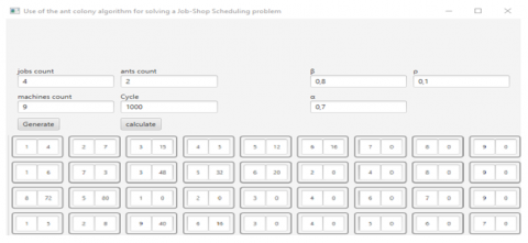
Below are the steps and the screenshot of the program's execution using the FT06 job shop instance data.
First, we input n (jobs), m (machines) and the parameters. Afterward, clicking "Generate" creates a matrix with rows representing jobs and columns representing machines. Each row i fits with job i containing m operations. Each operation j is modeled by a cell containing two fields. The first field corresponds to machine k that processes operation j. The duration of the execution of operation j of task i by machine k is denoted by the second field (see Figure 1). The matrix is being filled according to the data.
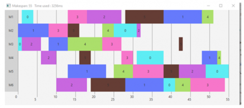
Finally, we click the "Calculate" button, which displays the makespan and generates the Gantt diagram (see Figure 2).
Figure 1. The data for the job shop instance FT06
Figure 2. Makespan and Gantt diagram of FT06
To validate our approach, we utilized the following benchmark instances: FT: Fisher and Thompson [25], LA: Lawrence [26], Applegate and Cook [27], YN: Li et al. [28], TA: Taillard [29] and ABZ: Adams et al. [30]. We used the following database.
Table 1 displays, the authors’ names, the instance name, its dimension and the optimal solution taken from the studies [25-28, 30].
We also utilized the following algorithms:
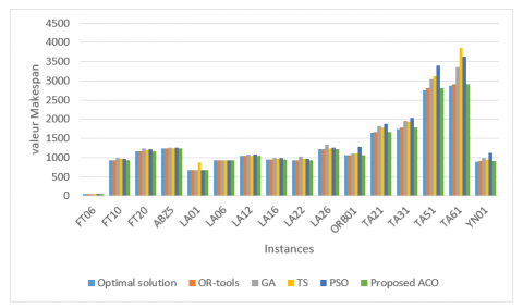
Table 2 compares the outcomes of the suggested ACO compared to various other approaches (OR-Tools, GA, TS, PSO) running on the selected databases. Each cell indicates the best makespan and the execution time in seconds in parenthesis. It shows also the percentage relative error by instances sizes and approaches and the percentage relative error average by approach. The last row of Table 2 displays the t-test results and the corresponding p-values obtained using the t-test statistic to compare the optimal solution with the solutions produced by the algorithms
By setting a significance threshold (confidence level) at 0.05, it becomes evident that all calculated p-values for the algorithms are higher than this threshold. This observation implies that we lack sufficient evidence to assert that the differences between the optimal solutions and the solutions generated by the algorithms are statistically significant. Therefore, it suggests that the algorithms are statistically equivalent to the optimal solution, producing results comparable to the optimal outcome. Consequently, one can conclude that the algorithms are effective in the resolution of the JSSP.
Table 1. Database
|
Authors |
Instances |
Sizes |
Optimal Solution |
|
Fisher and Thompson |
FT06 |
6×6 |
55 |
|
FT10 |
10×10 |
930 |
|
|
FT20 |
20×5 |
1165 |
|
|
Adams, Balas and Zawack |
ABZ5 |
10×10 |
1234 |
|
Lawrence |
LA01 |
10×5 |
666 |
|
LA06 |
15×5 |
926 |
|
|
LA12 |
20×5 |
1039 |
|
|
LA16 |
10×10 |
945 |
|
|
LA22 |
15×10 |
927 |
|
|
LA26 |
20×10 |
1218 |
|
|
Applegate and Cook |
ORB01 |
10×10 |
1059 |
|
Tailland |
TA21 |
20×20 |
1642 |
|
TA31 |
30×15 |
1734 |
|
|
TA51 |
50×15 |
2760 |
|
|
TA61 |
50×20 |
2868 |
|
|
Yamada, Nakano |
YN01 |
20×20 |
884 |
Table 2. Experimental results
|
Instance |
Size |
OR-TOOLS |
R. E (%) |
GA |
R. E (%) |
TS |
R. E (%) |
PSO |
R. E (%) |
Proposed ACO |
R. E (%) |
|
FT06 |
6×6 |
55 (0) |
0 |
55 (41.49) |
0 |
55 (52.2) |
0 |
55 (5) |
0 |
55 (3.25) |
0 |
|
FT10 |
10×10 |
930 (5) |
0 |
982 (49.43) |
5.59 |
957 (91) |
2.90 |
957 (65) |
2.9 |
930 (14.5) |
0 |
|
FT20 |
20×5 |
1165 (5) |
0 |
1230 (189) |
5.58 |
1197 (71) |
2.75 |
1217 (49) |
4.46 |
1165 (25) |
0 |
|
ABZ5 |
10×10 |
1234 (1.8) |
0 |
1256 (58.59) |
1.78 |
1238 (21.3) |
0.32 |
1252 (31) |
1.46 |
1234 (11.2) |
0 |
|
LA01 |
10×5 |
666 (0.049) |
0 |
666 (2.43) |
0 |
870 (93) |
30.63 |
666 (3) |
0 |
666 (1.45) |
0 |
|
LA06 |
15×5 |
926 (0.15) |
0 |
926 (1.527) |
0 |
926 (6) |
0 |
926 (4) |
0 |
926 (1.1) |
0 |
|
LA12 |
20×5 |
1043 (0.38) |
038 |
1084 (206.8) |
4.33 |
1050 (41) |
1.06 |
1084 (23.12) |
4.33 |
1043 (2.24) |
0.38 |
|
LA16 |
10×10 |
945 (0.6) |
0 |
979 (23.58) |
3.6 |
957 (49) |
1.27 |
982 (19) |
3.92 |
947 (2.4) |
0 |
|
LA22 |
15×10 |
927 (3.28) |
0 |
1024 (56.76) |
10.46 |
959 (71) |
3.45 |
963 (30) |
3.88 |
927 (5.98) |
0 |
|
LA26 |
20×10 |
1218 (79.8) |
0 |
1334 (369.17) |
9.52 |
1244 (480) |
2.13 |
1260 (71) |
3.45 |
1218 (104.5) |
0 |
|
ORB01 |
10×10 |
1059 (1.2) |
0 |
1100 (162.83) |
3.87 |
1105 (174) |
4.34 |
1282 (492) |
21.06 |
1059 (3.05) |
0 |
|
TA21 |
20×20 |
1666 (177.52) |
1.46 |
1822 (1222.8) |
10.96 |
1790 (503) |
9.01 |
1876 (74) |
14.25 |
1667 (68.65) |
1.52 |
|
TA31 |
30×15 |
1784 (258.16) |
2.88 |
1962 (1471.7) |
13.15 |
1946 (1205) |
12.23 |
2041 (92) |
17.70 |
1785 (87.24) |
2.94 |
|
TA51 |
50×15 |
2804 (678.94) |
1.59 |
3041 (1543.4) |
10.18 |
3131 (3213) |
13.44 |
3392 (387) |
22.90 |
2804 (305.14) |
1.59 |
|
TA61 |
50×20 |
2905 (1412.57) |
1.29 |
3361 (1523.1) |
17.19 |
3858 (2061.3) |
34.52 |
3633 (293) |
26.67 |
2907 (247.12) |
1.36 |
|
YN01 |
20×20 |
910 (923.12) |
2.94 |
993 (875.75) |
12.33 |
943 (848) |
6.67 |
1121 (33) |
26.81 |
910 (29.14) |
2.94 |
|
|
|
|
0.66 |
|
6.78 |
|
7.80 |
|
9.61 |
|
0.67 |
|
t-test t = p-value = |
-0.045252 0.9642 |
-0.40047 0.6917 |
-0.46399 0.6462 |
-0.56543 0.5763 |
-0.046709 0.9631 |
||||||
Figure 3. Results of ACO vs algorithms (OR-Tools, GA, TS, PSO) and optimal solution running on the selected databases
When examining the results from Table 2, we cane notice that certain algorithms performed better or worse on specific instances. This is primarily due to the specific performance characteristics of each algorithm, the complexity of the problem, and sensitivity to instance characteristics. Therefore, by taking into account instance sizes, types, and problem complexity and analyzing Table 2 and Figure 3 below, the following interpretations can be made: The OR-Tools algorithm has proven to be competitive, especially for small-sized problems. It produced identical or near-optimal makespans in many cases with an acceptable execution time. However, for some larger problems, it did not reach the optimum. Overall, the GA and PSO achieved good results for most problems, often approaching the optimal makespan. These algorithms seem well-suited for solving problems of moderate complexity. The TS provided variable results, achieving good solutions at times but delivering less competitive results at other times. Its performance strongly depends on the specific details of the problem being solved. Our adapted ACO approach outperformed other algorithms, often producing identical or near-optimal makespans in many cases. However, for certain larger problems, the ACO algorithm surpassed other algorithms, achieving results closer to the optimal makespan.
Analyzing Table 2, we can observe that: The OR-Tools algorithm presents relatively short execution times for most problems, especially for small-sized problems like FT06 and LA01. The GA and PSO generally have moderate execution times, which can vary depending on the problem's size and complexity. They managed to find quality solutions within reasonable timeframes, although they are longer compared to OR-Tools and ACO. The TS algorithm shows variable execution times and can be slower than other algorithms for certain larger problems. The ACO exhibits relatively short execution times for most problems, especially for small-sized problems, but longer execution times for larger problems. This may be attributed to the iterative and stochastic nature of the algorithm. The ACO and OR-Tools algorithms stand out for their short execution times, making them attractive options for small to medium-sized problems. ACO excels for larger problems. The GA and PSO also perform well in terms of execution time and have achieved quality solutions. The TS offers an interesting alternative, although its performance may vary across different problems.
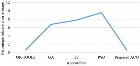
The percentage relative error average for the suggested ACO, OR-Tools, GA, TS, and PSO is displayed in Figure 4. The suggested ACO's percentage relative error average is just 0.67%, indicating an excellent estimation to the JSSP optimum.
Figure 4. Relative error average by approaches
Our proposed ACO is applied to address a JSSP in the pharmaceutical industry at the BIOCARE.
6.1 Company presentation
Pharmaceutical Industry BIOCARE the parent company of the BIOCARE Group, a dynamic Algerian conglomerate with a strong corporate culture, structured into several subsidiaries operating in the pharmaceutical domain.
The industrial zone comprises various dedicated structures, designed with a layout that facilitates the flow of raw materials and finished products. Notably, there is an administrative building, two production zones, Alpha (non-Betalactam) and Beta (Betalactam), a quality control laboratory, and a storage hangar for products.
Emphasis is placed on the pharmaceutical quality of raw materials, with a stringent selection of suppliers and multiple checks (physicochemical and microbiological) from reception to finished products.
All operators undergo regular training on manufacturing processes and associated risks, enabling them to master all procedures and parameters during various phases (production, control, cleaning, maintenance, etc.).
At BIOCARE, the two major industrial stages in the production of a medication are the manufacturing process and the packaging process.
6.2 Manufacturing process
Figure 5 shows the steps of the manufacturing process at BIOCARE.
6.3 Packaging process
Figure 6 shows the steps of the packaging process at BIOCARE.
6.4 Product flow in the pharmaceutical industry BIOCARE
In the pharmaceutical industry at BIOCARE, a multitude of products exists. The one-week schedule proposed by the company involves the production of 4 different types of medications, with each type having a set of batches manufactured. Table 3 lists the medications considered in the schedule, representing the jobs.
Figure 5. The steps of the manufacturing process
Figure 6. The steps of the packaging process
Table 3. The jobs
|
Job |
J1 |
J2 |
J3 |
J4 |
|
Products |
Trimebutine |
Diaglinide 2 mg |
Antage 20 mg |
Biovex |
6.5 Machine at the manufacturing line in the pharmaceutical industry BIOCARE
The manufacturing workshop at BIOCARE consists of 9 machines (M1, M2, ..., M9), representing the production chain required to carry out the previously mentioned 4 jobs. Table 4 illustrates the breakdown of machines in the workshop. This data is provided by the company.
6.6 Product flow at the machines in the manufacturing workshop in the pharmaceutical industry BIOCARE
The production of a medication (job) involves the use of multiple machines, necessitating the division of each job into a set of operations equal to the number of machines required in its manufacturing process, and the assignment of each operation to a machine. Each operation is processed by a predetermined machine for a predetermined duration. Table 5 illustrates the allocation of operations on the machines. In Table 5, Pij indicates the processing times of each operation j of job i on machine k, including the cleaning time. Indeed, at the end of each operation, it is necessary to clean the machine and the premises before they are used again for another type of medication. These data are provided by the company.
Table 4. Machine allocation in the workshop
|
Workshop |
Machine Symbol |
Machine Description |
|
Manufacturing |
M1 |
Weighing |
|
M2 |
Granulator 250℃ |
|
|
M3 |
Tablet Press |
|
|
M4 |
Coating Machine |
|
|
M5 |
Blister Packaging |
|
|
M6 |
Boxing |
|
|
M7 |
Mixing |
|
|
M8 |
Encapsulation |
|
|
|
M9 |
Bagging |
Table 5. Job flow on the machine
|
Job |
Workshop |
Operation |
Machine Symbol |
Machine Description |
$\boldsymbol{P}_{i j}$ (hours) |
|
J1 |
Manufacturing |
O11 |
M1 |
Weighing |
4 |
|
O12 |
M2 |
Granulator 250°C |
7 |
||
|
O13 |
M3 |
Tablet Press |
15 |
||
|
O14 |
M4 |
Coating Machine |
5 |
||
|
O15 |
M5 |
Blister Packaging |
12 |
||
|
O16 |
M6 |
Boxing |
16 |
||
|
J2 |
Manufacturing |
O21 |
M1 |
Weighing |
6 |
|
O22 |
M7 |
Mixing |
3 |
||
|
O23 |
M3 |
Tablet Press |
48 |
||
|
O24 |
M5 |
Blister Packaging |
32 |
||
|
O25 |
M6 |
Boxing |
20 |
||
|
J3 |
Manufacturing |
O31 |
M8 |
Encapsulation |
72 |
|
O32 |
M5 |
Blister Packaging |
80 |
||
|
J4 |
Manufacturing |
O41 |
M1 |
Weighing |
5 |
|
O42 |
M2 |
Granulator 250°C |
8 |
||
|
O43 |
M9 |
Bagging |
40 |
||
|
O44 |
M6 |
Boxing |
16 |
Figure 7. The data for the job shop BIOCARE
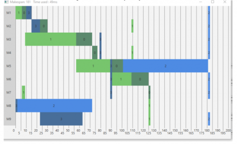
Figure 8. Makespan and Gantt diagram BIOCARE
6.7 Application of the suggested ACO to address the BIOCARE JSSP
We executed the pharmaceutical scheduling problem using our proposed ACO algorithm. The planning period considered by BIOCARE corresponds to one week. Production operates 6 days out of 7, with two alternating teams to ensure production. Since these teams have a one-hour break, the total production time per day is 2×(8−1) =2×7=14 hours. It is considered that a working day is equivalent to 14 hours, and thus, the proposed schedule lasts for 14×6 hours, which is 84 hours.
The JSSP involving instances (4×9) for the 4 jobs and 9 machines that constitute the manufacturing workshop is solved using the suggested ACO (see Figure 7). The makespan obtained is 181 hours, as illustrated in Figure 8. The goal has been achieved. In fact, compared to the schedule proposed by the company, approximately 3 hours have been saved. While this saved time may seem relatively short, it's important to consider that the planning period is quite brief (one week). Furthermore, in addition to saving time in completing all the scheduled jobs, our schedule also appears to provide more available time slots for tasks beyond the original plan. This improvement encompasses not only the total duration but also machine availability.
The goal of this work is to solve a JSSP using ACO, a bioinspired intelligence technique and its application to a real-life case within the pharmaceutical products laboratory (BIOCARE). The adapted ACO was compared to other approaches for solving JSSP to demonstrate its effectiveness. The competitiveness of the developed algorithm ACO has been demonstrated by its ability to discover excellent solutions for JSSP in a short time. During the experiments, the adapted ACO and the other approaches succeeded to find the makespan for several benchmark examples. However, the performance was limited for large-scale problems. The adapted ACO turned out to be better at addressing large JSSP with an execution time that increases with the number of jobs. turned out to be better at addressing big JSSP. It achieved this with an average percentage relative error of only 0.67%, although its execution time increased with the execution time increasing as the number of tasks and the number of ants increase, which represents a challenge and drawback of the ACO.
Notably, when we applied the implemented ACO to the pharmaceutical company BIOCARE, an important rise in planning efficiency in contrast to the company's existing techniques, resulting in an approximate 3-hour improvement in their weekly planning.
In general, we conclude that ACO could be successfully applied to real-world industrial problems.
As perspective, we plan to apply the proposed ACO to identify the best solutions for the large-scale instances in other industries.
Also, to harness high-performance computing technologies and parallelism. By employing hybrid metaheuristics, which combine ACO with other optimization techniques to search for optimal solutions in complex search spaces while reducing computation time.
|
JSSP |
Job Shop Scheduling Problem |
|
ACO |
Ant Colony Optimization |
|
ASP |
Answer Set Programming |
|
TS |
Tabu Search |
|
GA |
Genetic Algorithm |
|
PSO |
Particle Swarm Optimization |
|
Greek symbols |
|
|
$\alpha$ |
Impact of pheromone |
|
$\beta$ |
Impact of desirability |
|
$\rho$ |
Rate of evaporation of the pheromone |
|
$\tau$ |
Pheromone amount |
|
$\eta$ |
Desirability |
[1] Brucker, P., Jurisch, B. (1993). A new lower bound for the job-shop scheduling problem. European Journal of Operational Research, 64(2): 156-167. https://doi.org/10.1016/0377-2217(93)90174-L
[2] Brucker, P., Urisch, B., Sievers, B.A (1994). Branch and bound algorithm for job shop scheduling problem. Discret. Appl. Math., 49: 107-127.
[3] Baptiste, P., Flamini, M., Sourd, F. (2008). Lagrangian bounds for just-in-time job shop scheduling. Computers & Operations Research, 35(3): 906-915. https://doi.org/10.1016/j.cor.2006.05.009
[4] Dovier, A., Formisano, A., Pontelli, E. (2005). A comparison of CLP (FD) and ASP solutions to NP-complete problems. In: Gabbrielli, M., Gupta, G. (eds) Logic Programming. ICLP 2005. Lecture Notes in Computer Science, vol 3668. Springer, Berlin, Heidelberg. https://doi.org/10.1007/11562931_8
[5] Brewka, G., Eiter, T., Truszczyński, M. (2011). Answer set programming at a glance. Communications of the ACM, 54(12): 92-103. https://doi.org/10.1145/2043174.2043195
[6] Falkner, A., Friedrich, G., Schekotihin, K., Taupe, R., Teppan, E.C. (2018). Industrial applications of answer set programming. KI-Künstliche Intelligenz, 32(2-3): 165-176. https://doi.org/10.1007/s13218-018-0548-6
[7] Dal Palù, A., Dovier, A., Formisano, A., Pontelli, E. (2018). Exploring life: Answer set programming in bioinformatics. Declarative Logic Programming: Theory, Systems, and Applications, pp. 359-412. https://doi.org/10.1145/3191315.3191323
[8] Nowicki, E., Smutnicki, C. (1996). A fast taboo search algorithm for the job shop problem. Management Science, 42(6): 797-813. https://doi.org/10.1287/mnsc.42.6.797
[9] Taillard, E.D. (1994). Parallel taboo search techniques for the job shop scheduling problem ORSA Journal on Computing, 6(2): 108-117. https://doi.org/10.1287/ijoc.6.2.108
[10] Dell’Amico, M., Trubian, M. (1993). Applying tabu search to the job-shop scheduling problem. Annals of Operations Research, 41(3): 231-252. https://doi.org/10.1007/BF02023076
[11] Nowicki, E., Smutnicki, C. (2005). An advanced tabu search algorithm for the job shop problem. Journal of Scheduling, 8(2): 145-159. https://doi.org/10.1007/s10951-005-6364-5
[12] Leusin, M.E, Frazzon, E.M., Uriona Maldonado, M., Kück, M., Freitag, M. (2018). Solving the job-shop scheduling problem in the industry 4.0 era. Technologies, 6(4): 107. https://doi.org/10.3390/technologies6040107
[13] Çaliş, B., Bulkan, S. (2015). A research survey: Review of AI solution strategies of job shop scheduling problem. Journal of Intelligent Manufacturing, 26: 961-973. https://doi.org/10.1007/s10845-013-0837-8
[14] Matrenin, P.V., Manusov, V.Z. (2022) The cyclic job-shop scheduling problem: The new subclass of the job-shop problem and applying the simulated annealing to solve it. In Proceedings of the IEEE 2nd International Conference on Industrial Engineering, Applications and Manufacturing (ICIEAM), Chelyabinsk, Russia, pp. 1-5. https;//doi.org/10.1109/ICIEAM.2016.7911676
[15] Asadzadeh, L. (2015). A local search genetic algorithm for the job shop scheduling problem with intelligent agents. Computers & Industrial Engineering, 85: 376-383. https://doi.org/10.1016/j.cie.2015.04.006
[16] Kundakcı, N., Kulak, O. (2016). Hybrid genetic algorithms for minimizing makespan in dynamic job shop scheduling problem. Computers & Industrial Engineering, 96: 31-51. https://doi.org/10.1016/j.cie.2016.03.011
[17] Gao, J., Gen, M., Sun, L.Y., Zhao, X. (2007). Hybrid of genetic algorithm and bottleneck shifting for multiobjective flexible job shop scheduling problems. Computers & Industrial Engineering, 53: 149-162. https://doi.org/10.1016/j.cie.2007.04.010
[18] Matrenin, P.V., Sekaev, V.G. (2015). Particle Swarm optimization with velocity restriction and evolutionary parameters selection for scheduling problem. In Proceedings of the IEEE International Siberian Conference on Control and Communications (SIBCON), Omsk, Russia, pp. 1-5. https://doi.org/10.1109/SIBCON.2015.7147143
[19] Liu, B., Wang, L., Jin, Y.H. (2008). An effective hybrid PSO-based algorithm for flow shop scheduling with limited buffers. Computers & Operations Research, 35(9): 2791-2806. https://doi.org/10.1016/j.cor.2006.12.013
[20] Xiang, W., Lee, H.P. (2008). Ant colony intelligence in multi-agent dynamic manufacturing scheduling. Engineering Applications of Artificial Intelligence, 21(1): 73-85. https://doi.org/10.1016/j.engappai.2007.03.008
[21] Wang, L., Cai, J., Li, M., Liu, Z. (2017). Flexible job shop scheduling problem using an improved ant colony optimization. Scientific Programming, 2017: 9016303. https://doi.org/10.1155/2017/9016303
[22] Liao, C.J., Huang, K.L. (2008). Ant colony optimization combined with taboo search for the job shop scheduling problem. Computers and Operations Research, 35(4): 1030-1046. https;//doi.org/10.1016/j.cor.2006.07.003
[23] Matrenin, P., Myasnichenko, V., Sdobnyakov, N., Sokolov, S., Fidanova, S., Kirillov, L., Mikhov, R. (2021). Generalized swarm intelligence algorithms with domain-specific heuristics. IAES International Journal of Artificial Intelligence (IJ-AI), 10(1): 157-165. http://doi.org/10.11591/ijai.v10.i1.pp157-165
[24] Ponnambalam, S.G., Jawahar, N., Girish, B.S. (2009). Giffler and Thompson procedure based genetic algorithms for scheduling job shops. In: Chakraborty, U.K. (eds) Computational Intelligence in Flow Shop and Job Shop Scheduling. Studies in Computational Intelligence, vol 230. Springer, Berlin, Heidelberg. https://doi.org/10.1007/978-3-642-02836-6_8
[25] Fisher, H., Thompson, G.L. (1963). Probabilistic learning combinations of local job shop scheduling rules. In: Industrial Scheduling. Sous la dir. de J.F. Muth et G.L. Thompson. Prentice Hall, pp. 225-251.
[26] Lawrence, S. (1984). Resource constrained project scheduling: An experimental investigation of heuristic scheduling techniques (supplement). Graduate School of Industrial Administration, Carnegie-Mellon University.
[27] Applegate, D., Cook, W. (1991). A computational study of job-shop scheduling. ORSA Journal of Computing, 3(2): 149-156. https://doi.org/10.1287/ijoc.3.2.149
[28] Li, Y.T., Manner, R., Manderick, B. (1992). A genetic algorithm applicable to large-scale job-shop instances. In Parallel Problem Solving from Nature, pp. 281-290. North-Holland.
[29] Taillard, E.D. (1993). Benchmarks for basic scheduling problems. European Journal of Operational Research, 64(2): 278-285. https://doi.org/10.1016/0377-2217(93)90182-M
[30] Adams, J., Balas, E., Zawack, D. (1988). The shifting bottleneck procedure for job shop scheduling. Management Science, 34(3): 391-401. https://doi.org/10.1287/mnsc.34.3.391