Attarid K. Ahmed*![]() | Huthaifa Al-Khazraji
| Huthaifa Al-Khazraji![]()
© 2023 IIETA. This article is published by IIETA and is licensed under the CC BY 4.0 license (http://creativecommons.org/licenses/by/4.0/).
OPEN ACCESS
This study conducts a comprehensive examination of the nonlinear propeller pendulum system's angular position control, utilizing three distinct control strategies: Proportional-Integral-Derivative (PID) controller, State Feedback (SF) controller, and Sliding Mode Control (SMC). In order to optimize the performance of each controller, Gorilla Troops Optimization (GTO) is employed to identify the optimal value of the controllers' design parameters. The dynamics of the system under each controller are simulated via MATLAB software, and the performance of the controlled system is quantitatively assessed utilizing the Integral Time of Absolute Error (ITAE). The resilience of the controllers under uncertainties is evaluated by introducing an external disturbance to the system. Simulation results indicate that the SMC, tuned by GTO, exceeds the performance of the other controllers in reducing the settling time, eliminating maximum overshoot, and minimizing the ITAE index. Moreover, under external disturbance, the SMC tuned by GTO demonstrates superior robustness compared to other controllers.
nonlinear system, propeller pendulum system, PID controller, state feedback controller, sliding mode control, swarm optimization, gorilla troops optimization
A propeller pendulum system is a type of nonlinear dynamic system that integrates a propeller with a pendulum. The propeller is motorized to generate a thrust force at the end of a pendulum rod such that the pendulum can lift up and down [1]. The simple pendulum system is a standard topic in most physics educational courses because it includes some physical subjects including the simple harmonic motion, the acceleration of gravity, and the center of mass [2]. Besides, the system is considered a nonlinear model that can be used in the education of mechatronics, control, and mechanical engineering to explain the system dynamics and methods of controller design [3]. Moreover, the propeller pendulum system can be used to model the take-off and landing of aircraft [4]. Therefore, modeling and controlling propeller pendulum system are gained high attention as a research topic.
Various control methods have been applied to control and stabilize the propeller pendulum at any desired position such as Proportional-Integral-Derivative (PID) controller [2, 5], Linear Quadratic Regulator (LQR) [6], Quadratic Dynamic Matrix Control (QDMC) [7], Fuzzy PID controller [1], Sliding Mode Control (SMC) [8], Adaptive Super-Twisting SMC (ASTSMC) [4] and Adaptive Backstepping Control (ABSC) [3].
With the substantial improvement in the capabilities of swarm optimization algorithms such as the ability in handling multivariate, high dimensional problems and easy implementation, these algorithms have been successfully utilized in different fields of applications [9]. Among these applications, they combined with classical and modern controllers for further improvement in the performance of the controller. In this direction, this paper proposes three control strategies including the Proportional-Integral-Derivative (PID) controller, State Feedback (SF) controller, and Sliding Mode Control (SMC) to control the angular position of the nonlinear propeller pendulum. For further enhancement of the proposed three controllers, this study has employed Gorilla Troops Optimization (GTO) to find the optimal value of the design parameters of the proposed controllers. The GTO algorithm is inspired by the social behavior and daily activity such as taking rest, traveling, and eating of gorilla troops.
The novelty of the current work as compared to previous studies can be stated as follows. PID and SF controllers are commonly used to improve the dynamic performance of the linear system. For such systems, the classical control methods such as Ziegler-Nichols or root locus for PID controller and pole placement or LQR for SF controller can be used to determine the design parameters of the controllers. However, for nonlinear systems, the system is often linearized about an operation point, and then the SF and PID controllers are applied. As an example of using the linearized model of a propeller pendulum, Mohammadbagheri and Yaghoobi [2] used Ziegler and Nichols method to tune the PID controller. The same strategy has been used by Günel and Ankarah [5]. In Günel's and Ankarah’s [5] work, the Genetic Algorithm (GA) and Particle Swarm Optimization (PSO) are employed to tune the design variables of the PID controller. In the context of the SF controller, Farmanbordar et al. [6] used the LQR approach based on a linearized model of the propeller pendulum. However, these papers presented an approach that can be successfully utilized for systems with a small region of operation. To avoid this restriction, Taskin [1] proposed a Fuzzy PID controller for the nonlinear propeller pendulum system. The design variables of the PID controller are calculated by a fuzzy logic unit. Unlike these works, this paper proposed the recent swarm optimization GTO as a method to find the optimal value of the design parameters of the PID and SF controllers directly based on the nonlinear propeller pendulum system.
In terms of SMC, there are two works in the literature that are considered SMC as the controller of the propeller pendulum system. Kizmaz et al. [8] used a linearized model of the propeller pendulum system. However, in the present work, the SMC is designed based on the nonlinear dynamics of the propeller pendulum system. In addition, the chattering problem in the voltage control signal was very high. The second work on the SMC was presented by Al-Qassar et al. [4]. Al-Qassar et al. [4] adopted the Super-Twisting approach to cope with the chattering problem in the SMC. The present paper utilizes a different approach based on the power rate reaching law method to avoid the chattering problem and control the nonlinear propeller pendulum system.
To end this, the paper is organized as follows. The mathematical model of the nonlinear propeller pendulum system is formulated in Section 2. Section 3 presents the procedure to design the proposed controllers. In Section 4, the GTO algorithm is described. The simulation outcomes of the nonlinear propeller pendulum system with each controller are discussed in Section 5. The conclusion of this paper is summarized in Section 6.
To effectively control the propeller pendulum system, an accurate mathematical model of the dynamics of the system is first obtained. Figure 1 shows the schematic diagram of the propeller pendulum system.
Figure 1. Propeller pendulum system
As indicated in the Figure 1, there is a DC motor with a propeller is attached at the end of the arm. The input voltage of the DC motor is the control input u(t) and the angle position $\theta(\mathrm{t})$ between the arm and vertical axis is the control variable. After applied voltage to the DC motor, the propeller spins and generates torque $\mathrm{T}_{\mathrm{m}}(\mathrm{t})$ to move the arm with an angular speed $\dot{\theta}(\mathrm{t})$ and an angular acceleration $\ddot{\theta}(\mathrm{t})$. Based on Newton’s, the equation of motion of the propeller pendulum is given by [2]:
$J \ddot{\theta}(t)+c \dot{\theta}(t)+\operatorname{mgd}(\sin \theta(t))=T_m(t)$ (1)
where, J, C, m, g and d are inertia of moment, viscous damping coefficient, mass of propeller, acceleration of gravity, distance from suspending point to the mass center respectively.
The relationship between the input voltage and the torque produced from the DC motor is formulated as [2, 4]:
$\mathrm{T}_{\mathrm{m}}(\mathrm{t})=\mathrm{K}_{\mathrm{m}} \mathrm{u}(\mathrm{t})$ (2)
where, $\mathrm{K}_{\mathrm{m}}$ refers to the constant of the DC motor of the propeller.
Substitute Eq. (2) into Eq. (1) gives:
$J \ddot{\theta}(\mathrm{t})+\mathrm{c} \dot{\theta}(\mathrm{t})+\operatorname{mgd}(\sin \theta(\mathrm{t}))=\mathrm{K}_{\mathrm{m}} \mathrm{u}(\mathrm{t})$ (3)
Rearrange Eq. (3) obtains:
$\ddot{\theta}(\mathrm{t})=\frac{-\mathrm{C} \dot{\theta}(\mathrm{t})-\operatorname{mgd}(\sin \theta(\mathrm{t}))+\mathrm{K}_{\mathrm{m}} \mathrm{u}(\mathrm{t})}{J}$ (4)
Let $x_1(t)$ represent the angle position $\theta(\mathrm{t})$, and $x_2(t)$ represent the angle velocity $\dot{\theta}(\mathrm{t})$. The dynamics of the propeller pendulum system are given by the following differential equations:
$\dot{\mathrm{x}}_1(\mathrm{t})=\mathrm{x}_2(2)$ (5)
$\dot{\mathrm{x}}_2(\mathrm{t})=\frac{-\mathrm{Cx}_2(\mathrm{t})-\mathrm{mgd}\left(\sin x _1(\mathrm{t})\right)+\mathrm{K}_{\mathrm{m}} \mathrm{u}(\mathrm{t})}{\mathrm{J}}$ (6)
In this paper, three feedback control loop mechanisms named Proportional-Integral-Derivative (PID) controller, State Feedback (SF) controller, and Sliding Mode Control (SMC) are used to control the angular position of the nonlinear propeller pendulum system. SMC can be directly applied to a nonlinear dynamic system. However, the PID and SF controller are commonly used for linear systems where classical control methods such as Ziegler-Nichols for PID controller and pole placement for SF controller can be used to determine the design parameters of the controllers. However, for nonlinear system, the system need to be linearized about an operation point, and then the SF and PID controllers are applied. This approach can be successful works for systems with a small region of operation. To avoid this restriction, the swarm optimization is used to tune the design parameters of the PID and SF controllers for the nonlinear propeller pendulum system.
3.1 PID controller
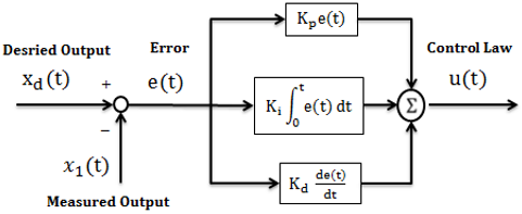
PID controllers are a type of feedback control loop mechanism that is commonly employed in industrial control systems. The control law u(t) in the PID controller is determined based on the error e(t) between the measured output $\mathrm{x}_1(\mathrm{t})$ and the desired output $\mathrm{x}_d(\mathrm{t})$ [10]. It has three terms. The proportional terms adjust u(t) based on the weighted gain $\mathrm{K}_{\mathrm{p}}$ of the present e(t). The integral terms adjust the u(t) based on the weighted gain $\mathrm{K}_{\mathrm{i}}$ of the integration of e(t). The derivative terms adjust u(t) based on the weighted gain $\mathrm{K}_{\mathrm{d}}$ of the rate of change of e(t). The final response of the PID controller is based on the summation of these three terms. The control law of the PID controller is given by studies [11, 12]:
$u(t)=K_p e(t)+K_i \int_0^t e(t) d t+K_d \frac{d e(t)}{d t}$ (7)
Figure 2 shows the general block diagram of the PID controller.
Figure 2. PID block diagram
3.2 State feedback controller
State feedback controllers are widely used in various control applications such as set-point tracking and disturbance rejection. The state feedback controller is a control mechanism used to place the closed-loop poles of a plant in desired locations in the s-plane. As the eigenvalues of the system is based on the pole location, the SF controller is control the characteristics of the response of the system. In order to apply the SF controller, the system needs to be controllable and. The control law u(t) in the SF controller is determined based on the difference between the forward-weighted gain $\mathrm{K}_{\mathrm{x}_{\mathrm{d}}}$ of the desired output $x_d(t)$ and feedback-weighted gains $\mathrm{K}_{\mathrm{x}_1}$ and $\mathrm{K}_{\mathrm{x}_2}$ of the states $\left(\mathrm{x}_1, \mathrm{x}_2\right)$ of the system. In the SF controller, the choice of the design variables ($\mathrm{K}_{\mathrm{x}_{\mathrm{d}}}, \mathrm{K}_{\mathrm{x}_1}$, and $\mathrm{K}_{\mathrm{x}_2}$) is very importance and affects the system performance. The control law of the SF controller is given by [13]:
$\mathrm{u}(\mathrm{t})=\mathrm{K}_{\mathrm{x}_{\mathrm{d}}} \mathrm{x}_{\mathrm{d}}(\mathrm{t})-\left[\begin{array}{l}\mathrm{K}_{\mathrm{x}_1} \\ \mathrm{~K}_{\mathrm{x}_2}\end{array}\right]\left[\mathrm{x}_1(\mathrm{t}) \mathrm{x}_2(\mathrm{t})\right]$ (8)
Figure 3 shows the general block diagram of the SF controller.
Figure 3. SF block diagram
3.3 Sliding mode control
SMC is a well-known as robustness and systematic design controller. It has two stages. Defining the sliding surfaces for the required performance is the first stage. Then, keeping the system on the sliding surface is the second stage [14]. The sliding surface is defined as:
$\mathrm{s}(\mathrm{t})=\dot{\mathrm{e}}(\mathrm{t})+\mathrm{a}_{\mathrm{smc}} \mathrm{e}(\mathrm{t})$ (9)
where, e(t) is the error between the measured output $x_1(t)$ and the desired output $x_d(t)$, and $\mathrm{a}_{\mathrm{smc}}>0$ is a tuning parameters.
Taking the first derivative of the sliding surface yields:
$\begin{aligned} \dot{\mathrm{s}}(\mathrm{t})=\ddot{\mathrm{e}}(\mathrm{t})+\mathrm{a}_{\mathrm{smc}} \dot{\mathrm{e}}(\mathrm{t}) =\ddot{\mathrm{x}}_{\mathrm{d}}(\mathrm{t})-\dot{\mathrm{x}}_2(\mathrm{t})+\mathrm{a}_{s m c} \dot{\mathrm{x}}_{\mathrm{d}}(\mathrm{t}) -\mathrm{a}_{s m c} \mathrm{x}_2(\mathrm{t})\end{aligned}$ (10)
Substitute $\dot{x}_2(t)$ from Eq. (6) into Eq. (10) obtains:
$\begin{aligned} & \dot{\mathrm{s}}(\mathrm{t}) =\ddot{\mathrm{x}}_{\mathrm{d}}(\mathrm{t})+\mathrm{a}_{\mathrm{smc}} \dot{\mathrm{x}}_{\mathrm{d}}(\mathrm{t}) -\left(\frac{-\mathrm{Cx}_2(\mathrm{t})-\operatorname{mgd}\left(\sin \mathrm{x}_1(\mathrm{t})\right)+\mathrm{K}_{\mathrm{m}} \mathrm{u}(\mathrm{t})}{\mathrm{J}}\right) -\mathrm{a}_{\mathrm{smc} \mathrm{x}_2(\mathrm{t})}\end{aligned}$ (11)
The second part of the control law in the SMC is the switching control. Switching control appears in the SMC as a discontinuous control law that makes the system slide on the surface [15]. To ensure that the system is sliding on the surface, the first derivative of the sliding surface should be equal to the switching control. Therefore, the switching control needs to select properly to avoid the chattering phenomena that exist in SMC [16]. In this direction, the power rate reaching law is used for the switching control which is given by the study [17]:
$\dot{s}(\mathrm{t})=-\mathrm{k}_{\mathrm{smc}}|\mathrm{s}(\mathrm{t})|^\gamma \mathrm{sgn}(\mathrm{s}(\mathrm{t}))$ (12)
where, sgn is sign function, $\mathrm{k}_{\mathrm{smc}}$ is adjusted parameter >0, γ is adjusted parameter between [0,1]. The final u(t) is determined by setting Eq. (11) and is equal to Eq. (12) as given:
$\begin{aligned} & \ddot{\mathrm{x}}_{\mathrm{d}}(\mathrm{t})+\mathrm{a}_{\mathrm{smc}} \dot{\mathrm{x}}_{\mathrm{d}}(\mathrm{t}) -\left(\frac{-\mathrm{Cx}_2(\mathrm{t})-\operatorname{mgd}\left(\operatorname{sinx}_1(\mathrm{t})\right)+\mathrm{K}_{\mathrm{m}} \mathrm{u}(\mathrm{t})}{\mathrm{J}}\right) -\mathrm{a}_{\mathrm{smc}} \mathrm{x}_2(\mathrm{t})=-\mathrm{k}_{\mathrm{smc}}|\mathrm{s}|^\gamma \operatorname{sgn}(\mathrm{s})\end{aligned}$ (13)
Rearrange Eq. (13) to find the control law of the SMC as:
$\begin{aligned} \mathrm{u}(\mathrm{t})=\frac{\mathrm{J}}{\mathrm{K}_{\mathrm{m}}}\left(\ddot{\mathrm{x}}_{\mathrm{d}}(\mathrm{t})\right. & +\mathrm{a}_{\mathrm{smc}} \dot{\mathrm{x}}_{\mathrm{d}}(\mathrm{t})+\mathrm{k}_{\mathrm{smc}}|\mathrm{s}|^\gamma \mathrm{sgn}(\mathrm{s}) -\mathrm{a}_{\mathrm{smc} \mathrm{x}_2(\mathrm{t})} \left.+\frac{\mathrm{Cx}_2(\mathrm{t})+\operatorname{mgd}\left(\operatorname{sinx}_1(\mathrm{t})\right)}{J}\right)\end{aligned}$ (14)
Figure 4 shows the general block diagram of the SMC controller.
Figure 4. SMC block diagram
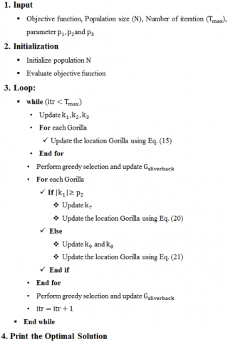
Swarm optimization is a population-based algorithm used to solve optimization problems and seek optimal solutions. Due to their simplicity, ease of implementation and reasonable time to find the solution, these algorithms become very popular for solving different optimization problems. Most of these algorithms are natural-based-algorithm [18, 19]. In this paper, one of the recent swarm optimization, named Gorilla Troops Optimization, is used to solve the tuning problem of the design variable of the controllers proposed to control the propeller pendulum system. Gorilla Troops Optimization (GTO) is a swarm optimization developed by Abdollahzadeh et al. [20] in 2021. The algorithm is inspired by the social behavior and daily activity such as taking rest, traveling, and eating of gorilla troops. They live in a group called troops. The adult male gorilla is named Silverback [21]. Abdollahzadeh et al. [20] formulated the natural behavior of gorilla troops by five equations. The pseudo-code of the GTO algorithm is given in Figure 5. The exploration search is described by three equations including move to unknown places, move to known places, and move to another gorilla. To maintain a proper balance between these mechanisms to update the position of gorillas, it is assumed that there is a probability of 50% to choose between them. These three equations are given in Eq. (15).
$\begin{aligned} & \mathrm{GX}(\mathrm{itr}+1) =\left\{\begin{array}{cr}\mathrm{LB}+\mathrm{r}_1(\mathrm{UB}-\mathrm{LB}), & \text { rand }<\mathrm{p}_1 \\ \mathrm{GR}(\mathrm{itr})\left(\mathrm{r}_2-\mathrm{k}_1\right)+\mathrm{k}_2 \mathrm{k}_3, & \text { rand } \geq 0.5 \\ \mathrm{GX}(\mathrm{itr})-\mathrm{k}_2\left(\begin{array}{c}\mathrm{k}_2(\mathrm{GX}(\mathrm{itr})-\mathrm{GR}(\mathrm{itr})) \\ +\mathrm{r}_3(\mathrm{GX}(\mathrm{itr})-\mathrm{GR}(\mathrm{itr}))\end{array}\right) \\ \text { rand }<0.5\end{array},\right. \\ & \end{aligned}$ (15)
where, LB is lower bound, UB is upper bound, itr is current iteration, GX(itr+1) is new solution, GR(itr) is solution selected randomly, GX(itr) is current solution, r1, r2 and r3 are random number between [0,1], p1 is coefficients determined by the user between [0,1], coefficientsk1, k2, k3 and k4 are computed as follows [22]:
$\mathrm{k}_1=\mathrm{k}_4\left(1-\frac{\mathrm{itr}}{\mathrm{T}_{\max }}\right)$ (16)
$\mathrm{k}_2=\mathrm{k}_1 \mathrm{k}_5$ (17)
$\mathrm{k}_3=\mathrm{k}_6 \mathrm{GX}(\mathrm{itr})$ (18)
$\mathrm{k}_4=\cos \left(2 \mathrm{r}_4\right)+1$ (19)
where, Tmax is maximum iteration, r4 is random number between [0,1], k5 is random number between [-1,1], k6 is random number between $\left[-\mathrm{k}_1, \mathrm{k}_1\right]$.
On the other hand, the exploitation search is described by two equations including following the silverback and the competition for adult females. Based on the coefficients $\mathrm{k}_1$, the gorillas either follow the silverback or competition with adult females. If $\mathrm{k}_1 \geq \mathrm{p}_2$, gorillas follow the silverback based on Eq. (20). On the other hand, if $\mathrm{k}_1<\mathrm{p}_2$, gorillas compete for adult females based on Eq. (21), where $\mathrm{p}_2$ is determined by the user [20].
$\begin{aligned} \mathrm{GX}(\mathrm{itr}+1)=\mathrm{GX} & (\mathrm{itr}) +\mathrm{k}_1 \mathrm{k}_7\left(\mathrm{GX}(\mathrm{itr})-\mathrm{G}_{\text {sliverbark }}\right)\end{aligned}$ (20)
$\begin{aligned} \mathrm{GX}(\mathrm{itr}+1)=\mathrm{G}_{\text {sliverback }} -\mathrm{k}_9 \mathrm{k}_8\left(\mathrm{G}_{\text {sliverback }}-\mathrm{GX}(\mathrm{itr})\right)\end{aligned}$ (21)
Coefficients k7, k8, and k9 are computed as follows [22]:
$\mathrm{k}_7=\left(\left|\frac{1}{\mathrm{~N}} \sum_{\mathrm{j}=1}^{\mathrm{N}} \mathrm{GX}_{\mathrm{i}}(\mathrm{itr})\right|^{\mathrm{gn}}\right)^{\frac{1}{\mathrm{~g}_{\mathrm{n}}}}$ (22)
$\mathrm{g}_{\mathrm{n}}=2^{\mathrm{k}_2}$ (23)
$\mathrm{k}_{\mathrm{8}}=\mathrm{p}_3 \mathrm{k}_{10}$ (24)
$\mathrm{k}_9=2 \mathrm{r}_5-1$ (25)
$\mathrm{k}_{10}= \begin{cases}\mathrm{rn}_1, & \text { rand } \geq 0.5 \\ \mathrm{rn}_2, & \text { rand }<0.5\end{cases}$ (26)
where, N is the population size, $\mathrm{p}_3$ is coefficients determined by the user, $\mathrm{p}_5$ is a random number between [0,1], $r n_1$ is random number between [0,N], $r n_2$ is random number.
Figure 5. Pseudo-code of the GTO algorithm
In this section, the simulations of controlling the nonlinear propeller pendulum system using three control structures, PID controller, SF controller, and SMC, are presented. The objective of the controller is to make the system follow a desired angular position. The simulation experiments and performance evaluation are conducted using MATLAB software. The Runge Kutta (ode45 in MATLAB) method has been used to solve the differential equations in the simulation. The dynamics of the propeller pendulum system that is described by Eq. (5) and Eq. (6) are used in the simulation. The parameters of the system are given in Table 1 [4]. It must be pointed out that, the input voltage to the DC motor of the propeller pendulum system is saturated by ±30 V.
Table 1. Parameters of the propeller pendulum system
|
Parameter and Symbol |
Value and Unit |
|
Moment of inertia $(\mathrm{J})$ |
0.0106 $\mathit{kg} \cdot \mathit{m}^2$ |
|
Viscous damping coefficient $(\mathrm{C})$ |
0.0076 Nms/rad |
|
Mass of propeller $(\mathrm{m})$ |
0.36 $\mathit{kg}$ |
|
Acceleration due to gravity $(\mathrm{g})$ |
9.81 $\mathit{m} / \mathit{s}^2$ |
|
Distance from suspending point to the mass center $(\mathrm{d})$ |
0.03 $m$ |
|
Motor constant $\mathrm{K}_{\mathrm{m}}$ |
0.0296 |
To ensure the optimal performance of each controller, the GTO is employed to tune the design parameters of each controller. The performance of the PID controller is optimized by tuning the adjusted parameters (Kp, Ki, and Kd) of the control law that is given in Eq. (7). In the same way, the performance of the SF controller is optimized by tuning the adjusted parameters $\left(\mathrm{K}_{\mathrm{x}_{\mathrm{d}}}, \mathrm{K}_{\mathrm{x}_1}\right.$ and $\left.\mathrm{K}_{\mathrm{x}_2}\right)$ of the control law that is given in Eq. (8). Besides, the performance of the SMC is optimized by tuning the adjusted parameters ($\mathrm{K}_{\mathrm{smc}}$, $a_{s m c}$ and $\gamma$) of the control law that is given in Eq. (14). The Integral Time of Absolute Errors (ITAE) as given in Eq. (27) [23] is used to evaluate the controlled system.
$\operatorname{ITAE}=\int_{t=0}^{\mathrm{t}=\mathrm{t}_{\mathrm{sim}}} \mathrm{t}|\mathrm{e}(\mathrm{t})| \mathrm{dt}$ (27)
where, $t_{\operatorname{sim}}$ is the simulation time.
The parameters of the GTO are listed in Table 2. The convergence of GTO for tuning the three controllers is shown in Figure 6.
Figure 6. Convergence of GTO for the proposed controllers
The values of the designed parameters of the PID controller, SF controller, and SMC are given in Table 3. The convergence of GTO for the proposed controllers is shown in Figure 6. The control signals of the proposed controllers are shown in Figure 7.
Table 2. Algorithm parameters of GTO
|
Parameter |
Value |
|
Population size (N) |
25 |
|
Number of Iterations ($\mathrm{T}_{\max }$) |
50 |
|
$\mathrm{p}_1$ |
0.03 |
|
$\mathrm{p}_2$ |
3 |
|
$\mathrm{p}_3$ |
0.8 |
Table 3. Optimal setting of design parameters based on GTO algorithm
|
Controller |
Parameters |
Values |
|
PID Controller |
$\mathrm{K}_{\mathrm{p}}$ |
34.6 |
|
$\mathrm{K}_{\mathrm{i}}$ |
20.24 |
|
|
$\mathrm{K}_{\mathrm{d}}$ |
5.04 |
|
|
SF Controller |
$\mathrm{K}_{\mathrm{x}_{\mathrm{d}}}$ |
45.26 |
|
$\mathrm{K}_{\mathrm{x}_1}$ |
42.25 |
|
|
$\mathrm{K}_{\mathrm{x}_2}$ |
6.7 |
|
|
MC |
$\mathrm{K}_{\mathrm{smc}}$ |
38.6 |
|
$\mathrm{a}_{\mathrm{smc}}$ |
25.4 |
|
|
$\gamma$ |
0.7 |
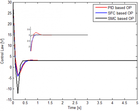
It can be seen from Figure 7 that the responses of the control signals for the three controllers are smooth and within the acceptable voltage range of the DC motor. Besides, it can be noticed that the chattering problem in the SMC is eliminated by the proposed reaching law. Moreover, Figure 8 shows the response of the three controlled systems for a unit step input. The performance evaluation is based on settling time, steady state error, maximum overshoot, and ITAE. The dynamics performance of the three controllers is reported in Table 4.
Figure 7. Control signals of the proposed controllers
Based on Figure 8 and Table 4, it can be revealed that the three controllers tuned by GTO are capable to control the system successfully with zero error steady state. However, the SMC has better dynamics performance than that of the other controller, in terms of reducing the settling time, overshoot, and ITAE index. For example, based on the results in Table 4, it can be seen that the settling time is reduced from 0.31 sec in the case of the PID controller and 0.35 sec in the case of the SF controller to 0.25 sec in the case of SMC. Furthermore, the SMC eliminates the overshoot in comparison to PID and SF controllers. The ITAE is reduced from 4.162 in the case of the PID controller and 3.81 sec in the case of SF controller to 2.573 sec in the case of SMC.
Figure 8. Response of the system using the proposed controllers
Table 4. Dynamic performances of the system using the proposed controllers without disturbance
|
Controller |
Settling Time (s) |
Error Steady State (rad) |
Maximum Overshoot (%) |
ITAE |
|
PID |
0.31 |
0 |
3.4 |
4.162 |
|
SF |
0.35 |
0 |
0.36 |
3.81 |
|
SMC |
0.25 |
0 |
0 |
2.573 |
To ensure the robustness of the proposed controllers to cope with uncertainties, an external torque disturbance has been applied to each controller after 1.6 sec of the simulation. Figure 9 plots the response of the three controlled systems for unit step input with disturbance. The performance of the system with disturbance is evaluated based on settling time and maximum undershoot overshoot. The dynamics performance of the three controllers with disturbance is reported in Table 5.
Figure 9. Response of the system using the proposed controllers with disturbance
Based on Figure 9 and Table 5, it can be observed that the SMC has better recovery performance than that of the other controller under the disturbance environment, in terms of reducing the settling time and undershoot. For example, based on the results in Table 5, it can be seen that the settling time is reduced from 1 sec in the case of the PID controller and 0.56 sec in the case of SF controller to 0 sec in the case of SMC. Moreover, the maximum undershoot is reduced from 29 in the case of the PID controller and 23 in the case of SF controller to 3.3 in the case of SMC.
Table 5. Dynamic performances of the system using the proposed controllers with disturbance
|
Controller |
Settling Time(s) |
Maximum Undershoot |
|
PID Controller |
1 |
29 |
|
SF Controller |
0.56 |
23 |
|
SMC |
0 |
3.3 |
From the aforementioned results, it can be concluded that SMC outperforms PID and SF controllers to control the angular position of the nonlinear propeller pendulum system.
The propeller pendulum system is a variant of the classical simple pendulum where a propeller motor is coupled at the end of the pendulum. The torque generated by the motor drives the pendulum to lift up and down. In this paper, three control structures, PID controller, SF controller and SMC, are proposed to make the angular position of the propeller pendulum follows the desired angular position. To ensure the best performance of each controller, GTO is employed to tune the design parameters of the controllers. Simulation results based on the n MATLAB environment show how’s that the three controllers tuned by GTO are capable to control the system successfully with zero error steady state. However, the result shows that the SMC exhibits a better response compared to PID and SF strategies in reducing the settling time, overshoot, and ITAE. Moreover, SMC-based GTO demonstrates considerable superiority to compensate for the effect of external disturbance.
|
ABSC |
Adaptive Backstepping Control |
|
ASTSMC |
Adaptive Super-Twisting SMC |
|
GA |
Genetic Algorithm |
|
GTO |
Gorilla Troops Optimization |
|
ITAE |
Integral Time of Absolute Error |
|
LQR |
Linear Quadratic Regulator |
|
PID |
Proportional-Integral-Derivative |
|
PSO |
Particle Swarm Optimization |
|
QDMC |
Quadratic Dynamic Matrix Control |
|
SF |
State Feedback |
|
SMC |
Sliding Mode Controller |
|
$a_{s m c}$ |
Tuning parameters>0 |
|
C |
Viscous damping coefficient |
|
d |
Distance from suspending point to mass center |
|
$e(t)$ |
Error between the measured output $x_1(t)$ and the desired output $x_d(t)$ |
|
$\dot{\mathrm{e}}(\mathrm{t})$ |
First derivative of $e(t)$ |
|
g |
Acceleration of gravity |
|
$g_n$ |
Coefficients |
|
$\mathrm{G}_{\text {sliverback }}$ |
Best solution |
|
GR(itr) |
Solution selected randomly |
|
GX(itr) |
Current solution |
|
GX(itr+1) |
New solution |
|
i |
Index for population |
|
itr |
Index for iteration |
|
J |
Moment of inertia |
|
$\mathrm{k}_1, \mathrm{k}_2, \mathrm{k}_3, \mathrm{k}_4, \mathrm{k}_7, \mathrm{k}_8, \mathrm{k}_9$ |
Coefficients |
|
$\mathrm{k}_5$ |
Random number between [-1, 1] |
|
$\mathrm{k}_6$ |
Random number between $\left[-\mathrm{k}_1, \mathrm{k}_1\right]$ |
|
$\mathrm{k}_d$ |
Derivative gain |
|
$\mathrm{k}_i$ |
Integral gain |
|
$\mathrm{k}_m$ |
Constant of the DC motor |
|
$\mathrm{k}_p$ |
Proportional gain |
|
$\mathrm{k}_{\mathrm{smc}}$ |
Adjusted parameter $>0$ |
|
$\mathrm{K}_{\mathrm{x}_1}, \mathrm{~K}_{\mathrm{x}_2}$ |
Feedback-weighted gains |
|
$\mathrm{K}_{\mathrm{x}_{\mathrm{d}}}$ |
Forward-weighted gain |
|
M |
Mass of propeller |
|
N |
Population size |
|
$\mathrm{p}_1, \mathrm{p}_2, \mathrm{p}_3$ |
Coefficients determined by the user between [0,1] |
|
$\mathrm{r}_1, \mathrm{r}_2, \mathrm{r}_3, \mathrm{r}_4, \mathrm{r}_5$ |
Random number between [0,1] |
|
$\mathrm{rn}_1$ |
Random number between $[0,N]$ |
|
$\mathrm{rn}_2$ |
Random number |
|
$s(t)$ |
Sliding surface |
|
$\dot{s}(t)$ |
First derivative of $s(t)$ |
|
sgn |
Sign function |
|
t |
Time |
|
$\mathrm{t}_{\text {sim }}$ |
Total simulation time |
|
$\mathrm{T}_{\mathrm{m}}$ |
Torque generated by the motor |
|
$\mathrm{T}_{\max }$ |
Maximum iteration |
|
$\mathrm{u}(\mathrm{t})$ |
Control law |
|
$x_1(t)$ |
Angle position |
|
$\dot{x}_1(t)$ |
First derivative of $x_1(t)$ |
|
$x_2(t)$ |
Angle velocity |
|
$\dot{x}_2(t)$ |
First derivative of $x_2(t)$ |
|
$x_d(t)$ |
Desired output |
|
$\dot{x}_d(t)$ |
First derivative of $\mathrm{x}_{\mathrm{d}}(\mathrm{t})$ |
|
$\ddot{x}_d(t)$ |
Second Derivative of $\mathrm{x}_{\mathrm{d}}(\mathrm{t})$ |
|
$\Gamma$ |
Adjusted parameter between [0,1] |
|
$\theta(\mathrm{t})$ |
Angle position |
|
$\dot{\theta}(\mathrm{t})$ |
Angle velocity |
|
$\ddot{\theta}(\mathrm{t})$ |
Angle acceleration |
[1] Taskin, Y. (2017). Fuzzy PID controller for propeller pendulum. Istanbul University - Journal of Electrical and Electronics Engineering (IU-JEEE), 17(1): 3175-3180.
[2] Mohammadbagheri, A., Yaghoobi, M. (2011). A new approach to control a driven pendulum with the PID method. In 13th International Conference on Modelling and Simulation, Cambridge, UK, pp. 207-211. https://doi.org/10.1109/UKSIM.2011.47
[3] Hamoudi, A.K., Rasheed, L.T. (2023). Design and implementation of adaptive backstepping control for position control of propeller-driven pendulum system. Journal Européen des Systèmes Automatisés, 56(2): 281-289. https://doi.org/10.18280/jesa.560213
[4] Al-Qassar, A.A., Al-Dujaili, A.Q., Hasan, A.F., Humaidi, A.J., Ibraheem, I.K., Azar, A.T. (2021). Stabilization of single-axis propeller-powered system for aircraft applications based on optimal adaptive control design. Journal of Engineering Science and Technology (JESTEC), 16(3): 1851-1869.
[5] Günel, O., Ankarah, A. (2017). Tuning PID controller using genetic algorithm and particle swarm optimization algorithm for single propeller pendulum. In 3rd Conference on Advances in Mechanical Engineering Istanbul 2017, 19-21 December 2017, Istanbul, Turkey,
[6] Farmanbordar, A., Zaeri, N., Rahimi, S. (2011). Stabilizing a driven pendulum using DLQR control. In 2011 Fifth Asia Modelling Symposium, Manila, Philippines, pp. 123-126. https://doi.org/10.1109/AMS.2011.32
[7] Raju, S.S., Darshan, T.S., Nagendra, B. (2012). Design of quadratic dynamic matrix control for driven pendulum system. International Journal of Electronics and Communication Engineering, 5(3): 363-370.
[8] Kizmaz, H., Aksoy, S., Mühürcü, A. (2010). Sliding mode control of suspended pendulum. 2010 Modern Electric Power Systems, Wroclaw, Poland, pp. 1-6.
[9] Al-Khazraji, H., Khlilb, S., Alabacy, Z. (2022). Solving mixed-model assembly lines using a hybrid of ant colony optimization and greedy algorithm. Engineering and Technology Journal, 40(1): 172-180. http://doi.org/10.30684/etj.v40i1.2153
[10] Al-Khazraji, H., Cole, C., Guo, W. (2018). Analysing the impact of different classical controller strategies on the dynamics performance of production-inventory systems using state space approach. Journal of Modelling in Management, 13(1): 211-235. https://doi.org/10.1108/JM2-08-2016-0071
[11] Mahmood, Z.N., Al-Khazraji, H., Mahdi, S.M. (2023). April. PID-based enhanced flower pollination algorithm controller for drilling process in a composite material. Annales de Chimie Science des Matériaux, 47(2): 91-96. https://doi.org/10.18280/acsm.470205
[12] Nagaraj, B., Murugananth, N. (2010). A comparative study of PID controller tuning using GA, EP, PSO, and ACO. In 2010 International Conference on Communication Control and Computing Technologies, Nagercoil, India, pp. 305-313. https://doi.org/10.1109/ICCCCT.2010.5670571
[13] Al-Khazraji, H., Rasheed, L.T. (2021). Performance evaluation of pole placement and linear quadratic regulator strategies designed for mass-spring-damper system based on simulated annealing and ant colony optimization. Journal of Engineering, 27(11): 15-31. https://doi.org/10.31026/j.eng.2021.11.02
[14] Mpanza, L.J., Pedro, J.O. (2020). Sliding mode control of an electromechanical actuator swashplate using cuckoo search optimisation algorithm. In 2020 3rd International Conference on Control and Robots (ICCR), Tokyo, Japan, pp. 204-210. https://doi.org/10.1109/ICCR51572.2020.9344335
[15] Singh, K., Nema, S., Padhy, P.K. (2014). Modified PSO-based PID sliding mode control for inverted pendulum. In 2014 International Conference on Control, Instrumentation, Communication and Computational Technologies (ICCICCT), Kanyakumari, India, pp. 722-727. https://doi.org/10.1109/ICCICCT.2014.6993054
[16] Furat, M., İlyas, E.K.E.R. (2012). Experimental evaluation of sliding-mode control techniques. Çukurova Üniversitesi Mühendislik-Mimarlık Fakültesi Dergisi, 27(1): 23-37.
[17] Rasheed, L.T., Yousif, N.Q., Al-Wais, S. (2023). Performance of the optimal nonlinear PID controller for position control of antenna azimuth position system. Mathematical Modelling of Engineering Problems, 10(1): 366-375. http://doi.org/10.18280/mmep.100143
[18] Al-Khazraji, H., Nasser, A.R., Khlil, S. (2022). An intelligent demand forecasting model using a hybrid of metaheuristic optimization and deep learning algorithm for predicting concrete block production. IAES International Journal of Artificial Intelligence, 11(2): 649. http://doi.org/10.11591/ijai.v11.i2.pp649-657
[19] Al-Khazraji, H., Khlil, S., Alabacy, Z. (2021). Cuckoo search optimization for solving product mix problem. Materials Science and Engineering, 1105(1): 012016. http://doi.org/10.1088/1757-899X/1105/1/012016
[20] Abdollahzadeh, B., Soleimanian Gharehchopogh, F., Mirjalili, S. (2021). Artificial gorilla troops optimizer: A new nature-inspired metaheuristic algorithm for global optimization. problems. International Journal of Intelligent Systems, 36(10): 5887-5958. https://doi.org/10.1002/int.22535
[21] Yamagiwa, J., Kahekwa, J., Basabose, A.K. (2003). Intra-specific variation in social organization of gorillas: Implications for their social evolution. Primates, 44: 359-369.
[22] Ghith, E.S., Tolba, F.A.A. (2023). Tuning PID controllers based on hybrid arithmetic optimization algorithm and artificial gorilla troop optimization for micro-robotics systems. IEEE Access, 11: 27138-27154. https://doi.org/10.1109/ACCESS.2023.3258187
[23] Al-Khazraji, H. (2022). Optimal design of a proportional-derivative state feedback controller based on meta-heuristic optimization for a quarter car suspension system. Mathematical Modelling of Engineering Problems, 9(2): 437-442. https://doi.org/10.18280/mmep.090219