Rafik Euldji | Redha Rebhi![]() | Mohammed Ayad Alkhafaji
| Mohammed Ayad Alkhafaji![]() | Omolayo M. Ikumapayi
| Omolayo M. Ikumapayi![]() | Esther T. Akinlabi
| Esther T. Akinlabi![]() | Stephen A. Akinlabi
| Stephen A. Akinlabi![]() | Karrar S. Mohsen | Younes Menni*
| Karrar S. Mohsen | Younes Menni*![]()
© 2023 IIETA. This article is published by IIETA and is licensed under the CC BY 4.0 license (http://creativecommons.org/licenses/by/4.0/).
OPEN ACCESS
This study aims to address the challenge of low-cost hardware implementation of a combined backstepping with fractional order PID (FOPID) controller for mobile robots in real-time applications. Moreover, this work proposes a self-designed mobile robot prototype that is easy to realize, low in cost, spares time, and reduces human effort. This robot platform was equipped with two DC motors with quadratic encoders and two passive wheels, controlled by an Arduino mega, where the software code was developed in the Matlab-Simulink environment, using Simulink support package for Arduino. Four case studies were conducted to demonstrate the effectiveness of the suggested methodology. Experimental results demonstrate improved trajectory tracking performance with less tracking error and smooth control efforts, and is capable of handling trajectories with continuous and non-continuous gradients.
intelligent robust controller, complex environment, Arduino mega, serial communication protocol, experimental study
Currently, the developments in science and technology enable the appearance of commercial robots in the industrial field, where the requirement for a programmable vehicle that can move in three-dimensional workspace for tasks execution is getting increasing every day. Wheeled mobile robots have become increasingly important in a range of industrial applications [1-6]. In order to achieve such challenging demands, a high efficiency control methodology with fast time response for tracking both speed and orientation angle during the task’s execution is required, while mobile robot interactions and their nonlinear structure make it challenging to implement control algorithms.
The problem of tracking trajectory is still fascinating and interests many investigators. Since the rapid progress of many indoor and outdoor applications that act in complex environment [7-23]. In addition, the majority of WMRs can be categorized as nonholonomic mechanical systems (pure rolling without side slipping motion). The motion of a WMR in this scenario carries three degrees of freedom, but under the nonholonomic restriction, it can only be controlled by two control inputs. These control issues have freshly interested a great attention of many researchers [7-23]. Each mechanism has its own specific dynamics propriety that it is different from one robot to another, which means a standard regulation technique is not available. For this purpose, realization of new and more precise control techniques that respond to task complexity is required.
In experience, reaching an acceptable path tracking performance for a WMR is a challenging task due to rapid changing of the process in real-time, the influence of the nonlinear dynamic, uncertainties, payload changes and external perturbation. In order to deal with disgust issues, a robust control method is required. Various powerful control approaches have been implemented practically to handle this problem, such as sliding mode control [11, 12], adaptive control [13-15], H-infinity control [16, 17], neural network control [18-20], fuzzy logic type-2 in the study [21, 22], and using the adaptive neuro-fuzzy inference (ANFIS) [23].
However, the old PID strategy still has been utilized in many industrial applications [24]. The reason behind this high popularity belongs to the facility of design and hardware implementation, with an acceptable performance obtained from this controller [24]. The appearance of the FOPID controller made a remarkable attention from many investigators, due to its over performance compared to the traditional PID controller [25-30]. In comparison to the integer-order PID controller, which has just three parameters to be tuned, five parameters, namely Kp, Ki, Kd, λ, and µ, can give better designed controllers, in terms of faster in time response and less overshoot [25, 30]. Tuning the FOPID parameter was challenging, in our previous study [31], a powerful meta-heuristic algorithm was proposed to solve the problem, where a comparative analysis was carried out using Matlab/Simulink environment to highlight the significant improvement of the chosen algorithm; this research intends to experimentally validate the previously described method.
The hardware realization of any fractional order system requires an expertise in the fractional calculus domain, which leads to a lot of investment in time. In addition, the fractional systems need a high-level of approximation approaches to represent the infinite memory of the process, therefore the discretization of any system should be determined carefully [26, 32, 33]. This makes it hardware implementation in real time a critical issue. Moreover, many research papers focused their investigation on solving this problem only for a specific application [33]. Most of these algorithms are tested in a MATLAB-Simulink environment, where the hardware implementation has been reached using on a rapid and powerful DSP processors [34-39]. This solution is hard to apply in the industry due to the big calculations demands and very costly too [40]. So, in order to get around the issue of high costs, some researchers used field-programmable gate arrays (FPGAs) [33, 40], which have evolved into an alternative option for achieving flexibility and higher accuracy but are still challenging to implement due to the complexity of the board [41], using the Programmable Logic Controllers (PLC) implementation, which is more suitable for industrial applications due to its simplicity and lower cost [41, 42]. Another approach that is more straightforward than FPGA implementations is one that is focused on ARM processors [43]. However, the demands for a standard, simple and also a low-cost hardware realization that can be applied in various projects is required. The appearance of the FOMCON toolbox [44], and simulink support package for Arduino seems to be promoting, since it has been utilized from many researchers in various field [45-49]; this makes us the inspiration for this contribution.
The objective of this study is to develop a low-cost hardware implementation of a trajectory tracking controller for wheeled mobile robots, capable of handling complex environments and executing various pre-defined trajectories with minimal tracking error. The proposed approach combines a fractional order PID (FOPID) controller with the Backstepping technique, and is designed to provide fast time response and robust control in the face of nonlinear dynamics, uncertainties, payload changes, and external perturbations.
The experimental setup consists of a self-designed wheeled mobile robot platform, equipped with two DC motors with quadratic encoders and two passive wheels, controlled by an Arduino mega. The software design involves developing hardware code in the Matlab-Simulink environment, using the Simulink support package for Arduino. Experimental results will be presented to demonstrate the effectiveness of the proposed approach in trajectory tracking mobile robot platform has been constructed to examine the overall performance of the proposed methodology in real-time. The architecture of the WMR based on the deferential drive mechanism consists of two DC motor with quadratic encoders and two passive wheels, an Arduino mega to read the sensory data. The Arduino acts as a slave microcontroller, connected with a master PC, communicate with each other based on a serial communication protocol. Four case studies are offered to confirm the validity of the proposed controllers.
The activities are divided into three parts, consisting of hardware design, software design, and experimental results. The hardware part includes the mechanical and electrical design of the robot platform, where the software part is focusing on developing the hardware code in the Matlab-Simulink environment, using the Simulink support package for Arduino.
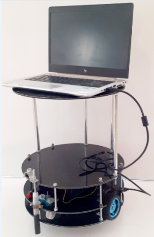
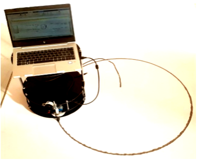
Figure 1 depicts the self-built mobile robot platform. It consists of a base carrying a laptop, power supply, the electronic circuit and a white board marker, in order to act as a 2D printer, where Figure 2 shows a simplified architecture of the complete control strategies of the system. Focusing on the block diagram:
Figure 1. Self-designed robot plat form
Figure 2. The proposed control architecture
At first a Simulink support package need to be installed, to upload directly the Simulink program to the controller board (Arduino mega) without any programming (details are in software description). Simulink and the Arduino Mega microcontroller are connected via USB serial communication (57000 baud rate, 8 bits). Using the signal input from the MATLAB environment, Arduino makes a judgment before generating PWM signals to control the right and left wheels, where a L298n driver amplify the control action to 12V, to control the dc motors, supplied by a 6V battery where a boost converter amplify the voltage to 12V, the quadrature encoders extract the information from the environment and send back the data to PC, the linear speed and the orientation are estimated using the forward kinematics of the mobile robot.
(a)
(b)
(c)
(d)
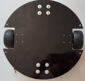
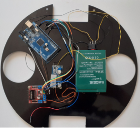
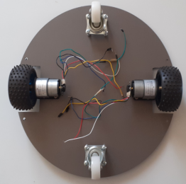
Figure 3. Design of the mechanical platform: (a) Top view of the base, (b) the electronic circuit location in the base, (c) Bottom view, (d) the assembled platform
The differential drive system is one of the more affordable options for navigating mobile robots. One of the most straightforward driving systems for a mobile robot, it is primarily meant for indoor navigation. There are two parts in this section.
3.1 The self designed robot platform
The differential drive robot has two wheels positioned on a single axis, each of which is driven by a distinct motor. Caster wheels are the two supporting wheels. This guarantees the robot's stability and weight distribution. Figure 3 depicts the differential drive system's self-designed platform, and Table 1 lists the platform's hardware components.
Table 1. Component of the platform’s hardware
|
Size platform |
The platform has a circular floor plan with a diameter of 34 cm |
|
Wheels |
Radius of wheel, R=0.04 m |
|
Drive type |
Differential drive with two caster wheels |
|
Maximum speed |
0.3m/s |
|
Motor type |
DC motors 12V, 107 RPM, with gear ratio 1:90 and stall tork 20kg.cm at maximum current is 3.4A |
|
Encoder resolution |
Hall * Ratio=11*90=990 PPR (pulse per revolution) |
|
Controller |
Arduino Mega 2560 board |
|
Power |
6V, 4Ah battery with boost converter |
|
Weight |
4kg |
|
Payload |
5kg |
3.2 The electronics circuit design
The power supply is taken from a (6V) battery with a maximum current up to 4Ah, where a boost converter is used to convert the voltage from 6V to 12V. In order to provide energy to both DC motors and also the power electronic circuits, which is a L298n driver (see Figure 4). This H-bridge driver uses its own regulator to lower the voltage to 5V in order to power the ARDUINO mega controller board. The ground connection of the battery is common to the entire system electronics of the robot. The power control circuit of the motors (L298n) contains two full H-bridges of with maximum supporting current up to 2A. Although motors may require more current (up to 3A for a single motor). The added heat sink in the module allows it to work without heating for this application. Moreover, this circuit can be purchased at a very low cost which make it ideal for our application.
Figure 4. Wiring diagram of the entire hardware
To power the Arduino board, the driver's 5V pin is connected to the Arduino's Vin pin. In order to control the direction of motor 1, the L298n driver's input 1 and input 2 pins are linked to the Arduino's pins 07 and 08, respectively. Motor 2 is controlled by the L298n driver's input 3 and input 4 pins, which are connected to the Arduino's pins 11 and 10, respectively. In order to use PWM signals to regulate the speed of motors, Enable A and Enable B are connected to Arduino's pins 9 and 12, respectively.
The encoders of the DC motors are magnetic type, with two digital outputs (A and B) of 5V pulses that connect to inputs of Arduino interrupt. They allow you to get a resolution of 990 counts per turn. The ARDUINO mega has six external interruption lines, where pins 18, 19, 20, and 21 are used for signals A and B of the encoders of the two actuators.
The MATLAB/Simulink environment and the Arduino board were combined using the Simulink Support Package for Arduino Hardware. The decision was made based on the many benefits that this toolbox provides, including the ability to build and execute Simulink models in numerical fields and to provide a block library for configuring and interacting with Arduino sensors, actuators, and communication interfaces using USB cables. With this method, you may create control algorithms in Simulink and upload them without any code to the hardware platform (Arduino board) [45]. These toolboxes are in charge of making data communication between the computer and the robot and vice versa possible. This tool, which can be easily discovered in MATLAB's home tab's add-on section, automatically generates C and C++ code for embedded systems. Figure 5 shows a window displaying the Arduino blocks library.
The package makes it possible to carry out operations like [45, 46]:
- Get data from analog and digital sensors from the Arduino board;
- Control devices that have PWM and digital outputs;
- Utilize a USB cable to communicate with an Arduino board; and
- Use the SPI (Serial Peripheral Interface) or the IIC (Inter Integrated Circuit) (I2C) to access peripheral devices and sensors.
External Mode and Normal Mode are the two primary means of communication between the board and the PC. Both approaches offer advantages and disadvantages, but depending on the project, one approach can turn out to be more advantageous than the other [50].
Simulink IO's normal mode:
You can use Simulink I/O to establish a connection to external hardware, like an Arduino, and download applications to it. Although it is a quick way to run your code and interact with the I/O peripherals, the main drawback of this connection method is that data recording is more challenging than with external mode.
External mode:
By using the external mode, you can adjust parameters and track data in real-time, which eliminates the need to recompile or download the model each time a change is made. When external mode is activated, the Arduino and computer communicate over the serial port. Therefore, the USB must be linked between them in order for it to operate in external mode. The appeal of using external mode for these tests lies in its capacity to adjust and track changes in real-time. Being able to observe the immediate results of your modifications on the hardware has advantages for you. This real-time changing capability comes at a price, though, since the serial port must be kept open and has a finite amount of bandwidth in order to communicate back and forth. The program's speed can be impacted by this restriction. Thus, compared to normal mode, this mode is slower [50].
It is important to note that a different option, Deploy to Hardware, allows us to export all of the code to the microcontroller without requiring a PC connection. However, in this instance, the external mode will be used because we'll be using Simulink's Scope blocks as oscilloscopes for the most crucial signals, such the control signal or the plant output.
Figure 5. Arduino blocs library
4.1 The complete simulink model
Figure 6 reports the complete bloc diagram of the designed simulink model which is responsible for controlling the robot platform, it consists of a trajectory generator programmed based on a Matlab function responsible for generating the reference signal, a backstepping controller is located in external loop programmed using a Matlab function too, responsible for the kinematic control actions. Two discrete FOPID controller blocs in the internal loop were created by benefiting from FOMCON toolbox (description will be in next sections), one for speed control and the other for orientation control. The output signals were sent to the two wheels using PWM technique, the quadrature encoder used to determine the robot localization.
4.2 FOPID controller implementation
In 1999, Podlubny [9, 10, 44] introduced the fractional proportional integral derivative (FOPID) which incorporates two new fractional components, λ and μ, into the traditional PID controller. These new components are a fractional integrator and differentiator, respectively, and are represented by the non-integer-order operator in Eq. (1):
$D_n^t=\left\{\begin{array}{c}\frac{d^n}{d t^n} &n>0 \\ 1 & n=0 \\ \int_t^a d t^n &n<0\end{array}\right.$ (1)
The process is bounded by the lower limit (t) and upper limit (a), and is operated upon by the constant integral differential operator $n \in \mathbb{R}$. There exist three primary definitions of fractional calculus, namely Riemann Liouville (RL), GrünwaldL and nikov (GL), and Caputo. Among these, the Caputo method is the most widely used definition in engineering applications, and is represented by Eq. (2).
$D_n^t f(t)= \frac{1}{\Gamma(\alpha-\mathrm{n})} \int_a^t \frac{f^n(\tau)}{(t-\tau)^{n-\alpha+1}} \quad d \tau \,\,for\,\, n-1 \leq n \leq \alpha$ (2)
Although the term (sα) lacks an analytical solution, it possesses a fractional order that is difficult to implement. As a result, numerical solutions like the Oustaloup approximation are commonly used [9, 10, 44].
$s^\alpha \approx K \prod_{n=-N}^N \frac{1+\frac{s}{\omega_{z, n}}}{1+\frac{s}{\omega_{p, n}}} \alpha>0$ (3)
The variable N represents the quantity of poles/zeros.
Figure 6. The complete designed simulink bloc diagram
Figure 7. Block diagram of fractional order
The block diagram in Figure 7 depicts the parallel structure of the FOPID controller, where the input is E(S) and the output is U(S). Eq. (4) provides the time domain expression of the transfer function for the Fractional Order PID (FOPID), while Eq. (5) gives its Laplace domain representation:
$u(t)=K_p e(t)+k_i D_t^{-\lambda} e(t)+K_d D_t^\mu e(t)$ (4)
$C(s)=\frac{U(s)}{E(s)}=K_p+\frac{K_i}{S^\lambda}+K_d S^\mu$ (5)
The constants Kp, Ki, and Kd are the proportional, integral, and derivative gain values, respectively. The fractional orders of the integral and derivative terms are denoted by λ and μ.
The FOMCON toolbox was selected for the FOPID implementation [44]. A series of graphical user interfaces intended to make the toolbox easier to use. The aim to find a comprehensive solution for effective controller design and analog/digital implementation is another driving force behind the development of FOMCON. This last one provides a collection of tools specifically for using fractional-order PID controllers.
4.3 Speed control
The PWM ratio can be changed to regulate the speed of a DC motor. By changing the duty cycle of pulses while maintaining a constant carrier signal frequency (period) and pulse amplitude, PWM is a technique for modulating a signal. The computer controls peripherals via digital output pins operating in PWM mode.
However, due to the limited current and constant output voltage, the embedded computer is unable to connect to a DC motor directly. As a result, the L298N motor driver is used by the embedded computer to power the motor. The two motors are driven by the motor driver once it receives an on/off signal from the Arduino mega.
A DC motor driver can turn a DC motor on or off, but does not have the ability to control speed. Pulse Width Modulation (PWM) is used by the embedded computer to quickly turn on and off these switches while also controlling the direction and speed of the motor.
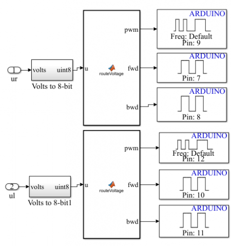
Figure 8 shows the designed simulink model that generates the PWM signals. The frequency of the waveform is constant at approximately 490 Hz. The Output of the first FOPID controllers (see Figure 6) is responsible for controlling the right wheel velocity by sending the control signal to Arduino digital pin 09 which is the PWM pulse width modulation pin. The duty cycle is controlled from 0 to 255. If logic 0 then duty cycle is zero means the speed of machine is 0 RPM. While logic 255 then speed of motor is 107 RPM that means maximum mobile robot speed, here a Matlab function has been created (see Figure 8) to deal with the PWM output signal and controlling the direction of the right wheel at the same time, using PIN 09, PIN 07 and PIN 08, the Matlab function here is to make sure that the L298n driver will not short circuit. The same technique has been applied for controlling the left wheel using the second FOPID controller, using pin 12 for PWM signal were, pin 10 and pin 11 for the direction of left wheel.
4.4 Motor speed calculation from encoder
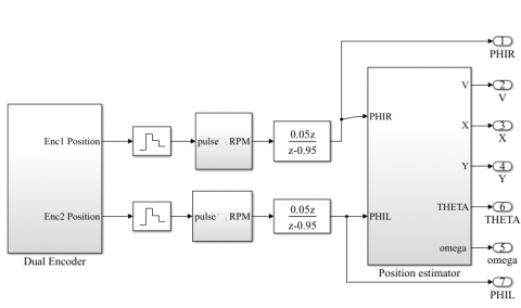
The quadrature encoder, a sensor that produces data in the form of a square wave, enables control of the movement of the vehicle's wheels. The motor speed and the number of pulses are connected. Figures 9 (a) and (b) illustrates the Simulink model of the pulse count and its conversion to RPM utilizing pins 18, 19, 20, and 21 for both DC motors and a "Rollover block adjustment".
Figure 8. The designed simulink model for the PWM signals and orientation
This bloc was produced because to the fact that the buffer used to keep track of the number of counts can only handle values between -32768 and 32767; it needs 16 bits, 15 of which are used for the number and 1 for the sign.
In order to establish whether a rollover has occurred, this subsystem compares the current number of counts to the number of counts from the previous sample (at 32767 or at -32768). If a rollover has occurred, the rollover is then removed from the accumulated number of counts.
The sampling time is: 0.005 seconds. In this study, the encoder of geared DC motor has a reduction ratio of 1:90 (metal gearbox) providing a resolution of 11 pulse per revolution. So, the counts per revolution (PPR) of the motor speed and gear ratio can then be calculated: PPR=11*90=990. The Gain block used for converting pulse to RPM is shown in Figure 9(a). Since the output signal has quite a lot of noise. A transfer function filter block was then applied here to reduce some noise to a certain extent.
(a)
(b)
Figure 9. The designed simulink model for encoder reading: (a) the structure of the RPM reading, and (b) the S function bloc and the rollover bloc
4.5 Pose estimation
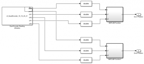
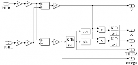
Figure 10. The designed simulink model for pose estimation
The 'Dead Reckoning' or 'Odometric Localization’ procedure uses information from the quadrature encoders in the right and left wheels to estimate a robot's coordinates. The robot's location, linear velocity, and angle of orientation are then predicted using the forward kinematics model. The robot pose is then estimated by integrating the data across time beginning at a specified initial point (x(0) and y(0)). The Simulink model that corresponds to the estimation methodology is shown in Figure 10.
The above simulink bloc was realised using the following kinematic model from our previous contribution [9, 10].
$\left[\begin{array}{c}\dot{x}_a \\ \dot{y}_a \\ \dot{\theta} \\ \dot{\varphi}_R \\ \dot{\varphi}_L\end{array}\right]=\left[\begin{array}{cc}\cos \theta & 0 \\ \sin \theta & 0 \\ 0 & 1 \\ \frac{1}{R} & \frac{-L}{R} \\ \frac{1}{R} & \frac{-L}{R}\end{array}\right]\left[\begin{array}{l}v \\ \omega\end{array}\right]=\frac{1}{2}\left[\begin{array}{cc}R \cos \theta & R \cos \theta \\ R \sin \theta & R \sin \theta \\ \frac{R}{L} & -\frac{R}{L} \\ 2 & 0 \\ 0 & 2\end{array}\right]\left[\begin{array}{c}\dot{\varphi}_R \\ \dot{\varphi}_L\end{array}\right]$ (6)
Although this method is the most fundamental one used in mobile robotics, it is frequently employed in industrial robotics applications that don’t need highly accurate location estimation or as a redundant backup system for verification and error control. The wheels’ alignment must be adjusted, and the diameters of the wheels must match [51]. Additionally, a workspace's floor contact should be flat and smooth to prevent slippage brought on by variations in the wheels’ points of contact. More detail can be found in the study [9, 10].
The constructed mobile robot platform mentioned in the preceding section was used in trials to track four different intended trajectories in order to demonstrate the resilience of the proposed control strategy.
The method put into practice illustrates how the system behaves in terms of vehicle orientation, velocity control, and tracking errors when the FOPID and the backstepping controller are combined. Furthermore, research looks into the capacity to follow any trajectories with both continuous and non-continuous gradients. In order to highlight the distinctions and similarities between employing various trajectories, these comparisons are carried out under identical circumstances.
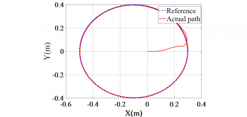
5.1 Case study (1): Tracking circular trajectory
First, a desired circular trajectory was used to confirm the applicability of the provided control mechanism to follow the continuous gradient with a constant rotation radius. Figure 11(a) shows a circular trajectory drawn on a white board using a platform that has been specifically developed, and Figure 11(b) shows estimated values in the XY coordinate.
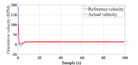
The motion of this trajectory is a continuous gradient trajectory. As a result, the first fractional order PID controller receives the difference in error between the desired and actual linear velocity. Figure 11(a) depicts the results of the speed control action, which track and converge to the intended reference velocity. The reference and actual orientation outputs of the second FOPID controller are shown in Figure 12(b). The orientation errors are kept close to zero, as can be shown.
(a)
(b)
Figure 11. Circular path: (a) the actual circle trajectory, (b) the estimated values from encoders
(a)
(b)
Figure 12. Circular path control efforts: (a) the tracked speed, (b) the tracked orientation
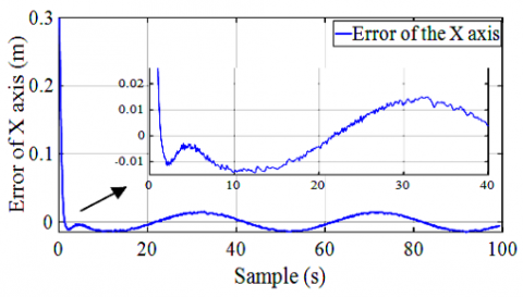
Figures 13 (a), (b), (c) and (d) show the errors according to the X, Y, theta and the error of distance. As represented in Y, from the previous response estimated from the encoders we can say that the control methodologies have been successfully realized for the circular trajectory.
(a)
(b)
(c)
(d)
Figure 13. The tracking errors of the circular path: (a) error of X axis, (b) error of Y axis, (c) error of the orientation, (d) error of the distance
5.2 Case study (2): Tracking lemniscates trajectory
Other continuous gradient routes include the lemniscate trajectory. Despite having a nearly identical orientation to a circular trajectory, a lemniscate trajectory is a planar curve with the distinctive shape of two loops that come together in the middle (central point). Because it is traveling while changing coordinate directions, it exhibits a roundabout motion. The equations from our earlier contributions [9, 10, 31] are used to generated the lemniscate trajectory. Figure 14(a) shows a 2D print of the infinity trajectory of the actual robot platform, and Figure 14(b) shows estimated data from quadrature encoders of the desired and actual lemniscate trajectories. Based on the employment of the FOPID controllers and the back-stepping controller in combination, it exhibits extremely good response and reasonable trajectory tracking performance.
(a)
(b)
Figure 14. (a) The 2D print of the infinity trajectory, (b) estimated XY plane for infinity path
(a)
(b)
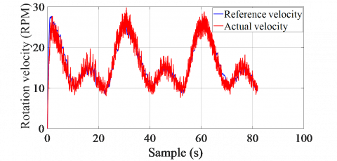
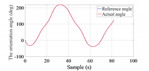
Figure 15. Lemniscate control efforts: (a) the tracked speed, (b) the tracked orientation
Figure 15(a) displays the estimated control actions from the encoders that demonstrate the efforts required from the robot vehicle to track the velocity. The data action is changed from a linear velocity (m/sec) to a rotation speed in this case (revolution per minute: RPM). Figure 15(b) displays the output efforts for the orientation angle control. The figures demonstrate a system actuator's realistic response to such a trajectory.
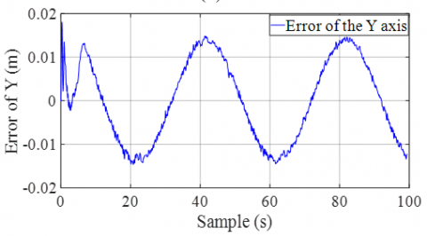
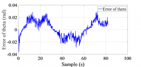
The errors according to the X, Y, theta orientation, and distance error are shown in Figures 16 (a), (b), (c) and (d), respectively. From the previous response estimated from the encoders and the real 2D print of the trajectory, we can say that the control methodologies have been successfully realized.
(a)
(b)
(c)
(d)
Figure 16. Tracking errors of lemniscates: (a) error of X-axis (b) error of Y-axis, (c) error of the orientation, and (d) error of the distance
5.3 Case study (3): Tracking quadrifolium trajectory
The trajectory of the quadrifolium is categorized as a continuous gradient path. Although a quadrifolium trajectory has a nearly identical orientation to a lemniscate’s trajectory, it is a planar curve with a distinctive form that consists of four loops that come together in the middle.
This path has been executed using the following equations [10]:
$x_R(n)=0.5 * \sin ^2\left(2 * \pi * \frac{t}{30}\right) * \cos \left(2 * \pi * \frac{t}{30}\right)$ (7)
$y_R(n)=0.5 * \cos ^2\left(2 * \pi * \frac{t}{30}\right) * \sin \left(2 * \pi * \frac{t}{30}\right)$ (8)
It is far more difficult to realize than lemniscates. Figure 17(a) shows the 2D print of the quadrifolium trajectory made using the actual robot platform, and Figure 17(b) shows approximated data obtained from quadrature encoders of the planned and actual quadrifolium trajectories.
(a)
(b)
Figure 17. (a) The 2D print of the quadrifolium trajectory, (b) estimated XY plane for quadrifolium path
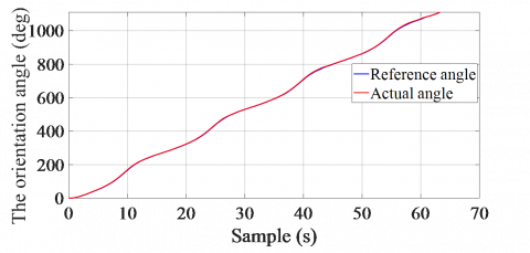
Figure 18(a) displays the predicted control actions from the encoders that illustrate the efforts required from the robot vehicle to track speed. Here, the data actions are translated from linear velocity (m/sec) to a rotation velocity (revolution per minute: RPM). Figure 18(b) shows the output attempts for the orientation angle control. The figures demonstrate a system actuator's realistic response to such a trajectory.
(a)
(b)
(c)
(d)
(e)
(f)
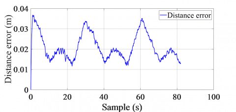
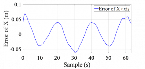
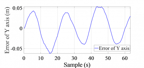
Figure 18. Quadrifolium path control efforts: (a) the tracked speed, (b) the tracked orientation, (c) error of X-axis, (d) error of Y-axis, (e) orientation error, and (f) distance error
The errors according to the X, Y, orientation angle, and distance errors are displayed in Figures 18 (c), (d), (e) and (f), respectively. From the previous response estimated from the encoders and the real 2D print of the trajectory, we can say that the control methodologies have been successfully realized with a low tracking error.
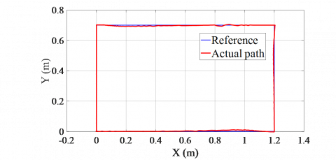
5.4 Case Study (4): Tracking rectangular trajectory
This study generates a non-continuous gradient trajectory, which results in an instantaneous change in the orientation at the connecting point while the WMR's path is being executed. A sharp, shaped trajectory is one that has several points of inflection, and the rectangular trajectory falls into this category. This example has been used to demonstrate the performance and capacity of the backstepping and FOPID controller when used together to handle situations like these.
(a)
(b)
Figure 19. (a) The 2D print of the rectangular path, (b) estimated XY plane for rectangular path
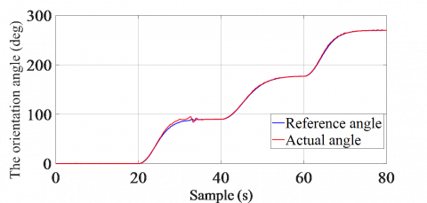
Figure 19(a) shows the 2D print of the square trajectory, and Figure 19(b) shows the estimated XY plane coordinates obtained from DC encoders of the desired and actual trajectories. The control actions estimated from the encoders which shows the efforts needed from the robot vehicle to track the speed is given in Figure 20(a). Here, the data action is converted from linear velocity (m/sec) to a rotation velocity (revolution per minute: RPM), the output efforts for the orientation angle control are given in Figure 20(b). The figures show a good response of system actuators for such a trajectory.
(a)
(b)
(c)
(d)
(e)
(f)
Figure 20. Control efforts of the rectangular trajectory: (a) the tracked speed, (b) the tracked orientation, (c) error of X-axis, (d) error of Y-axis, (d) angle error, and (e) distance error
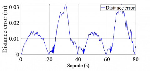
Figures 20 (c), (d), (e) and (f) shows the errors according to the X, Y coordinate, the theta orientation and the distance error respectively. Due to the quick changes in orientation at the corners of the rectangle, the control techniques have been successfully implemented with an acceptable tracking error, according to the prior response calculated from the encoders and the actual 2D print of the trajectory.
For a self-designed robot vehicle, a real-time implementation of a mixed fractional order PID controller and backstepping method has been developed. The device uses an encoder sensor to simultaneously locate itself and detect its surroundings. Based on the quadratic encoders, the WMR's travel distances and orientation have been estimated. To deal with the disturbance caused by DC motors, a noise filter has been introduced utilizing forward kinematics. In order to verify and validate the control technique, the platform based on the embedded system is explored utilizing four significant case studies. The first case study used a circular trajectory with a constant rotation radius and an intentionally continuous gradient. The third case study also used a smooth, quadrifolium-based trajectory, however it was more difficult to realize. The last trajectory is a rectangular one with a clearly non-continuous gradient. Experimental results show that the system works well and have confirmed the simulation results of our previous proposed technique. Moreover, the prototype is easy to realize, low in cost, spares time, and reduces human effort. Applying the proposed methodology in another mobile robot types seems to be motivating, such the unmanned Aerial vehicle. Consequently, it has been seen that some results can be ameliorated in the future especially for non-continuous trajectory. As perspectives we suggest to implement the adaptive Neuro- Fuzzy inference system (ANFIS), in real time application. The trajectory tracking and navigation problem can be going up to a new level and more robust using new embedded processors like the raspberry pi 4, and the FPGA, using vision sensors like the Kinect camera, an ultrasonic sensor like the HC-SR04 for the obstacle avoidance, and the Mems technology have a part too in developing the robot platform. A multi-agent architecture needs to be done in order to fix the problems that a single mobile robot can’t handle in complicate scenarios.
[1] Hercik, R., Byrtus, R., Jaros, R., Koziorek, J. (2022). Implementation of autonomous mobile robot in smartfactory. Applied Sciences, 12(17): 8912. https://doi.org/10.3390/app12178912
[2] Maher, N., Elsheikh, G.A., Ouda, A.N., Anis, W.R., Emara, T. (2022). Design and implementation of a wireless medical robot for communication within hazardous environments. Wireless Personal Communications, 122(2): 1391-1412. https://doi.org/10.1007/s11277-021-08954-7
[3] Holland, J., Kingston, L., McCarthy, C., Armstrong, E., O’Dwyer, P., Merz, F., McConnell, M. (2021). Service robots in the healthcare sector. Robotics, 10(1): 47. https://dx.doi.org/10.3390/ robotics10010047
[4] Saputra, R.P., Rakicevic, N., Kuder, I., Bilsdorfer, J., Gough, A., Dakin, A., Kormushev, P. (2021). ResQbot 2.0: An improved design of a mobile rescue robot with an inflatable neck securing device for safe casualty extraction. Applied Sciences, 11(12): 5414. https://doi.org/10.3390/app11125414
[5] Solanes, J.E., Muñoz, A., Gracia, L., Tornero, J. (2022). Virtual reality-based interface for advanced assisted mobile robot teleoperation. Applied Sciences, 12(12): 6071. https://doi.org/10.3390/app12126071
[6] Fue, K.G., Porter, W.M., Barnes, E.M., Rains, G.C. (2020). An extensive review of mobile agricultural robotics for field operations: Focus on cotton harvesting. AgriEngineering, 2(1): 150-174. https://doi.org/10.3390/agriengineering2010010
[7] Pliego-Jiménez, J., Martínez-Clark, R., Cruz-Hernández, C., Arellano-Delgado, A. (2021). Trajectory tracking of wheeled mobile robots using only Cartesian position measurements. Automatica, 133: 109756. https://doi.org/10.1016/j.automatica.2021.109756
[8] Nascimento, T.P., Dórea, C.E.T., Gonçalves, L.M.G. (2018). Nonlinear model predictive control for trajectory tracking of nonholonomic mobile robots: A modified approach. International Journal of Advanced Robotic Systems, 15(1): 1729881418760461. https://doi.org/10.1177/1729881418760461
[9] Euldji, R., Batel, N., Rebhi, R., Lorenzini, G., Jarasthitikulchai, N., Menni, Y., Sudsutad, W. (2022). Optimal design and performance comparison of a combined ANFIS-PID with back stepping technique, using various meta-heuristic algorithms to solve wheeled mobile robot trajectory tracking problem. Journal Européen des Systèmes Automatisés, 55(3): 281-298. https://doi.org/10.18280/jesa.550301
[10] Euldji, R., Batel, N., Rebhi, R., Skender, M.R. (2022). Optimal ANFIS-FOPID with back-stepping controller design for wheeled mobile robot control. Journal of Control Engineering and Applied Informatics, 24(2): 57-68.
[11] Goswami, N.K., Padhy, P.K. (2018). Sliding mode controller design for trajectory tracking of a non-holonomic mobile robot with disturbance. Computers & Electrical Engineering, 72: 307-323. https://doi.org/10.1016/j.compeleceng.2018.09.021
[12] Yang, Y., Yan, X., Sirlantzis, K., Howells, G. (2019). Application of sliding mode trajectory tracking control design for two-wheeled mobile robots. In 2019 NASA/ESA Conference on Adaptive Hardware and Systems (AHS), IEEE, pp. 109-114. https://doi.org/10.1109/AHS.2019.00012
[13] Cui, M., Liu, H., Liu, W., Qin, Y. (2018). An adaptive unscented kalman filter-based controller for simultaneous obstacle avoidance and tracking of wheeled mobile robots with unknown slipping parameters. Journal of Intelligent & Robotic Systems, 92(3): 489-504. https://doi.org/10.1007/s10846-017-0761-9
[14] Alakshendra, V., Chiddarwar, S.S. (2017). Adaptive robust control of Mecanum-wheeled mobile robot with uncertainties. Nonlinear Dynamics, 87(4): 2147-2169. https://doi.org/10.1007/s11071-016-3179-1
[15] Kang, Z., Zou, W., Ma, H., Zhu, Z. (2019). Adaptive trajectory tracking of wheeled mobile robots based on a fish-eye camera. International Journal of Control, Automation and Systems, 17(9): 2297-2309. https://doi.org/10.1007/s12555-019-0006-8
[16] Lafmejani, A.S., Farivarnejad, H., Berman, S. (2020). H∞-optimal tracking controller for three-wheeled omnidirectional mobile robots with uncertain dynamics. In 2020 IEEE/RSJ International Conference on Intelligent Robots and Systems (IROS), IEEE, pp. 7587-7594. https://doi.org/10.1109/IROS45743.2020.9341752
[17] Ahmad, N.S. (2020). Robust h∞-fuzzy logic control for enhanced tracking performance of a wheeled mobile robot in the presence of uncertain nonlinear perturbations. Sensors, 20(13): 3673. https://doi.org/10.3390/s20133673
[18] Bozek, P., Karavaev, Y.L., Ardentov, A.A., Yefremov, K.S. (2020). Neural network control of a wheeled mobile robot based on optimal trajectories. International Journal of Advanced Robotic Systems, 17(2): 1729881420916077. https://doi.org/10.1177/17298814209160
[19] Szeremeta, M., Szuster, M. (2022). Neural tracking control of a four-wheeled mobile robot with Mecanum Wheels. Applied Sciences, 12(11): 5322. https://doi.org/10.3390/app12115322
[20] Foroughi, F., Chen, Z., Wang, J. (2021). A CNN-based system for mobile robot navigation in indoor environments via visual localization with a small dataset. World Electric Vehicle Journal, 12(3): 134. https://doi.org/10.3390/wevj12030134
[21] Handayani, A.S., Alkausar, J., Husni, N.L. (2021). Implementation of fuzzy logic type-2 on mobile robot navigation system. In 4th Forum in Research, Science, and Technology (FIRST-T1-T2-2020), pp. 613-619.
[22] Al-Mallah, M., Ali, M., Al-Khawaldeh, M. (2022). Obstacles avoidance for mobile robot using type-2 fuzzy logic controller. Robotics, 11(6): 130. https://doi.org/10.3390/robotics11060130
[23] Gharajeh, M.S., Jond, H.B. (2022). An intelligent approach for autonomous mobile robots path planning based on adaptive neuro-fuzzy inference system. Ain Shams Engineering Journal, 13(1): 101491. https://doi.org/10.1016/j.asej.2021.05.005
[24] Borase, R.P., Maghade, D.K., Sondkar, S.Y., Pawar, S.N. (2021). A review of PID control, tuning methods and applications. International Journal of Dynamics and Control, 9(2): 818-827. https://doi.org/10.1007/s40435-020-00665-4
[25] Zhang, J., Jin, Z., Zhao, Y., Tang, Y., Liu, F., Lu, Y., Liu, P. (2020). Design and implementation of novel fractional-order controllers for stabilized platforms. IEEE Access, 8: 93133-93144, https://doi.org/10.1109/ACCESS.2020.2994105
[26] Abdelbaky, M.A., Emara, H.M., El-Hawwary, M.I., Bahgat, A., Liu, X. (2020). Implementation of fractional-order PID controller using industrial DCS with experimental validation. In 2020 IEEE 4th Conference on Energy Internet and Energy System Integration (EI2), Wuhan, China, pp. 4407-4413. https://doi.org/10.1109/EI250167.2020.9347159
[27] Ammar, H., Ibrahim, M., Azar, A., Shalaby, R. (2020). Gray wolf optimization of fractional order control of 3-omni wheels mobile robot: Experimental study. In 2020 16th International Computer Engineering Conference (ICENCO), Cairo, Egypt, pp. 147-152. https://doi.org/10.1109/ICENCO49778.2020.9357384
[28] Bernardes, N.D., Castro, F.A., Cuadros, M.A., Salarolli, P.F., Almeida, G.M., Munaro, C.J. (2019). Fuzzy logic in auto-tuning of fractional PID and backstepping tracking control of a differential mobile robot. Journal of Intelligent & Fuzzy Systems, 37(4): 4951-4964. https://doi.org/10.3233/JIFS-181431
[29] Barakat, M. (2022). Novel chaos game optimization tuned-fractional-order PID fractional-order PI controller for load-frequency control of interconnected power systems. Protection and Control of Modern Power Systems, 7(1): 1-20. https://doi.org/10.1186/s41601-022-00238-x
[30] Hsu, C.H., Cheng, S.J., Chang, T.J., Huang, Y.M., Fung, C.P., Chen, S.F. (2022). Low-cost and high-efficiency electromechanical integration for smart factories of IoT with CNN and FOPID controller design under the impact of COVID-19. Applied Sciences, 12(7): 3231. https://doi.org/10.3390/app12073231
[31] Euldji, R., Batel, N., Rebhi, R., Kaid, N., Tearnbucha, C., Sudsutad, W., Menni, Y. (2022). Optimal backstepping-FOPID controller design for wheeled mobile robot. Journal European des Systemes Automatises, 55: 97-107. https://doi.org/10.18280/jesa.550110
[32] Tepljakov, A., Petlenkov, E., Belikov, J. (2014). Embedded system implementation of digital fractional filter approximations for control applications. In 2014 Proceedings of the 21st International Conference Mixed Design of Integrated Circuits and Systems (MIXDES), Lublin, Poland, pp. 441-445. https://doi.org/10.1109/MIXDES.2014.6872237
[33] Tolba, M.F., Saleh, H., Mohammad, B., Al-Qutayri, M., Elwakil, A.S., Radwan, A.G. (2020). Enhanced FPGA realization of the fractional-order derivative and application to a variable-order chaotic system. Nonlinear Dynamics, 99(4): 3143-3154. https://doi.org/10.1007/s11071-019-05449-w
[34] Jiangbo, Z., Junzheng, W. (2017). The fractional order PI control for an energy saving electro-hydraulic system. Transactions of the Institute of Measurement and Control, 39(4): 505-519. https://doi.org/10.1177/0142331215610184
[35] Lino, P., Maione, G., Stasi, S., Padula, F., Visioli, A. (2017). Synthesis of fractional-order PI controllers and fractional-order filters for industrial electrical drives. IEEE/CAA Journal of Automatica Sinica, 4(1): 58-69, https://doi.org/10.1109/JAS.2017.7510325
[36] Liu, W., Bian, G.B., Rahman, M.R.U., Zhang, H., Chen, H., Wu, W. (2019). Fractional‐order PID servo control based on decoupled visual model. International Journal of Adaptive Control and Signal Processing, 33(8): 1265-1280. https://doi.org/10.1002/acs.2956
[37] Muresan, C.I., Folea, S., Mois, G., Dulf, E.H. (2013). Development and implementation of an FPGA based fractional order controller for a DC motor. Mechatronics, 23(7): 798-804. https://doi.org/10.1016/j.mechatronics.2013.04.001
[38] Zhao, J., Wang, J., Wang, S. (2013). Fractional order control to the electro-hydraulic system in insulator fatigue test device. Mechatronics, 23(7): 828-839. https://doi.org/10.1016/j.mechatronics.2013.02.002
[39] Seo, S.W., Choi, H.H. (2019). Digital implementation of fractional order PID-type controller for boost DC-DC converter. IEEE Access, 7: 142652-142662, https://doi.org/10.1109/ACCESS.2019.2945065
[40] Tolba, M.F., Said, L.A., Madian, A.H., Radwan, A.G. (2018). FPGA implementation of the fractional order integrator/differentiator: Two approaches and applications. IEEE Transactions on Circuits and Systems I: Regular Papers, 66(4): 1484-1495, https://doi.org/10.1109/TCSI.2018.2885013
[41] Możaryn, J., Petryszyn, J., Ozana, S. (2021). PLC based fractional-order PID temperature control in pipeline: Design procedure and experimental evaluation. Meccanica, 56(4): 855-871. https://doi.org/10.1007/s11012-020-01215-0
[42] Mystkowski, A., Kierdelewicz, A. (2018). Fractional-order water level control based on PLC: Hardware-in-the-loop simulation and experimental validation. Energies, 11(11): 2928. https://doi.org/10.3390/en11112928
[43] Oprzędkiewicz, K., Rosół, M., Żegleń-Włodarczyk, J. (2021). The frequency and real-time properties of the microcontroller implementation of fractional-order PID controller. Electronics, 10(5): 524. https://doi.org/10.3390/electronics10050524
[44] Tepljakov, A., Petlenkov, E., Belikov, J. (2011). FOMCOM: A MATLAB toolbox for fractional-order system identification and control. International Journal of Microelectronics and Computer Science, 2(2): 51-62.
[45] Fannakh, M., Elhafyani, M.L., Zouggar, S. (2019). Hardware implementation of the fuzzy logic MPPT in an Arduino card using a Simulink support package for PV application. IET Renewable Power Generation, 13(3): 510-518. https://doi.org/10.1049/iet-rpg.2018.5667
[46] Parikh, P., Vasani, R., Sheth, S., Gohil, J. (2016). Actuation of electro-pneumatic system using MATLAB simulink and arduino controller-A case of a mechatronics systems lab. In International Conference on Communication and Signal Processing 2016 (ICCASP 2016), pp. 59-64. https://doi.org/10.2991/iccasp-16.2017.10
[47] Rouibah, N., Barazane, L., Benghanem, M., Mellit, A. (2021). IoT‐based low‐cost prototype for online monitoring of maximum output power of domestic photovoltaic systems. ETRI Journal, 43(3): 459-470. https://doi.org/10.4218/etrij.2019-0537
[48] Obeidi, N., Kermadi, M., Belmadani, B., Allag, A., Achour, L., Mekhilef, S. (2022). A current sensorless control of buck-boost converter for maximum power point tracking in photovoltaic applications. Energies, 15(20): 7811. https://doi.org/10.3390/en15207811
[49] Enyedi, F., Do Thi, H.T., Szanyi, A., Mizsey, P., Toth, A.J., Nagy, T. (2022). Low-cost and efficient solution for the automation of laboratory scale experiments: The Case of Distillation Column. Processes, 10(4): 737. https://doi.org/10.3390/pr10040737
[50] La, D.D.E., Ingenieros, E.D.E. Barcelona, I.D.E. (2008). Escola Tècnica Superior d’ Enginyeria Industrial de Barcelona Universitat Politècnica de Catalunya.
[51] Al-Mayyahi, A.B.E. (2018). Motion control of unmanned ground vehicle using artificial intelligence (Doctoral dissertation, University of Sussex).