Mohamed Z. Fadel![]()
© 2023 IIETA. This article is published by IIETA and is licensed under the CC BY 4.0 license (http://creativecommons.org/licenses/by/4.0/).
OPEN ACCESS
The Electro-Hydraulic Servo Actuators (EHSA) use the technology of the integration between hydraulic and electrical systems. These Actuators are widely used in many modern control systems including aircraft and missile flight control systems which can produce a rapid response, high power-to-weight ratio, and large stiffness. However, the nonlinearity of the EHSA systems has an impact on their accuracy and motion control. In this paper, a hybrid control algorithm sliding mode-PID (SMCPID) controller is designed based on the Particle Swarm Optimization (PSO) technique to maintain or enhance the performance of the utilized controller and reduce the chattering phenomena. First, a detailed non-linear mathematical model of the EHSA is developed and a computer simulation program is built using MATLAB/SIMULINK package. Then, three types of control strategies are designed and studied: PID, SMC, and hybrid SMCPID controllers. The optimization of the parameters of the PID controller and the variables of the SMC and hybrid SMCPID controllers is presented by using the PSO technique. The SMC control strategy is developed from the derived dynamic equation, whose stability is demonstrated by the Lyapunov theorem. Finally, in order to ensure the effectiveness of the optimized controllers, a comparative simulation study between the three types of controllers is presented where the root mean square error (RMS) values, and overshoot percentage (O.S %) are calculated and act as the performance indexes for comparison purposes. The simulation results show that the proposed hybrid SMCPID controller tuned by the PSO technique outperforms the PID and SMC controllers in terms of overall performance.
electrohydraulic servo actuator (EHSA), sliding mode control (SMC), hybrid, SMC-PID controller, particle swarm optimization (PSO)
The Electro-hydraulic servo actuator (EHSA) systems have been widely used in numerous heavy engineering operations during the last several decades [1-3]. Nowadays, the integration of both electronic and hydraulic equipment that absorbed both advantages is widely employed. Furthermore, the sophisticated design refers to the control system which combined two control modes electrical and hydraulic significantly improving the performance of an application.
In the electrohydraulic servo control system, the signal is transmitted using electronic and electric components, and the load is driven using a hydraulic transmission. To make the complete system more flexible, it can employ an electrical system for its efficiency and applicability, and a hydraulic system for its rapid response speed, large load stiffness, and accurate positioning features [4, 5].
However, its non-linearities are always a disadvantage to the user. The EHSA system's non-linear Behavior is primarily caused by uncertainties such as mass and pressure variation, internal leakage, temperature, friction, and fluid flow expression, which have rendered its performance uncontrollable or difficult to produce a promising and satisfactory output performance [6-9]. As a result, for the EHSA system to deliver a stable output, an acceptable and suitable control strategy must be developed.
For the past few decades, academics, and engineers all over the world have been dedicated to studying the EHSA system and developing various sorts of control systems. The most prevalent in the industry is the PID controller, which was invented in 1922 by a Russian-American engineer named Nicholas Minorsky [9]. Its popularity stems from the simplicity of its design, simple control structure, and a wide variety of operating circumstances. Because of its low cost and straightforward design, it is still widely used in industry [10].
Other controllers being studied and proposed to control the EHSA system include the Linear Quadratic Regulator (LQR) controller [11-13], the Optimal controller [14], the PI controller [15], the modified PI-D controller [16, 17], the backstepping controller [18, 19], the predictive controller [20-22], and the Sliding Mode Controller (SMC) [23-26]. Nonetheless, the SMC controller has been demonstrated to be the most effective controller for controlling nonlinear systems such as the EHSA system [27-29].
However, a few controller parameters must be selected or adjusted during the controller design and study process to improve controller performance. Without this, the controller cannot work properly and consequently cannot give satisfactory results when operating the EHSA system. There are a lot of ways for tuning and selecting the appropriate controller parameters.
Recently, Researchers have been interested in using optimization approaches to get controller settings. Researchers all over the world began to investigate and develop several types of optimization approaches to use in the controller design process to control the EHSA system. Ant colony optimization [30], Genetic Method [31], Artificial Bee Colony optimization [32], Firefly algorithm [33], and Particle Swarm Optimization (PSO) [34-36] are a few examples. Distinct kinds of algorithms were employed to select controller parameters and control the EHSA system.
In the present work, a detailed non-linear mathematical modeling of the EHSA system is deduced using MATLAB / SIMULINK R2022b package. The transient response of the system is presented and controlled by three types of controllers; PID, SMC, and a hybrid control algorithm sliding mode-PID (SMCPID) controller. Then, a proposed PSO algorithm optimized the control scheme is designed and implemented in the system in which the Lyapunov theorem has been used to verify its stability condition. The transient response and the controller tracking performance are compared where the root mean square error (RMS) values, and overshoot percentage (O.S %) are calculated and act as the performance indexes for comparison purposes.
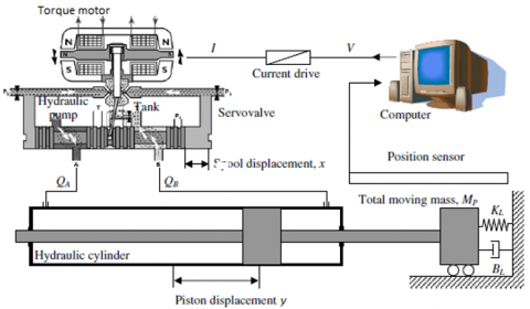
This section deals with the detailed modeling of the Electrohydraulic Servo Actuator (EHSA) and its subsystems-the electromagnetic torque motor, two-stage electrohydraulic servo valve incorporating flapper valve amplifier with mechanical feedback, and the actuating cylinder as shown in Figure 1. The definitions and the numerical values of the overall model equations are collected and tabulated in Appendix-A.
Figure 1. Physical Scheme of EHSA
The dynamic behavior of the EHSA system is described by a set of mathematical relations. Due to this complicated system, there are some assumptions are taken into consideration in the model:
•The pressure losses of the transmission lines are neglected.
•The jet reaction forces are neglected.
•The pressure supply in the system is constant.
•The effect of flow forces and armature hysteresis are neglected.
•The hydraulic cylinder is ideal without friction.
2.1 Electromagnetic torque motor
The electromagnetic torque motor transforms a low-level electric input signal into a mechanical torque that is proportionate to it. The net torque is influenced by the flapper rotational angle and the effective input current. The following torque expression can be derived by ignoring the impact of magnetic hysteresis.
$T=K_i i_e+K_\theta \theta$ (1)
2.2 Armature equation of motion
$T=J \ddot{\theta}+f_\theta \dot{\theta}+K_T \theta+T_L+T_P+T_F$ (2)
$T_P=\frac{\pi}{4} d_f^2\left(P_2-P_1\right) L_f$ (3)
2.2.1 Feedback torque
The feedback torque TF depends on the spool displacement x and the flapper rotational angle $\theta$, as given by the following equations:
$T_F=F_s L_s$ (4)
$T_F=K_s L_s\left(L_s \theta+x\right)$ (5)
where, Fs is the force acting at the extremity of the feedback spring, $F_s=K_s\left(L_s \theta+x\right)$.
2.2.2 Flapper position limiter
The flapper displacement is limited mechanically by the jet nozzles. When reaching any of the side nozzles, the seat reaction develops a counter torque, given by the following equation:
$T_L= \begin{cases}0 & \left|x_f\right|<x_i \\ R_s \dot{\theta}-\left(\left|x_f\right|-x_i\right) K_{L f} L_f & \left|x_f\right|>x_i\end{cases}$ (6)
2.3 Flow rates through the flapper valve restrictions
The flow rates through the flapper valve restrictions are given by the following equations:
$Q_1=C_d A_0 \sqrt{\frac{2\left(P_s-P_1\right)}{\rho}}$ (7)
$Q_2=C_d A_0 \sqrt{\frac{2\left(P_s-P_2\right)}{\rho}}$ (8)
$Q_3=C_d \pi d_f\left(x_i+x_f\right) \sqrt{\frac{2\left(P_1-P_3\right)}{\rho}}$ (9)
$Q_4=C_d \pi d_f\left(x_i-x_f\right) \sqrt{\frac{2\left(P_2-P_3\right)}{\rho}}$ (10)
$x_f=L_f \theta$ (11)
$Q_5=C_d A_5 \sqrt{\frac{2\left(P_3-P_t\right)}{\rho}}$ (12)
2.4 Continuity equations applied to the flapper chambers
The general mathematical expression of the continuity equation is $\sum Q_{\text {in }}-\sum Q_{\text {out }}=\frac{V}{B} \frac{d P}{d t}$. The application of the continuity equation to the flapper valve chambers results in the following relations:
$Q_1-Q_3+A_s \dot{x}=\frac{V_0-A_s x}{B} \frac{d P_1}{d t}$ (13)
$Q_2-Q_4-A_s \dot{x}=\frac{V_0+A_s x}{B} \frac{d P_2}{d t}$ (14)
$Q_3+Q_4-Q_5=\frac{V_3}{B} \frac{d P_3}{d t}$ (15)
2.5 Equation of motion of the spool
The motion of the spool valve is described by the following equation:
$A_s\left(P_2-P_1\right)=m_s \ddot{x}+f_s \dot{x}+K_s L_s \theta+K_s x$ (16)
2.6 Flow rates through the spool valve
Neglecting the effect of transmission lines, connecting the valve to the symmetrical cylinder, the flow rates through the valve restrictions areas are given by:
$Q_a=C_d A_a \sqrt{\frac{2\left(P_A-P_t\right)}{\rho}}$ (17)
$Q_b=C_d A_b \sqrt{\frac{2\left(P_s-P_A\right)}{\rho}}$ (18)
$Q_c=C_d A_c \sqrt{\frac{2\left(P_s-P_B\right)}{\rho}}$ (19)
$Q_d=C_d A_d \sqrt{\frac{2\left(P_B-P_t\right)}{\rho}}$ (20)
The valve restriction areas are given by:
$\left.\begin{array}{r}A_a=A_c=\omega c \\ A_b=A_d=\omega \sqrt{\left(x^2+c^2\right)}\end{array}\right\}$ for $x \geq 0$ (21)
$\left.\begin{array}{r}A_b=A_d=\omega c \\ A_a=A_b=\omega \sqrt{\left(x^2+c^2\right)}\end{array}\right\}$ for $x \leq 0$ (22)
2.7 Continuity equations applied to the cylinder chambers
Applying the continuity equation to the cylinder chambers, considering the internal leakage, and neglecting the external leakage, the following equations were obtained:
$Q_b-Q_a-\frac{\left(P_A-P_B\right)}{R_i}-A_p \dot{y}=\frac{V_c+A_p y}{B} \frac{d P_A}{d t}$ (23)
$Q_c-Q_d+\frac{\left(P_A-P_B\right)}{R_i}+A_p \dot{y}=\frac{V_c-A_p y}{B} \frac{d P_B}{d t}$ (24)
where, the internal leakage $Q_i=\frac{\left(P_A-P_B\right)}{R_i}$.
Figure 2. SIMULINK block diagram of the EHSA
2.8 Equation of motion of the piston
The motion of the piston under the action of pressure, viscous friction, inertia, and external forces is described by the following equation:
$A_P\left(P_A-P_B\right)=m_p \ddot{y}+f_p \dot{y}+K_b y$ (25)
2.9 Feedback system
The piston displacement is picked up by a position sensor and feedback to the electronic controller, which generates the corresponding error signal. The feedback loop can be described by the following equations:
$i_e=i_c-i_b$ (26)
$i_b=K_{F B} y$ (27)
The Simulink block diagram of the EHSA system with internal leakage obtained from Equations (1) to (27) is shown in Figure 2. The boundary conditions used would depend on the specific characteristics and requirements of the system being modeled.
The control strategies that will be developed in this paper are Proportional-Integral-Derivative (PID) controller, Sliding Mode Controller (SMC), and a hybrid control algorithm sliding mode-PID (SMCPID) controller. The main function of the control method is to enhance the overall performance of the system represented in the motion control with insuring the stability of the system.
3.1 PID controller design
The proportional-Integral-Derivative (PID) controller is the most generic form of feedback. It was an essential element of early governors. PID controller is used in more than 95 % of process control loops nowadays. The PID controllers are today found in all areas where control is used [37]. The PID algorithm is described by:
$u(t)=K_P e(t)+K_i \int_0^t e(t) d t+K_d \frac{d e(t)}{t}$ (28)
where,
KP=proportional gain
Ki=Integral gain
Kd=Derivative gain
e(t)=error of the system
The error signal e(t) is the difference between the instantaneos values of the input signal (desired state) and the output signal (feedback signal) as illustrated by Figure 3.
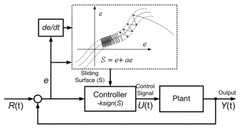
3.2 Sliding mode control (SMC)
SMC is developed in early sixty’ in Russia [38] and has become an efficient tool in the control of complex systems with disturbances due to its low sensitivity to uncertainties and parameter variations. The basic concept of SMC design is shown schematically in Figure 4. The main idea behind SMC is to use a discontinuous control input to force the state trajectory onto a certain well known sliding surface (S=0) and to remain on this surface over time. The design of the SMC consists of two main steps: including the design of the slide surface and the design of the control law [39].
Figure 3. PID controller structure
Figure 4. SMC controller structure
3.2.1 Sliding surface control
The design of the sliding surface is important to develop a realistic but stabilized sliding surface S for the system error states. Defining the EHSA position error e, velocity error $\dot{e}$, acceleration error $\ddot{e}$, and the acceleration derative error $\dddot{e}$. $y_r$ is the given reference input signal, according to equation (25), (26), and (27), can be expanded as:
$e=y_r-y$ (29)
$\dot{e}=\dot{y}_r-\dot{y}$ (30)
$\ddot{e}=\ddot{y}_r-\ddot{y}$ (31)
$\dddot{e}=\dddot{y}_x-\dddot{y}$ (32)
$\dddot{e}=\dddot{y}_r-\frac{-1}{m_p^2}\left(\left(f_p\left(A_p\left(P_A-P_B\right)+i_e \frac{k_b}{k_{F B}}\right)+\left(k_b m_p-f_b^2\right) \dot{y}-f_b \frac{k_b}{k_{F B}} u(t)\right)\right)$ (33)
The sliding surface, s(t) used in this work is described by:
$s(t)=\left(\lambda+\frac{d}{d t}\right)^{n-1} \times e(t)$ (34)
where,
$\lambda$=positive constant
n=model order of the EHSA
Therfore, the sliding surface, s for the third order EHSA system is considered as follows:
$s=\ddot{e}+2 \lambda \dot{e}+\lambda^2 {e}$ (35)
So, the deravitive of the sliding surface, $\dot{s}$ can be expressed as:
$\dot{s}=\dddot{e}+2 \lambda \ddot{e}+\lambda^2 \dot{e}$ (36)
The general expression of SMC control structure, $u_{s m c}(t)$ consists of switching control and equivalent control as shown in equation (37). The switching control, $u_{sw}(t)$ is obtained at $s(t) \neq 0$ corresponding to the reaching phase. While the equivalent control, $u_{e q}(t)$ is obtained at $s(t)=0$ corresponding to the sliding phase.
$u_{s m c}(t)=u_{e q}(t)+u_{s w}(t)$ (37)
3.2.2 Sliding mode control design
The first expression $s(t)=0$ was used in the sliding surface design. The second expression $\dot{s}=0$ will be used in the control design. So, the equivalent control $u_{e q}(t)$ can be obtained by substituting equation (33) into equation (36), we will get:
$u_{e q}(t)=\frac{1}{C_1}\left[\dddot{y}_r+C_2+C_1 i_e+C_3 \dot{y}+2 \lambda \ddot{e}+\lambda^2 \dot{e}\right]$ (38)
where, $C_1=\frac{f_b k_b}{k_{F B} m_p^2}, C_2=\frac{f_b A_p}{m_p^2}\left(P_A-P_B\right), C_3=\frac{k_b m_p-f_p^2}{m_p^2}$.
By applying the sign function to the sliding surface, the switching control $u_{s w}(t)$ can be described by:
$u_{s w}(t)=\eta \operatorname{sign}(s)$ (39)
where, $\eta$ is positive constant value and sign(s) is the signum function which described by the following:
${sign}(s)= \begin{cases}1 & \text { at } s(t)>0 \\ 0 & \text { at } s(t)=0 \\ -1 & \text { at } s(t)<0\end{cases}$ (40)
3.2.3 Lyapunov stability theorem
The Lyapunov theorem, as described in [48], was used to verify the controller's stability using the following Lyapunov function:
$V(t)=\frac{1}{2} s^2(t)$ (41)
where, $V(t)>0$ and $V(0)=0$ for $s(t) \neq 0$. To ensure the stability condition defined by the trajectory moving from the reaching phase to the sliding phase, the reaching condition is described as:
$\dot{V}(t)=s(t) \dot{s}(t)<0$, for $s(t) \neq 0$ (42)
Substituting by equations (33), (36), (37), and (39) into equation (42), this will yield to:
$\begin{aligned} s(t) \dot{s}(t) & =s(t)\left(\dddot{e}+2 \lambda \ddot{e}+\lambda^2 \dot{e}\right)<0=s\left(\dddot{y}_r-\frac{-1}{m_p^2}\left(f_p\left(A_p\left(P_A-P_B\right)+i_{\varepsilon} \frac{k_b}{k_{F B}}\right)\right.\right. \\ & \left.+\left(k_b m_p-f_b^2\right) \dot{y}-f_b \frac{k_b}{k_{F B}}\left(u_{e q}(t)+u_{s w}(t)\right)+2 \lambda \ddot{e}+\lambda^2 \dot{e}\right)<0\end{aligned}$ (43)
Then,
$s(t) \dot{s}(t)=s(t)\left[-C_1 u_{s w}(t)\right]=-s(t) C_1 \eta \,\,{sign}(s)=-C_1 \eta|s(t)|<0$ (44)
To assure the stability of the switching control based on the Lyapunov theory, the chattering phenomenon of the discontinuous signum function in equation (39) has been decreased by replacing the following hyperbolic tangent function as presented in [40].
$u_{s w}(t)=\eta \tanh \left(\frac{s}{\varphi}\right)$ (45)
where $\varphi$ is the boundary layer of the hyperbolic tangent function.
Finally, the total control signal of the SMC is the summation of the two equations (38) and (45) as follow:
$u_{s m c}(t)=\frac{1}{C_1}\left[\begin{array}{c}\dddot{y}_r+C_2+C_1 i_e \\ +C_3 \dot{y}+2 \lambda \ddot{e}+\lambda^2 \dot{e}\end{array}\right]+\eta \tanh \left(\frac{s}{\varphi}\right)$ (46)
3.3 Hybrid (SMCPID) controller
This section deals with the design of a hybrid control algorithm sliding mode-PID (SMCPID) controller. The sliding surface for this controller will be as follows:
$s(t)=\left(k_p+k_i \int_0^t d t+k_d \frac{d}{d t}\right)^{n-1} \times e(t)$ (47)
For the third order EHSA system, n=3, we will get:
$s=\left(k_p^2+2 k_d k_i\right) e+2 k_p k_i \int_0^t e d t+2 k_p k_d \dot{e}+k_i^2\left(\int_0^t e d t\right)^2+k_d^2 \ddot{e}$ (48)
So, the derivative of the sliding surface, $\dot{s}$ can be expressed as:
$\dot{s}=\left(k_p^2+2 k_d k_i\right) \dot{e}+2 k_p k_i e+2 k_p k_d \ddot{e}+k_i^2 \int_0^t e d t+k_d^2 \dddot{e}$ (49)
By substituting equation (33) into equation (49), we will get:
$u_{e q}(t)=\frac{1}{k_d^2 C_1}\left(k_d^2\left(\dddot{y}_r+C_2+C_1 i_e+C_3 \dot{y}\right)+\left(k_p^2+2 k_d k_i\right) \dot{e}+2 k_p k_i e+2 k_p k_d \ddot{e}+k_i^2 \int_0^t e d t\right)$ (50)
where, $C_1=\frac{f_b k_b}{k_{F B} m_p^2}, C_2=\frac{f_b A_p}{m_p^2}\left(P_A-P_B\right), C_3=\frac{k_b m_p-f_p^2}{m_p^2}$.
To verify the stability of the controller using the Lyapunov function in equation (41), we will substitute equations (33), (37), (39), and (49) into equation (42), this will yield to:
$\begin{gathered}s(t) \dot{s}(t)=s(t)\left(\left(k_p^2+2 k_d k_i\right) \dot{e}+2 k_p k_i e+2 k_p k_d \ddot{e}+k_i^2 \int_0^t e d t+k_d^2 \dddot{e}\right)<0 \\ =s\left(\left(k_p^2+2 k_d k_i\right) \dot{e}+2 k_p k_i e+2 k_p k_d \ddot{e}+k_i^2 \int_0^t e d t+k_d^2\left(\dddot{y}_r-\frac{-1}{m_p^2}\left[f_p\left(A_p\left(P_A-P_B\right)+i_e \frac{k_b}{k_{F B}}\right)+\right.\right.\right. \\ \left.\left.\left.\left(k_b m_p-f_b^2\right) \dot{y}-f_b \frac{k_b}{k_{F B}}\left(u_{e q}(t)+u_{s w}(t)\right)\right]\right)\right)<0\end{gathered}$ (51)
Then,
$s(t) \dot{s}(t)=s(t)\left[-C_1 k_d^2 u_{s w}(t)\right]=-s(t) C_1 k_d^2 \eta {~sign}(s)=-C_1 k_d^2 \eta|s(t)|<0$ (52)
From equations (44) for SMC and equation (52) for SMCPID, we can check the stability condition $\dot{V}(t)<0$ as follow:
•When $s>0$, so ${sign}(s)=1>0$,, then equations (44) and (52) wille be $\dot{V}(t)=s(t) \dot{s}(t)<0$.
•When $s>0$, so ${sign}(s)=-1<0$,, then equations (44) and (52) wille be $\dot{V}(t)=s(t) \dot{s}(t)<0$.
From above, this asserts that the design switching control from equation (39) will be stable for $s>0$ and $s<0$. Based on that the Lyapunov stability theorem is being used to guide the design of SMC and SMCPID controllers for the third order EHSA system, and the system output will be bound when the input is bound.
Finally, the total control signal of the hybrid SMCPID controller is the summation of the two equations (50) and (45) as follow:
$u_{s m c p i d}(t)=\frac{1}{k_d^2 C_1}\left(k_d^2\left(\dddot{y}_r+C_2+C_1 i_e+C_3 \dot{y}\right)+\left(k_p^2+2 k_d k_i\right) \dot{e}+2 k_p k_i e+2 k_p k_d \ddot{e}+k_i^2 \int_0^t e d t\right)+\eta \tanh \left(\frac{s}{\varphi}\right)$ (53)
Although the PID, SMC, hybrid SMCPID controllers have good control performance for electrohydraulic servo systems, if the parameters are not appropriate, it will result in failure to track, significant tracking error, chattering, and other problems. As a result, the optimization algorithm is used in this paper to optimize the controller parameters. The PSO was introduced in 1995 by James Kennedy and Russell Eberhart [41]. It was designed using the swarm intelligence of fish schooling and bird flocking movement Behavior to locate food.
A swarm of individuals known as particles flows across a high-dimensional search space with a defined position and velocity to the global optimal solution (maximum or minimum). Each particle in the swarm provides an excellent solution and follows a basic concept by reproducing its previous success. Furthermore, the personal best position in a neighborhood affects the particle position, and the optimal solution between personal best positions is known as the global best position [42]. Let Xi and Vi represent the ith particle position and its corresponding velocity in search space. The best previous position of ith particles recorded and represented as Pbi. The best particle from all the particles in the group is represented as Gb.
The updated velocity of ith individual is given as:
$V_i^{k+1}=w^k V_i^k+c_1 r_1\left(P b_i^k-X_i^k\right)+c_2 r_2\left(G b^k-X_i^k\right)$ (54)
And the next generation values as follows:
$X_i^{k+1}=X_i^k+V_i^{k+1}$ (55)
where,
$V_i^{k+1}$=Velocity of the ith individual at iteration k
wk=Inertia weight at iteration k
c1, c2=Cognitive and social acceleration factors
r1, r2=Uniform random numbers between 0 and 1
$X_i^{k}$=Position of the ith individual at iteration k
$Pb_i^{k}$=Best position of the ith individual at iteration k
Gbk=Best position of the group until iteration k
The overall design process using the PSO algorithm is illustrated in the flow chart as shown in Figure 5.
Figure 5. Flow chart of PSO algorithm [29]
In this paper the initialization parameters of the optimization process are shown in Table 1. The dimension of the optimiz.ation problem is 3, 2, and 2 for PID, SMC, and the hybrid SMCPID controllers, respectively. In addition, the inertia weighting coefficient w is set to be linearly decreased from 1.2 to 0.9 as proposed by the researcher in reference [43]. Integral-square-error (ISE) criteria will be used as an objective/fitness function that used to calculate the minimum error produced in each iteration as shown:
$I S E=\int_0^{\infty} e(t)^2 d t$ (56)
Table 1. The initialization parameters of PSO algorithm
|
Initialization Parameters |
Value |
|
Particles population size (Generation), G |
10 |
|
Number of maximum iterations, k |
20 |
|
Cognitive acceleration factors, c1, |
2 |
|
Social acceleration factors, c2 |
2 |
The simulation program is designed with numerical values from a typical electro-hydraulic servo actuator (EHSA) in mind, as shown in Appendix-A. The dynamic performance and transient response of the EHSA system are described by the equations (1) to (27). These equations reflect a sophisticated non-linear mathematical modelling of the system, which was utilized to create a computer simulation program with the MATLAB/SIMULINK R2022b package. The boundary conditions used by the simulation program are a step input current of 6 mA with a step time of 0.2 seconds, the piston loading coefficient of 1000 N/m, supply pressure of 250 bar, and return pressure 0 bar. The EHSA system response is over-damped with a reference value of 3 mm, rise time of 0.3696 second, overshoot of 0.496 % and with root mean square (RMS) error of 5.584x10⁻³. The transient response of the EHSA is shown in Figure 6.
Figure 6. Step response of the EHSA without controller
It shown from the simulation result that the EHSA system has a slow response with large steady state error. To overcome this, three controllers are used to ensure better performance for the EHSA system.
Table 2. Control parameters
|
Controller |
Control Parameters |
|||||
|
Kp |
Ki |
Kd |
$\lambda$ |
$\phi$ |
$\eta$ |
|
|
PID |
25 |
0.63 |
0.024 |
--- |
--- |
--- |
|
SMC |
9.2 |
0.318 |
0.0932 |
50 |
253.75 |
2.16 |
|
SMCPID |
7.54 |
0.136 |
0.0027 |
--- |
253.66 |
2.39 |
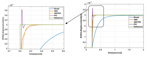
The implementation of PID, SMC, and the hybrid SMCPID controllers to the EHSA are shown in Figure 7. The control parameters for the three types of controllers are summarized in Table 2.
Figure 7. Step response of the EHSA with controller
Table 3. Transient response analysis of the controlled EHSA
|
Controller |
Performance Indexes |
|
|
O.S% |
RMS (x10-3) |
|
|
Model |
0.496 |
5.584 |
|
PID |
21.37 |
1.413 |
|
SMC |
0.364 |
1.156 |
|
SMCPID |
0.426 |
1.013 |
A through analysis for the controlled system transient response is carried out, and the results are shown in Table 3, where the root mean square error (RMS) values, overshoot percentage (O.S %) are calculated and act as the performance indexes for comparison purposes as follow:
$R M S E=\sqrt{\sum_{i=1}^n \frac{\widehat{y}_l-y_i}{n}}$ (57)
$\%$ overshoot $=\exp \left(\frac{-\eta \pi}{\sqrt{1-\eta^2}}\right) \times 100 \%$ (58)
From results, the implementation of the controllers to the EHSA model improve the performance of the system. It is possible to infer from the data that the hybrid SMCPID, SMC, and PID controllers improve MSE by 81.86%, 79.29%, and 74.69% respectively. While the controllers have a different impact on the overshoot percentage. Indeed, we need to apply an optimization technique to obtain the accurate control parameters that provide an overall best performance of the EHSA system.
Figure 8(a). Implementation of PSO algorithm on PID
Figure 8(b). Implementation of PSO algorithm on SMC
Figure 8(c). Implementation of PSO Algorithm on hydrid SMCPID
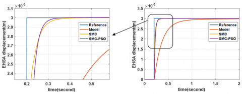
The Particle Swarm Optimization (PSO) is applied to the PID, SMC, hybrid SMCPID controllers based on the algorithm explained in section 4. The initializing parameters are taken from Table 1. The dimension of the optimization problem is 3, 2, and 2 for PID, SMC, and the hybrid SMCPID controllers, respectively. In addition, the inertia weighting coefficient w is set to be linearly decreased from 1.2 to 0.9. the Integral-square-error (ISE) criteria will be used as an objective/fitness function that used to calculate the minimum error produced in each iteration. From the simulation results, Figure 8 (a), (b), and (c) show the effect of implementation the utilized PSO algorithm individually on the PID, SMC, and the hybrid SMCPID controllers. The optimization parameters used in the optimization process are summarized in Table 4.
A through analysis for the optimized system transient response is carried out, and the results are shown in Table 5 according to equations (57) and (58).
Table 4. Optimization parameters of PSO algorithm
|
Controller |
Parameters |
|||||
|
Kp |
Ki |
Kd |
$\lambda$ |
$\phi$ |
$\eta$ |
|
|
PID-PSO |
22.34 |
0.52 |
0.0038 |
--- |
--- |
--- |
|
SMC-PSO |
7.2 |
0.6 |
0.01 |
50 |
143.75 |
1.13 |
|
SMCPID-PSO |
8.2 |
0.2 |
0.0025 |
--- |
194.97 |
1.24 |
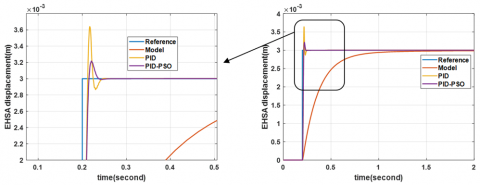
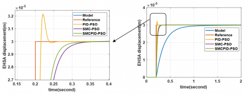
From the results, the utilized PSO algorithm provides a great impact to the system response. It can be infered that the hybrid SMCPID, SMC, and PID controllers improve MSE by 82.34%, 81.37%, and 75.43 respectively. Figure 9 shows the effect of using PSO to the PID, SMC, hybrid SMCPID controllers. Thus, it can concluded that the hybrid SMCPID controller optimized through PSO algorithm generates the best performance of the EHSA according to the performance indexes values of the overshoot percentage and the MSE by 0.408% and 0.986x10⁻³ respectively.
Table 5. Transient response analysis of the optimized EHSA
|
Controller |
Performance indexes |
|
|
O.S% |
RMS (x10-3) |
|
|
Model |
0.496 |
5.584 |
|
PID-PSO |
6.989 |
1.372 |
|
SMC-PSO |
0.415 |
1.04 |
|
SMCPID-PSO |
0.408 |
0.986 |
Figure 9. Implementation of PSO algorithm
Over the past few years, the electrohydraulic servo actuators (EHSA) Technology has been one of the most sought-after research subjects in the industrial and academic fields. In this study, a non-linear mathematical model of the EHSA system is built and three types of controllers; PID, SMC, and a hybrid control algorithm sliding mode-PID (SMCPID) controller are designed. Then, the PSO algorithm optimized the control scheme is implemented to the system which the Lyapunov theorem has been used to verify its stability condition. The transient response and the controller tracking performance is compared where the root mean square error (RMS) values, overshoot percentage (O.S %) are calculated and function as the performance indexes for comparison purposes. The numerical simulations clearly inferred that the proposed hybrid control algorithm sliding mode-PID (SMCPID) controller tuned by PSO technique outperforms the PID and SMC controllers in terms of overall performance.
The Numerical Values of the Studied System
Torque motor
Current-torque gain $K_i=0.556 {Nm} / A$
Armature damping coefficient $f_\theta=0.002 {Nms} / {rad}$
Armature moment of inertia $J=5 \times 10^{-7} {kg}\,\, {m}^2$
Armature rotational angle gain $K_\theta=5 \times 10^{-7}{Nm} / {rad}$
Servoactuator feedback gain $K_{F B}=2 {A} / {m}$
Flexible tube rotational stiffness $K_T=10 {N} / {m}$
Flapper valve
Flapper length $L_f=9 {mm}$
Mechanical feedback spring length $L_s=30{mm}$
Flapper limiting displacement $x_i=30 \mu m$
Flapper nozzle diameter $d_f=0.5{mm}$
Equivalent flapper seat material damping coefficient $R_s=5000 {Nsm} / {rad}$
Flapper seat equivalent stiffness $K_{L f}=5 \times 106 {N} / {m}$
Hydraulic amplifier nozzles N1 & N2 diameter $d_f=0.5 {mm}$
Diameter of the return orifice $N 5, d_5=0.6 {mm}$
Hydraulic oil
Oil density $\rho=867 {kg} / {m}^3$
Bulk modulus os oil $B=1.5 {GPa}$
Spool valve
Spool diameter $d_s=4.6 {mm}$
Initial volume of oil in spool side chamber $V_o=2 {cm}^3$
Initial Volume of oil in the return chamber $V_3=5 {cm}^3$
Spool mass $m_s=0.02 {kg}$
Spool port width $\omega=2 {mm}$
Spool radial clearance $c=2 \mu m$
Spool Damping coefficient $f_s=2 {Ns} / {m}$
Feedback spring stiffness $K_s=900 {N} / {m}$
System pressures
Supply Pressure $P_s=250{bar}$
Return Pressure $P_t=0{bar}$
Hydraulic Cylinder
Piston area $A_p=12.5 {cm}^2$
Initial volume of oil in cylinder chamber $V_c=100 {cm}^3$
Resistance to internal leakage $R_i=1014 {Pas} / {m}^3$
Piston mass $m_p=10{kg}$
Friction coefficient on piston $f_p=1000 {Ns} / {m}$
Piston loading coefficient $K_y=100 {N} / {m}$
[1] Adnan, R., Tajjudin, M., Ishak, N., Ismail, H., Rahiman, M.H.F. (2011). March. Self-tuning fuzzy PID controller for electro-hydraulic cylinder. In 2011 IEEE 7th International Colloquium on Signal Processing and its Applications, IEEE, Penang, Malaysia: 395-398. http://dx.doi.org/10.1109/CSPA.2011.5759909
[2] Izzuddin, N.H., Johari, M.R., Osman, K. (2015). System identification and predictive functional control for electro-hydraulic actuator system. In 2015 IEEE International Symposium on Robotics and Intelligent Sensors (IRIS), Langkawi, Malaysia: 138-143. IEEE. http://dx.doi.org/10.1109/IRIS.2015.7451600
[3] Vo, C.P., Dao, H.V., Ahn, K.K. (2021). Robust fault-tolerant control of an electro-hydraulic actuator with a novel nonlinear unknown input observer. IEEE Access, 9: 30750-30760. https://doi.org/10.1109/ACCESS.2021.3059947
[4] Inderelst, I.M., Prust, I.D., Siegmund, M. (2020). Electro-hydraulic SWOT-analysis on electro-hydraulic drives in construction machinery. Dresden: Technische Universität Dresden, 3: 225-237.
[5] Miao, J., Wang, J., Wang, D., Miao, Q. (2021). Experimental investigation on electro-hydraulic actuator fault diagnosis with multi-channel residuals. Measurement, 180: 109544. https://doi.org/10.1016/j.measurement.2021.109544
[6] Rahmat, M.F.A., Zulfatman, Z., Husain, A.R., Ishaque, K., Sam, Y.M., Ghazali, R., Rozali, S.M. (2011). Modeling and controller design of an industrial hydraulic actuator system in the presence of friction and internal leakage. International Journal of the Physical Sciences, 6(14): 3502-3517. https://doi.org/10.5897/IJPS11.546
[7] Gdoura, E. K., Feki, M., Derbel, N. (2015). Sliding mode control of a hydraulic servo system position using adaptive sliding surface and adaptive Gai. International Journal of Modelling Identification and Control, 23(3): 248-259. http://dx.doi.org/10.1504/IJMIC.2015.069946
[8] Othman, S.M., Rahmat, M.F., Rozali, S.M., Salleh, S. (2015). Review on sliding mode control and its application in electrohydraulic actuator system. Journal of Theoretical and Applied Information Technology, 77(2): 199-208.
[9] Liu, Z., Lu, X., Gao, D. (2019). Ship heading control with speed keeping via a nonlinear disturbance observer. The Journal of Navigation, 72(4): 1035-1052. https://doi.org/10.1017/S0373463318001078
[10] Adel, Z., Hamou, A.A., Abdellatif, S. (2018). October. Design of Real-time PID tracking controller using Arduino Mega 2560 for a permanent magnet DC motor under real disturbances. In 2018 International Conference on Electrical Sciences and Technologies in Maghreb (CISTEM), Algiers, Algeria: 1-5.
[11] Pourebrahim, M., Ghafari, A.S., Pourebrahim, M. (2016). Designing a LQR controller for an electro-hydraulic-actuated-clutch model. In 2016 2nd International Conference on Control Science and Systems Engineering, Singapore: 82-87. https://doi.org/10.1109/CCSSE.2016.7784358
[12] Aly, M., Roman, M., Rabie, M. and Shaaban, S. (2017). Observer-based optimal position control for electrohydraulic steer-by-wire system using gray-box system identified model. Journal of Dynamic Systems, Measurement, and Control, 139(12): 121002. https://doi.org/10.1115/1.4037164
[13] Ahmed, M.I., Azad, A.K.M. (2016). Mathematical modeling and DLQR based controller design for a non-minimum phase Electro Hydraulic Servo system (EHS). In 2016 IEEE Region 10 Conference (TENCON), Singapore: 1839-1844. https://doi.org/10.1109/TENCON.2016.7848339
[14] Ba, D.X., Ahn, K.K. (2016). An optimal controller for an electro-hydraulic system. In 2016 16th International Conference on Control, Automation and Systems (ICCAS), Gyeongju, Korea (South): 167-172. https://doi.org/10.1109/ICCAS.2016.7832315
[15] Puglisi, L.J., Saltaren, R.J., Garcia, C., Banfield, I.A. (2015). Robustness analysis of a PI controller for a hydraulic actuator. Control Engineering Practice, 43: 94-108. https://doi.org/10.1016/j.conengprac.2015.06.010
[16] Fadel, M.Z., Rabie, M.G., Youssef, A.M. (2019). Modeling, simulation and control of a fly-by-wire flight control system using classical PID and modified PI-D controllers. Journal Européen des Systèmes Automatisés, 52(3): 267-276. http://dx.doi.org/10.18280/jesa.520307
[17] Yang, X., Zheng, X., Chen, Y. (2017). Position tracking control law for an electro-hydraulic servo system based on backstepping and extended differentiator. IEEE/ASME Transactions on Mechatronics, 23(1): 132-140. https://doi.org/10.1109/TMECH.2017.2746142
[18] Bayrak, A., Tatlicioglu, E., Zergeroglu, E. (2018). Backstepping control of electro-hydraulic arm. In 2018 6th International Conference on Control Engineering & Information Technology (CEIT), Istanbul, Turkey: 1-4. https://doi.org/10.1109/CEIT.2018.8751833
[19] Li, S., Wang, W. (2020). Adaptive robust H∞ control for double support balance systems. Information Sciences, 513: 565-580. https://doi.org/10.1016/j.ins.2019.10.006
[20] Jing, W.X., Zhen, L.M., Shuai, C., Hao, L., Wang, X. (2019). PID-PFC control of continuous rotary electro-hydraulic servo motor applied to flight simulator. The Journal of Engineering, 2019(13): 138-143. https://doi.org/10.1049/joe.2018.8984
[21] Liang, X.W., Ismail, Z.H. (2019). System identification and model predictive control using CVXGEN for electro-hydraulic actuator. International Journal of Integrated Engineering, 11(4): 166-171. http://dx.doi.org/10.30880/ijie.2019.11.04.018
[22] Essa, M.E.S.M., Aboelela, M.A., Moustafa Hassan, M.A., Abdrabbo, S.M. (2019). Model predictive force control of hardware implementation for electro-hydraulic servo system. Transactions of the Institute of Measurement and Control, 41(5): 1435-1446. http://dx.doi.org/10.1177/0142331218784118
[23] Mahapatra, S.D., Saha, R., Sanyal, D., Sengupta, A., Bhattacharyya, U., Sanyal, S. (2016). Designing low-chattering sliding mode controller for an electrohydraulic system. In 2016 IEEE First International Conference on Control, Measurement and Instrumentation (CMI), Kolkata, India: 316-320. https://doi.org/10.1109/CMI.2016.7413762
[24] Nguyen, M.T., Dang, T.D., Ahn, K.K. (2019). Application of electro-hydraulic actuator system to control continuously variable transmission in wind energy converter. Energies, 12(13), 2499. https://doi.org/10.3390/en12132499
[25] Cheng, L., Zhu, Z.C., Shen, G., Wang, S., Li, X., Tang, Y. (2019). Real-time force tracking control of an electro-hydraulic system using a novel robust adaptive sliding mode controller. IEEE Access, 8: 13315-13328. https://doi.org/10.1109/ACCESS.2019.2895595
[26] Lee, D., Song, B., Park, S.Y., Baek, Y.S. (2019). Development and control of an electro-hydraulic actuator system for an exoskeleton robot. Applied Sciences, 9(20): 4295. https://doi.org/10.3390/app9204295
[27] Liu, Y. and Handroos, H. (1999). Technical note sliding mode control for a class of hydraulic position servo. Mechatronics, 9(1): 111-123.
[28] Bonchis, A., Corke, P.I., Rye, D.C. (2002). Experimental evaluation of position control methods for hydraulic systems. IEEE Transactions on Control Systems Technology, 10(6): 876-882.
[29] Ghani, M.F., Ghazali, R., Jaafar, H.I., Soon, C.C., Sam, Y.M. and Has, Z., 2022. Improved Third Order PID Sliding Mode Controller for Electrohydraulic Actuator Tracking Control. Journal of Robotics and Control (JRC), 3(2): 219-226. https://doi.org/10.1016/S0957-4158(98)00044-0
[30] Mpanza, L.J. and Pedro, J.O. (2016). Sliding mode control parameter tuning using ant colony optimization for a 2-DOF hydraulic servo system. In 2016 IEEE International Conference on Automatic Control and Intelligent Systems, Selangor, Malaysia, pp. 242-247. https://doi.org/10.1109/I2CACIS.2016.7885322
[31] Essa, M.E.S.M., Aboelela, M.A., Hassan, M.A. (2017). A comparative study between ordinary and fractional order PID controllers for modelling and control of an industrial system based on Genetic Algorithm. In 2017 6th International Conference on Modern Circuits and Systems Technologies, Thessaloniki, pp. 1-4. https://doi.org/10.1109/MOCAST.2017.7937622
[32] Yao, J., Wan, Z., Fu, Y., Sheng, T., Yang, M. (2018). An artificial bee colony algorithm for solving hydraulic shaking table acceleration harmonic estimation problem. In Noise Control and Acoustics Division Conference, Chicago, Illinois, USA, pp. V001T08A001. https://doi.org/10.1115/NCAD2018-6105
[33] Li, J., Chen, Q. (2015). Fractional order controller designing with firefly algorithm and parameter optimization for hydroturbine governing system. Mathematical Problems in Engineering, 2015: 825608. https://doi.org/10.1155/2015/825608
[34] Rahmat, M.F., Othman, S.M., Rozali, S.M., Has, Z. (2018). Optimization of modified sliding mode control for an electro-hydraulic actuator system with mismatched disturbance. In 2018 5th International Conference on Electrical Engineering, Computer Science and Informatics (EECSI), Malang, Indonesia, pp. 1-6. https://doi.org/10.1109/EECSI.2018.8752807
[35] Wu, J., Huang, Y., Song, Y., Wu, D. (2019). Integrated design of a novel force tracking electro-hydraulic actuator. Mechatronics, 62: 102247. https://doi.org/10.1016/j.mechatronics.2019.06.007
[36] Jia, L. and Zhao, X. (2019). An improved particle swarm optimization (PSO) optimized integral separation PID and its application on central position control system. IEEE Sensors Journal, 19(16): 7064-7071. https://doi.org/10.1109/JSEN.2019.2912849
[37] Fadel, M.Z., Rabie, M.G., Youssef, A.M. (2019). Motion control of an aircraft electro-hydraulic servo actuator. IOP Conference Series: Materials Science and Engineering, 610: 012073. https://doi.org/10.1088/1757-899X/610/1/012073
[38] Edwards, C., Spurgeon, S. (1998). Sliding mode control: theory and applications. Crc Press.
[39] Lin, Y., Shi, Y., Burton, R. (2011). Modeling and robust discrete-time sliding-mode control design for a fluid power electrohydraulic actuator (EHA) system. IEEE/ASME Transactions on Mechatronics, 18(1): 1-10. https://doi.org/10.1109/TMECH.2011.2160959
[40] Eker, I. (2010). Second-order sliding mode control with experimental application. ISA Transactions, 49(3): 394-405. https://doi.org/10.1016/j.isatra.2010.03.010
[41] Eberhart, R. and Kennedy, J. (1995). Particle swarm optimization. In Proceedings of the IEEE International Conference on Neural Networks, Perth, WA, Australia, 1942-1948. https://doi.org/10.1109/ICNN.1995.488968
[42] Pillay, N. (2008). A particle swarm optimization approach for tuning of SISO PID control loops. Master’s Degree, Durban University of Technology Department of Electronic Engineering.
[43] Shi, Y., Eberhart, R. (1998). A modified particle swarm optimizer. In 1998 IEEE international conference on evolutionary computation proceedings. IEEE World Congress on Computational Intelligence, Anchorage, AK, USA. pp. 69-73. https://doi.org/10.1109/ICEC.1998.699146