Outdoor Localization for a Mobile Robot under Different Weather Conditions Using a Deep Learning Algorithm

Mobile robots are equipped to perform human service roles, either because the tasks are challenging or hazardous [1] or simply because of ease of use [2]. Mobile robots are used in agriculture [3], military applications [4], and medical activities. For example, the outbreak of the coronavirus illness (COVID-19) in 2020 accelerated the process to industries the autonomous robots [5]. One of the most important aspects of mobile robots is navigation [6]. In some conditions, localization provided success in navigation.

The problem of localization in the mobile robot is the estimation in the operating area of the location and orientation of the autonomous mobile robot. The location of the robot depends upon the sensor used. Odometry, RGB, Light Detection and Ranging (LiDAR), Global Position System (GPS), laser radar, ultrasonic, infrared, and microwave are the sensors widely used for mobile robots [7].

Due to varying environmental conditions, some methods declined to classify a mobile robot's position accurately. Furthermore, specific sensors, for example RGB, did not perform admirably in an outdoor setting where light is empathetic. Other approaches are affected in rainy or textured environments. As a result, a system dependent on 3-D data and a DL technique was proposed to obtain precision and durability in identifying the precise position of the mobile robot in various weather conditions. In addition, a robust CNN architecture with thousands of datasets has been proposed with differences in the data collection environment.

There are three levels in the suggested process. Each level contains a variety of activities, including training level, testing level, and classification level. The PCA technique is used to convert a 3D LiDAR point cloud scan into a 2.5-D image during the training level. The Convolution Neural Network (CNN) algorithm is used to extract features from the 2.5-D images., Then, to include them in the classification level, all features and point cloud data are saved as a matrix. This is for determining the proper ground location of a mobile robot. Image fusion is performed at the testing level by merging two pictures, RGB and Depth, into a single RGB-D fusion image and then features extraction from the RGB-D fusion image using CNN. In the classification level, the tested image is classified using the K-Nearest Neighbors algorithm to identify the location of a mobile robot.

The novelty of this paper is to improve outdoor localization in mobile robots using 3-D data from LiDAR and RGB-D, using the proposed system of PCA method, KNN algorthim, and deep learning algorithm.

This paper is structured as follows: The related work in Section 2. In section 3, the material and methodology are presented. the proposed method is outlined in details in section 4. The experimental results and discussion are presented in Section 5. Finally, section 6 gives the conclusion.

To train the deep learning network and obtain the 3D dataset, two sensors are used mounted with the mobile robot; LiDAR and RGB with Depth (RGB-D) sensor.

3.1 Point cloud LiDAR sensor

The data obtained by a LiDAR is used to create 3D models and maps of structures and environments. LiDAR determines the structure by measuring the time it takes for signals to bounce off surfaces and return to the scanner [18]. After analysing and organising the individual readings, the LiDAR data becomes point cloud data. The point clouds are vast arrays of 3D elevation points with x, y, and z coordinates [14]. A standard 3D LiDAR is from the other hand, may acquire surroundings data with a vertical Field of View (FOV) of 30 (±15) º and a horizontal FOV of 360º at a scanning rate of about 10 Hz [14]. High resolution allows the LiDAR to gather a large amount of valuable data in a region of long ranges. LiDAR is commonly used in robot systems because of these advantages [14].

3.2 Reduction 3D LiDAR point cloud to 2.5D image

One of the most well-known and widely utilized methods is Principal Component Analysis (PCA). Its premise is straightforward: limit the dimensionality of a dataset while retaining as much 'variability' (i.e., statistical information) as possible [19]. Solving the covariance matrix obtains the major components. The PCs of the PCA space are calculated in this method in two steps. The data matrix's covariance matrix (X) is constructed first. Second, the covariance matrix's eigenvalues and eigenvectors are determined. The covariance matrix is asymmetric and always positive semi-definite matrix (i.e., X= XT). The variable variance is represented by the diagonal values xi, I= 1,..., M of the covariance matrix, whereas the off-diagonal entries as illustrated in Equation (1), represent the covariance between two separate variables. A positive covariance matrix value shows A positive correlation between two variables is indicated by a positive value, a negative correlation is indicated by a negative value, and a zero value indicates that the two factors are uncorrelated or statistically independent [20].

$\left(\begin{array}{cccc}\operatorname{Var}\left(\mathrm{x}_1, \mathrm{x}_1\right) & \operatorname{Cov}\left(\mathrm{x}_1, \mathrm{x}_2\right) & \ldots & \operatorname{Cov}\left(\mathrm{x}_1, \mathrm{x}_{\mathrm{M}}\right) \\ \operatorname{Cov}\left(\mathrm{x}_2, \mathrm{x}_1\right) & \operatorname{Var}\left(\mathrm{x}_2, \mathrm{x}_2\right) & \ldots & \operatorname{Cov}\left(\mathrm{x}_2, \mathrm{x}_{\mathrm{M}}\right) \\ \vdots & \vdots & \ddots & \vdots \\ \operatorname{Cov}\left(\mathrm{x}_{\mathrm{M}}, \mathrm{x}_1\right) & \operatorname{Cov}\left(\mathrm{x}_{\mathrm{M}}, \mathrm{x}_2\right) & & \operatorname{Var}\left(\mathrm{x}_{\mathrm{M}}, \mathrm{x}_{\mathrm{M}}\right)\end{array}\right)$                (1)

The eigenvalues ($\lambda$) and eigenvectors (V) of the covariance matrix are calculated based [20]:

$V \Sigma=\lambda V$             (2)

The first principal component has the most giant variance and is represented by the eigenvector with the highest eigenvalue. Each eigenvector corresponds to a single primary component. The eigenvectors depict the directions in the PCA space [21].

3.3 Ground removal by rotation around Z-axis

In 3D, there are a variety of techniques to express rotations. Euler angles, quaternions, and rotation matrices are common representations. Even though they require various parameters, these representations can describe rotations with three degrees of freedom [22, 23]:

$\mathrm{R}_{\mathrm{z}}=\left[\begin{array}{ccc}\cos (\theta) & -\sin (\theta) & 0 \\ \sin (\theta) & \cos (\theta) & 0 \\ 0 & 0 & 1\end{array}\right]$           (3)

$\mathrm{R}_{\mathrm{x}}=\left[\begin{array}{ccc}1 & 0 & 0 \\ 0 & \cos (\theta) & -\sin (\theta) \\ 0 & \sin (\theta) & \cos (\theta)\end{array}\right]$            (4)

$\mathrm{R}_{\mathrm{y}}=\left[\begin{array}{ccc}\cos (\theta) & 0 & \sin (\theta) \\ 0 & 1 & 0 \\ -\sin (\theta) & 0 & \cos (\theta)\end{array}\right]$             (5)

3.4 RGB-D camera

Because of popular RGB-D sensors such as Microsoft's Kinect, showing 3D data as RGB-D images has really become popular in recent years. RGB-D data provides a 2.5D representation of the captured 3D object by including a depth map (D) as well as 2D color information (RGB). Although cheap, RGB-D data are simple yet effective representations of 3D objects that can be used for various tasks such as identity recognition, pose regression, and scene reconstruction [24, 25].

3.5 Fusion image by (IHS) Transformations

Image fusion is a technique used to extract useful data from many input photographs and merge it to create a new output image that is more descriptive and useful than the sum of the input images [26]. Image fusion reduces data size, keeps vital features, and provides a more accessible image [27].

The IHS methodology has become a standard process in image processing for color enhancement, feature enhancement, pixel size optimization, and the merging of various data sets. The goal of combining high-resolution and hyperspectral remotely sensed photos is to ensure spectral data while also including high - spatial detail information, making the fusion significantly more suitable for IHS treatment [28]. Because the RGB to IHS conversion model employs a 3x3 matrix as its transform kernel, most literature considers IHS to be a third-order process. Most literature considers IHS to be a third-order process. Many published studies indicated that different IHS transformations are used, which have significant variations in the matrix values, as described below. R = Red, G = Green, and B = Blue were used in this analysis. I = Intensity, H = Hue, S = Saturation, and V1, V2 = Cartesian hue and saturation elements [28].

$\begin{gathered}{\left[\begin{array}{c}I \\ V_1 \\ V_2\end{array}\right]=\left[\begin{array}{ccc}\frac{1}{\sqrt{3}} & \frac{1}{\sqrt{3}} & \frac{1}{\sqrt{3}} \\ \frac{-1}{\sqrt{6}} & \frac{-1}{\sqrt{6}} & \frac{2}{\sqrt{6}} \\ \frac{-1}{\sqrt{2}} & \frac{1}{\sqrt{2}} & 0\end{array}\right]\left[\begin{array}{l}R \\ G \\ B\end{array}\right] H=\tan ^{-1}\left(\frac{\mathrm{V} 2}{\mathrm{~V} 1}\right) \mathrm{S}=} \sqrt{V_1^2+V_2^2}\end{gathered}$            (6)

The RGB and depth pictures are merged in the precise location to form the 2.5D image in IHS methods. The color-carrying data is detached from the intensity variable in a color picture (Hue and Saturation). The IHS color is created by utilizing geometrical formulas to convert RGB points into matching points [29].

3.6 Deep learning algorithms

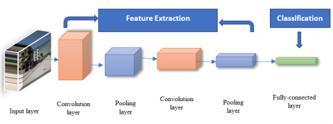
Machine learning has taken a powerful turn in recent years, thanks to the rise of Artificial Neural Networks [30]. One of most impressive forms of ANN architecture is CNN [31]. The CNN is a hybrid of artificial neural networks and cutting-edge deep learning techniques. CNN's are at the heart of spectacular developments in deep learning. For decades, this artificial neural network has been used to perform various image detection tasks. CNN has recently piqued the interest of researchers from around the world, as it has demonstrated impressive results in a variety of computer vision and machine learning tasks [32]. As depicted in Figure 1, CNNs are built up of three layers: Convolution, pooling, and fully connected layers. Convolution and pooling are the first two layers that extract features, whereas the third, a fully connected layer, maps specific features into the outcome, such as classification. A convolution layer, a type of linear operation, is a crucial aspect of CNN. It is made up of a set of mathematical operations such as convolution. Image pixels are stored in a two-dimensional matrix [33].

1.png

Figure 1. The architecture of CNN [32]

3.7 K-Nearest Neighbour (K-NN) algorithm

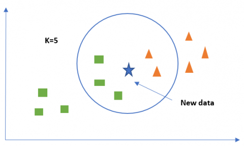
For data classification tasks, distance-based algorithms are commonly used. One of the most widely used distance-based algorithms is the K-Nearest Neighbor classification (K-NN). This classification calculates the distances between the testing machine and the training data to decide the final classification performance. With numerical results, the standard K-NN classifier works well [34]. A popular distance-based classification method is the K-Nearest Neighbour's (K-NN) classification technique. The standard K-NN classification algorithm recognises the K-Nearest Neighbor(s) and categorizes numerical data records by measuring the distance between both the test sample and all training samples using the Euclidian distance [35].

1. Calculate the number of closest neighbours (K values); see Figure 2.

2. As indicatedin Figure 3, find the distance between both the testing data and one of the training examples.

The proximity between $\mathrm{A}$ and $\mathrm{B}$ in Euclidean$

\text { distance }=\sqrt{\left(X_2-X_1\right)^2+\left(Y_2-Y_1\right)^2}

$         (7)

2.png

Figure 2. K-Nearest neighbor principle [34]

3. Sort the distance using the K-th minimal distance to find the nearest neighbours.

4. Make a list of the categories of your nearest neighbours.

5. Use the simple majority of the group of closest neighbors as the additional data object's prediction value. neighbours.

3.png

Figure 3. The Euclidian distance to measure the distance between two data [35]

3.8 Measuring the error

To calculate the error of an approximate arithmetic circuit. The Error Rate (ER), Mean Square Error (MSE), and Mean Error Distance (MED) are used to calculate the error rate. For example, the discrepancy between the estimated and real sums S* and S is known as the error of distance (ED) [36]:

$E D=\left|S^*-S\right|$          (8)

The error rate is the number of input configurations for which the predicted adder produces wrong outputs (ER). As a result, a non-zero error gap can be calculated as:

$\mathrm{ER}=\mathrm{P}(\mathrm{ED} \neq 0)$            (9)

The (MED) is the average of all error distances. The Mean Squares of Error (MSE) overall error distances is calculated as [36]:

$\mathrm{MED}=\mathrm{E}[\mathrm{ED}]=\sum_{\mathrm{ED}_{\mathrm{i}} \in \Omega} \mathrm{ED}_{\mathrm{i}} \mathrm{P}\left(\mathrm{ED}_{\mathrm{i}}\right)$            (10)

$M S E=E\left[E D^2\right]=\sum_{\mathrm{ED}_i \in \Omega} E D_{\mathrm{i}}^2 \mathrm{P}\left(\mathrm{ED}_{\mathrm{i}}\right)$            (11)

where, Ω is the total number of error distances.

MSE is calculated as follows: if n predictions are made from a sample of n data, Y is the variable being forecasted, and Y ̂ is the predicted value [37]:

MSE $=\frac{1}{n} \sum_{i=1}^n\left(Y_i-\widehat{Y}_i\right)^2$                 (12)

5.1 Collected datasets

Using supervised learning, typically, a large amount of data is required to train a neural network. To train and test the proposed system, a dataset that included Image data in different weather conditions, depth images, and LiDAR data with corresponding mode labels was used. Seeing as this was not realized in the public domain, it was decided to employ a simulator to generate the data required. Simulated results are created using the CARLA driving simulator. CARLA is a testing simulator for autonomous vehicles (open-source simulator) [38]. CARLA was explicitly built to support the production, training, and testing of self-driving automated systems. CARLA also offers available digital assets (urban layouts, homes, and automobiles) built specifically for this purpose and can be widely accessed [38, 39]. A camera sensor can be attached to a mobile robot in CARLA to capture images at a fixed frame rate. As seen in Figure 5, the camera sensor can produce images in both RGB and Depth.

5-1.png

(a) RGB image

5-2.png

(b) Depth image

Figure 5. The RGB image corresponds to the Depth map (photos from Carla open-source simulator)

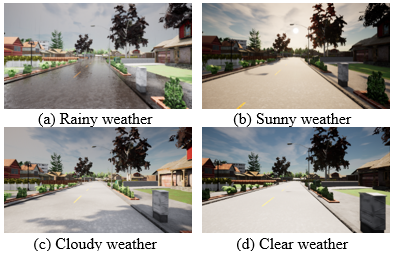
The simulator is capable of simulating a variety of weather conditions. Rain with puddles light reflected, cloud cover that darkens the ambience, and simulated sunny weather that produces fake lens flares whereas the sun is in the frame are all examples. In addition, data on a variety of environmental conditions is collected [38], seen in Figure 6.

66.png

Figure 6. Image visualization in a variety of weather conditions (photos from Carla open-source simulator)

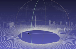
LiDAR sensors can be reproduced in CARLA. The upper and lower farms of view, as well as the number of channels, total size, and the number of points in each direction can be customized. During scan capture, the simulation region can be frozen, resulting in a 360-degree scan without the need for velocity adjustments. Figures 7 and 8 are two examples of this.

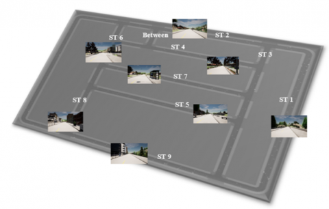
To create the data sets used in this study, a mobile robot equipped with LiDAR sensor and RGB-D camera was set to travel around a map on autopilot. The data set encompasses roughly 120,000 m2 of a map, including the suburban neighbourhoods, downtown area, and wooded areas. Two training data sets were obtained, one with 15000 images, 5000 images for each weather condition and Depth picture pairs, and 46,741 LiDAR frames. As seen in Figure 9, this city district is divided into nine streets with a street between them.

Each street has two sections: the begin and the end, as seen in Table 1.

7.png

Figure 7. LiDAR scan as a point cloud (photos from Carla open source simulator)

8.png

Figure 8. LiDAR analysis after MeshLab display [38]

9.png

Figure 9. Carla simulator's suggested street numbers

5.2 CNN localization

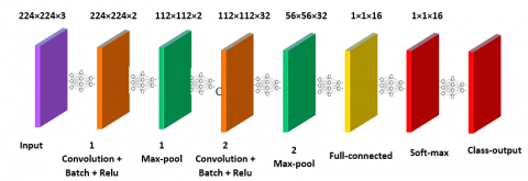
The CNN for localization has a total of 12 layers. With a brief training period, a 12-layer CNN with a 224 x 224 input image was designed. The optimizer Stochastic Gradient Descent with Momentum (SGDM) was used in this network. Table 2 shows the analysis result of the network design. With the K-NN classifier, there are 16 classes based on the number of streets identified in Figure 9.

Figure 10 illustrates the configuration of the implemented CNN.

10.png

Figure 10. CNN localization with 12-layers

Table 1. Division of streets and data for each street

Table 2. Analysis result for the CNN architecture

	Name	Type	Activations	Learnables
1	Imageinput 224×224×3 image with ‘zerocenter’ normalization	Image input	224×224×3	-
2	CONV_1 2 3×3×2 convolutions with stride [1 1] and padding [1 1 1 1]	Convolution	224×224×2	Weights 3×3×3×2 Bias       1×1×2
3	Batchnorm_1 Batch normalization with two channels	Batch Normalization	224×224×2	offset   1×1×2 scale    1×1×2
4	Relu_1 ReLU	ReLU	224×224×2	-
5	Maxpool_1 2×2 max pooling with stride [2 2] and padding [0 0 0 0]	Max Pooling	112×112×2	-
6	CONV_2 32 3×3×2 convolutions with stride [1  1] and padding [1  1  1  1]	Convolution	112×112×32	Weights 3×3×2×32 Bias      1×1×32
7	Batchnorm_2 Batch normalization with 32 channels	Batch Normalization	112×112×32	offset   1×1×32 scale    1×1×32
8	Relu_2 ReLU	ReLU	112×112×32	-
9	Maxpool_2 2×2 max pooling with stride [2 2] and padding [0 0 0 0]	Max Pooling	56×56×32	-
10	FC 16 fully connected layer	Fully Connected	1×1×16	Weights 16×100352 Bias       16×1
11	Softmax softmac	Softmax	1×1×16	-
12	Classoutput Crossentropex with ‘between’ and 15 other classes	Classification output	-	-

11.jpg

Figure 11. The result of training time expended and training accuracy

5.3 Network training and analysis

The MatLab code was created on a PC equipped with a Core (TM) Intel (R) i5-8250U processor. 1.80 GHz RAM 8 GB, UHD Graphics 620. It took four epochs to process the dataset containing 46,741 LiDAR frames. Each epoch has 70 iterations, with a maximum of 280 iteration numbers possible and a learning period rate of 3*10^-4. The preparation took 415 minutes, containing 70% of the dataset for training and 30% of the test dataset. As seen in Figure 11, the accuracy obtained is 97.46%.

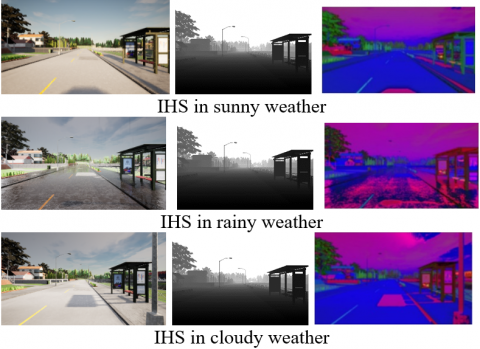
5.4 Result of IHS transformation

When merging RGB and Depth images, the IHS method has an impact. The Intensity of a pixel in a depth picture varies based on its brightness. Figure 12 shows how the Hue, Saturation, and Intensity combine in the 2.5-d images in various weather conditions. The change in the 2.5D images is noticed for these three different weather conditions, which led to the strength of the approach in identifying the mobile robot's correct position in these weather changes.

12.png

Figure 12. Creating a 2.5D image by merging two RGB with different conditions and depth images

5.5 Evaluation results

To check the performance of the proposed approach of PCA method with IHS and using the K-NN algorithm, it is necessary to obtain a high-quality and precise localization sample that can be compared to reality on the ground. Tested nine states with random locations in the city under different weather conditions are listed in Table 3:

Table 3. Summary of test results in various weather conditions (Cloudy, Rainy and Sunny weather)

State	The correct localization prediction	MSE
1	Between streets	0.0432
2	Beginning of street 1	0.0472
3	Beginning of street 2	0.0421
4	Street 6	0.0360
5	End of street 9	0.036
6	Street 3	0.0216
7	End of street 1	0.0545
8	End of street 5	0.0678
9	Street 6	0.036
Mean error		0.0427

Table 4. A comparison of the proposed method to other methods

Method	Average error	Maximum error	Training time	Data set
Fingerprinting positioning method + IEEE802.11a platform, i.e., 5 GHz in ISM band [40]	20.12 m	20.12 m	--	--
Particle filter based on Monte Carlo Localization [17]	0.6 m	2.7 m	-	16530 images
ICP+ PointNetLK+ GoogleNet [23]	18.3 m	131.6 m	4200 minutes	10400 images
Proposed method CNN +PCA +K-NN	0.6 m	1.09 m	415 minutes	46741 frame LiDAR

CARLA achieved a frame rate of 30 frames per second (FPS) in one meter to calculate the Mean Error Distance. From equations (10 and 11), MED = 0.6 meters.

The proposed approach is superior to the research method is depicted in Table 4.

Table 4 reference 40 used the technique positioning system WifiLOC, which is currently being developed as a research tool at the University of Zilina. WifiLOC estimates a mobile device's location using RSS information from nearby Wi-Fi APs. The method is built on the fingerprinting positioning algorithm and earlier RSS data. The proposed approach does not rely on a picture of deep learning technologies, so the error rate is respectively high. In reference 17, Only use a stereo camera for vision-based localization in outdoor environments. A particle swarm optimization based on Monte Carlo Localization is used in the localization process, which fails in extreme cases. For example, due to the camera's restricted dynamic range, direct sunlight will saturate a significant portion of the captured image to black or white. Researchers discovered that this problem is equivalent to wheel slip in wheel odometry and categorized it as an abducted robot problem to overcome this limitation. It also notes that the average error is almost equal to the proposed method, but the maximum error is 2.7 m, and the proposed method does not exceed 1.09 m. While in reference 23, the (ICP) algorithm was used, the PointNetLK network was utilized in registration, and GoogleNet was used for the RGB-D Neural network. Also, notice that average error and training time are very high compared to the proposed method. The proposed system used a deep learning technique that took 415 minutes to train. Although the dataset was 46,741 LiDAR frames to obtain the accuracy of 97.46%, MSE equals 0.0427, and the Mean Error of Distance equals 0.6 meters using the PCA method for the fusion picture IHS is used the K-NN classifier. The findings of the proposed work reduce the training time, are more accurate, and reduce the error rate.