Youcef Islam Djilani Kobibi* | Mohamed Abdeldjalil Djehaf | Mohamed Khatir
© 2022 IIETA. This article is published by IIETA and is licensed under the CC BY 4.0 license (http://creativecommons.org/licenses/by/4.0/).
OPEN ACCESS
The modular multilevel converter (MMC) is a recently developed converter architecture with the potential for high-voltage direct current (HVDC) transmission applications. Due to the large number of IGBTs and diode devices, modeling a modular multilevel converter (MMC) for electromagnetic transient type (EMT-type) simulations might be difficult. HVDC-MMC transmission system detailed models take a long time to compute. To solve this issue, simplified and averaged models have been suggested. In order to efficiently and accurately depict MMC-HVDC systems, several kinds of models are developed and compared in this study using EMTP-rv software. The results suggest that the kind of model to be used will rely on the study performed and the level of accuracy needed.
HVDC, VSC, MMC, EMTP, average value model, detailed model, switching function
In the latter half of the nineteenth century, direct current was first used commercially for the transfer of electrical power. However, ac electrical power systems came to dominate with the invention of transformers and induction motors about 1890. The supporters of dc and ac systems have long engaged in contentious debates. The widespread use and domination of ac systems could never overcome the clear benefits of dc transmission [1, 2].
When it comes to coupling 50/60 Hz systems, long underground cable systems, long distance bulk power transmission, stable ac interconnection, interties with low short-circuit levels, and high voltage dc (HVDC) transmission, these applications are considered advantageous and, in some cases, superior to ac [1]. For these systems, high voltage ac must be converted to high voltage dc when power is sent, and vice versa at the receiving points. Therefore, the creation of appropriate converters is important to the viability and advantages of an HVDC connection [3].
The modular multilevel converter (MMC), in particular for voltage-sourced converter high-voltage direct current (VSC-HVDC) transmission systems, has emerged as the most intriguing multilevel converter structure for medium/high-power applications [4]. The key benefits of the MMC over other multi-level converter topologies are: 1) its modularity and scalability to meet any voltage level requirements, 2) its high efficiency, which is crucial for high-power applications, and 3) its superior harmonic performance, particularly in high-voltage applications where a lot of identical submodules (SMs) with low-voltage ratings are stacked up, allowing the size of passive filters to be reduced [5].
Modular multilevel converters (MMCs) are used in HVDC and FACTS applications. They incorporate hundreds of SMs [6, 7], which result in a large number of nonlinear IGBT/diode devices.
Previous studies on the MMC-HVDC using EMTP programs are presented by Li et al. [8, 9].
Consequently, it is difficult to simulate such converters for the electromagnetic transient program (EMTP) [6]. HVDC-MMC transmission system detailed models take a long time to compute. To solve this issue, simplified and averaged models have been presented out in the past [7, 10].
This paper's contribution is the comparison of dynamic performance for several MMC model types. This study investigated the dynamic behavior and computational performance for an actual MMC-based HVDC point-to-point transmission system and offers guidance for MMC modeling.
The modular multilevel converter (MMC) topology utilizes the advantages of both the multilevel structure and pulse width modulation (PWM. Low switching losses and low harmonics (high-quality AC voltage) are the results of low effective switching frequency per device, which significantly minimizes the need for filtering [11].
A Sub-Module is the term for MMC's core element (SM). To acquire the necessary output voltage, the number of SM can be either raised or lowered. Half-bridge (HB) converters, full-bridge (FB) converters, a unidirectional sub-module [12], a clamp double (CD) converter sub-module, three level flying capacitors, three level neutral-point, and five level cross-connected SM [13] are all included in the topology of each switching sub-module.
The number and length of the communication links, the network delay, and the tolerance to faults are all significantly influenced by the control network topology. Ring, tree, and hybrid tree-ring topologies appear to have the most promise among the topologies that can be taken into account.
In order to produce a multilevel voltage waveform at the converter terminal, this converter depends on the cell capacitors. To construct a single valve for DC transmission requirements, hundreds of cells are typically needed. The quality of the AC voltage waveform improves and the harmonic content decreases as the level count rises.
The balancing capacity of this architecture is better than the one with NPC converters because it takes advantage of the redundant combination of module connections for each required AC level [14]. The probability of device and/or system failure is decreased since the MMC performs better than the NPC converter under unbalanced operation and symmetrical/asymmetrical AC faults [15]. The MMC is suited for applications subject to strict grid code requirements since it can bypass many forms of AC faults (wind energy). Since there is no common DC capacitor to transfer ripple between phases, if one phase of the AC system experiences a problem, the other two phases of the converter will continue to function normally, maybe at full per-phase power.
These key features, made of the MMC an attractive choice for VSC HVDC transmission system around the world [16], resulting in a rising interest to develop appropriate modeling technics to meet special purpose analysis (control, transient analysis…) and to reduce the simulation time.
When activated by relatively high-frequency signals, the relatively high number of non-linear semiconductors in MMCs poses some difficulties that necessitate a considerable computational power for re-triangularizing the admittance matrix of the electrical power subsystem [16, 17], making the simulation of the MMC occasionally inconvenient when using a traditional modeling method [18].
In order to adress the afore-mentioned difficulties, the research community propose enhanced reduced order models that increase computational efficiency and maintain the targeted accuracy. A recent tendency is to use average value models (AVMs) that are both simple and capable of providing enough accuracy in dynamic simulations. For MMCs, AVMs and other simplified modeling techniques have been provided by Teeuwsen et al. [7, 19-22].
This section tends to classify the modeling methods of the modular multilevel converter. Then, it makes a detailed descriptions and comparisons among the four models in terms of phenomena covering, accuracy, and application. Furthermore, it aims to help the reader to identify and choose the best-suited model for conducting this analysis.
2.1 Full physics-based model
Figure 1. Physics based model for IGBT
Due of the high number of cells, modeling MMCs could become very difficult and simulation could take a long time. Depending on the study type and precision needed, several modeling levels can be attained. Models are introduced in this paper in ascending order of complexity. It is anticipated that model complexity reduction will improve computing performance.
Differential equations or an equivalent circuit serve as representations for each semiconductor device. Models of insulated gate bipolar transistors (IGBTs) can be categorized as either behavior models or physical models [23]. A behavior model can properly depict the properties of the device under specific circumstances despite not being based on physical principles. However, when the device parameters (base width, channel length, gate oxide thickness, etc.) are modified, analytical models [24-31] are able to forecast the IGBT behavior. These factors have a significant impact on how well the device works.
Since a MOS transistor and a BJT can be used to approximate an IGBT, an improved analytical model that uses a single-dimension device simulation model for the BJT and an analytical model for the MOS to develop an IGBT equivalent circuit model was proposed by Kao et al. [28]. This model is compared to earlier physics-based models presented by Baliga et al. [24, 25, 32] and creates the IGBT equivalent circuit model shown in Figure 1.
In the converter design phase, the comprehensive physics-based models are helpful for detailed analysis of the behavior of the semiconductor device and for defining the IGBT's size and doping profile. These models are not typically used for power system studies because they require a very small integration time step (in the order of nanoseconds) in the EMTP in order to accurately depict switching losses. This type won't be covered in the parts that follow because of this.
2.2 Detailed model (nonlinear model)
The ideal controllable switch, one series and one anti-parallel diode, and a snubber circuit [33] are used to depict the anti-parallel IGBT/diode pair in Figure 2. A non-linear resistance is used to depict the diode's non-ideal voltage-current characteristic. The nonlinear characteristic can be modified in accordance with the data provided by the manufacturer.
This model can take into account any MMC conduction method and is the most accurate model for EMT-type programs. The advantages include the ability to perform specific studies like blocked states (g1, g2 OFF), submodule details, the converter start-up sequence, and internal converter faults, as well as improved precision in the modeling of the IGBT/diode pair because the non-linear behavior throughout the switching is included. These models can also be used to assess, tune, and validate less complex MMC models like those mentioned in the following.
Figure 2. Nonlinear IGBT/diode including V-I curve
2.3 Equivalent (or simplified) detailed model
2.3.1 IGBT/Diode representation
This concept is based on the notion that the IGBT device and its anti-parallel diode operate as a bidirectional switch, which is expressed by a two-state resistance, illustrated in Figure 3 by R1 (small conductive value) and R0 (big open-circuit value). This method [17] enables the generation of a Norton equivalent for each MMC arm as well as implementing an arm circuit reduction to remove internal electrical nodes. These two controllable resistances are utilized to swap out the two IGTB/diode combinations. Their values are influenced by capacitor voltage, current direction, and gating signals.
Figure 3. a) IGBT/diode connected in anti-parallel. b) Simplified IGBT/diode model
The IGBT/diode combination may still be thought of as a single two-state resistance, as shown in Figure 4, even if either the diode or the IGBT may be conducting at any one time.
Figure 4. Single two state resistance model
2.3.2 Submodule capacitor representation
By using the trapezoidal formula of integration and Dommel's expression, the capacitor Ccp can be expressed with its Thevenin or Norton equivalents [34]. For the capacitor, the generic Thevenin and Norton equivalents are determined, respectively.
$\begin{aligned} u_{c p}(t) & =\frac{1}{c_{c p}} \int_{t_1-\Delta t}^{t_1} i_{c p}\left(t_1\right) d t+u_{c p}(t-\Delta t) \\ & =R_{c p} . i_{c p}(t)+u_{H i s t}(t-\Delta t)\end{aligned}$ (1)
The voltage across and current through Ccp, respectively, are represented by ucp(t) and icp(t), where Rcp = ∆t/2Ccp. The size of the simulation step is ∆t.
$\begin{aligned} i_{c p}(t) & =\frac{2 C_{c p}}{\Delta t}\left[u_{c p}(t)-u_{c p}(t-\Delta t)\right]-i_{c p}(t-\Delta t) =\frac{u_{c p}(t)}{R_{c p}}+i_{\text {Hist }}(t-\Delta t)\end{aligned}$ (2)
It is clear from (2) that the capacitor can be represented by an equivalent resistance Rcp connected in parallel with the following current source iHist(t-∆t):
$i_{H i s t}(t-\Delta t)=-\frac{u_{c p}(t-\Delta t)}{R_{c p}}-i_{c p}(t-\Delta t)$ (3)
Figures 5 shows the duals of the Thevenin and Norton approximations, which are simply the actual circuit algebraic modifications.
Figure 5. a) The capacitor and its b) Thévenin and c) Norton EMTP equivalents
The electrical representation of the nth SM half-bridge can be shown in Figure 6 [34] using the Thevenin equivalent in (1) for the SM capacitor.
The nth SM output voltage me be written as:
$\begin{aligned} u_{s m o, n} & =\frac{i_{\text {in }}(t)}{1 / R_{2_{-} n}(t)+1 /\left[R_{1_{-} n}(t)+R_{c p}\right]} +\frac{R_{2_{-} n}(t) \cdot u_{\text {Hist }}(t-\Delta t)}{1 / R_{2_{-} n}(t)+1 /\left[R_{1_{-} n}(t)+R_{c p}\right]} =R_{E_{-} n(t)} \cdot i_{i n}(t)+u_{E_{-} n}(t)\end{aligned}$ (4)
Figure 6. EMTP Equivalent model of the Nth half bridge submodule
The capacitor current can be expressed as:
$\begin{aligned} u_{s m o, n} & =\frac{i_{i n}(t)}{1 / R_{2_{-} n}(t)+1 /\left[R_{1_{-} n}(t)+R_{c p}\right]} +\frac{u_{s m, n}(t-\Delta t)+R_c \cdot i_{\mathrm{cp}, n}(t-\Delta t)}{R_{2_{-} n}(t)+R_{1_{-} n}(t)+R_{c p}}\end{aligned}$ (5)
Similarly, the capacitor voltage is calculated as:
$\begin{aligned} u_{s m, n}(t) & =R_{c p} \cdot\left[i_{c p, n}(t)+i_{c p, n}(t-\Delta t)\right] +u_{s m, n}(t-\Delta t)\end{aligned}$ (6)
Thevenin parameters (RE_,n and uE_,n) for the nth submodule are easily obtainable in (4).
2.3.3 Phase arm equivalent
The arm equivalent depicted in Figure 7 is obtained by series connecting the N SMs in the phase arm, where the Thevenin parameters are:
$u_{E_{-,} a r m}(t)=\sum_{n=1}^N u_{E_{-,} \mathrm{n}}(t)$ (7)
$R_{E_{-,} a r m}(t)=\sum_{n=1}^N R_{E_{-,} \mathrm{n}}(t)$ (8)
RE_,n and uE_,n are specified in (4).
Additionally, the model approach described here will need only minor adjustments from the perspective of implementation in order to emulate the full-bridge converter SM [17, 35].
Figure 7. Thevenin equivalent of the MMC VSC-HVDC phase arm
The reduced detailed model is less computationally intensive than the complete detailed models, although being less accurate [36]. This is important for power system research. The main benefit of this kind is the main system of network equations' significant reduction in the number of electrical nodes. It continues to take into account each SM independently and keeps track of the various capacitor voltages and currents. It is applicable to any quantity of SMs within one arm.
2.4 Averaged models
2.4.1 Averaged model based on the switching function
In this model, the switching function Sn notion of a half-bridge converter is used to average each MMC arm. We make the following assumptions: that all MMC internal variables are perfectly under control, that all SM capacitor voltages are perfectly balanced, and that second harmonic circulating currents in each phase are suppressed. The veracity of this assumption increases as the number of SMs per arm and/or the fluctuation amplitudes of capacitor voltages increase. Each arm can be represented in this scenario by a single module, as seen in Figure 8. State-space modeling, with its intrinsic simplicity of manipulation and capacity for frequency domain analysis, is a favoured method for describing dynamic systems. This method can be used to derive an explicit steady-state expression for the circulating current [37-42].
Figure 8. Averaged switching model of the MMC phase arm
If the switching frequency is high enough for the averaging method to be accurate and all of the module parameters and modulation commands are balanced at the module level, this model can capture the information of individual capacitors. However, linear conduction losses and circulating currents can be modeled. For control system methods based on internal MMC energy balance, it is also useful to take into consideration the energy transmitted from the ac and dc sides into each arm of the MMC [43, 44].
This method's clear drawback is that because each arm is reduced to an equivalent switching function model, power switches are no longer represented. This is because the information of the separate modules cannot be identified inside an arm because they are all presumed to be equal.
This modeling approach can be used to research harmonics because it uses longer time steps and substantially less computation time than detailed modeling due to the aforementioned simplifications.
2.4.2 Average model based on fundamental frequency
The switching functions are replaced by reference signals in this model, which duplicates the MMC converter's overall dynamics and suppresses the control blocks. The mathematical formulation is the same as in the previous model. Contrary to [33], the MMC can be depicted as a conventional VSC (2- and 3-level topologies) [45]. Therefore, vref are the voltage references produced by the inner controller [46] using a methodology similar to [47-50]. Figure 9(a) displays this model's ac-side.
Figure 9. Averaged-value model of the MMC converter [48]
The power balancing approach was used to generate the dc-side model in Figure 9(b), which makes no assumptions about energy storage within the MMC converter. The MMC has an inductance in each arm, unlike the traditional VSC model, hence an equivalent inductance should also be supplied on the dc side.
Finally, throughout steady state and dynamic simulations, the two average models that were used in this paper respond satisfactorily. Although the switching function model requires more computation time for the same t, it is more accurate than the typical model based on fundamental frequency. For ac side faults, set point changes, and loss of generation, both the switching model and the AVM can be used to accurately simulate system dynamics.
AVMs can only function properly if the capacitors are big enough to keep the voltage between each MMC submodule roughly constant. The individual capacitor voltages are not estimated, but the large-scale dynamic behavior is adequately represented. An individual dc-side voltage is determined instead.
The four different types of MMC models—DM, EM, SFM, and AVM—are compared in this section. For both standard operation and step-change of active power reference, the dynamic behavior comparison is carried out using EMTP-rv software [10].
Figure 10 shows the system under study. The control approach takes into account dc voltage/reactive power control (VSC 2) and active/reactive power control (VSC 1) on the sending and receiving ends, respectively. The corresponding sources for the ac grids have a shortcircuit level of 10,000 MVA. From VSC1 to VSC2, the system has a 1,000 MW transmission capacity. A wideband line model is used to simulate the DC cable [27]. Every MMC station takes a 101-level MMC (100 SMs/arm) into account. The reference model is the Model 1 (with nonlinear IGBT/diode model). Table 3 in appendix provides parameters of the system of Figure 10 used for the simulation studies.
Figure 10. Point -to-point MMC -HVDC transmission test system
3.1 Steady-state operation
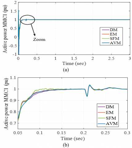
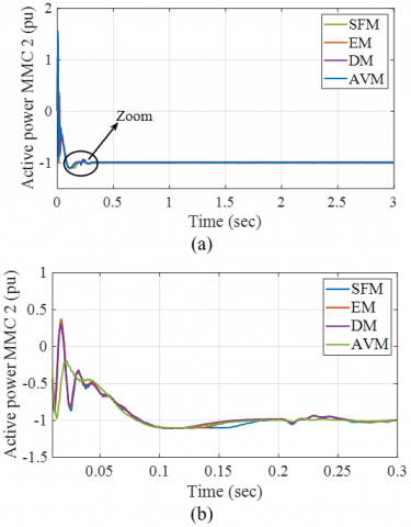
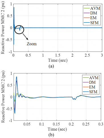
The following Figures 11-15 display the steady-state waveforms that the models for the 1GW MMC-HVDC system produced. The small inaccuracy visible in the zoomed waveform in the following figure confirms that the waveforms are nearly identical. Two converters were simulated to operate at 100MW each as a rectifier and an inverter, respectively. Overall, the results suggest that both converters' active and reactive power precision is good.
Figure 11. Results of simulations in steady state for the four models. Top to bottom: (an Active power at MMC1, (b) Zoomed waveform of active power at MMC1
Figure 12. Results of simulations in steady state for the four models. Top to bottom: (a Reactive power at MMC1, b) Zoomed waveform of reactive power at MMC1
Figure 13. Results of simulations in steady state for the four models. Top to bottom: (a) Active power at MMC2, (b) Zoomed waveform of active power at MMC2
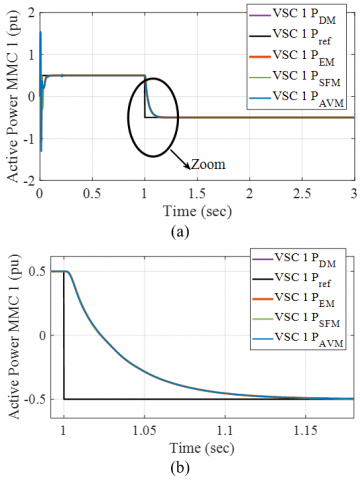
At 1 s of simulation, a step change in the active power reference for VSC 1 is introduced. From 0.5 to -0.5 pu, the active power reference is decreased (power flow reversal). All four models in the figure below produce the same outcomes. In Figure 15, the active power of VSC 1 is shown with the power flow reversed.
Figure 14. Results of simulations in steady state for the four models. Top to bottom: (a Rective power at MMC2, (b) Zoomed waveform of reactive power at MMC2
Figure 15. Step change simulation results for the four models. From top to bottom: (an Active power at MMC1, (b) Zoomed waveform of active power at MMC
Since in Figure 15 both Models EM, SFM and AVM are able to match the results from DM Model, it is concluded that these three simplified models can be used to study converter dynamics. The zoomed waveforms of Figure 15 are used to highlight the accuracy in all models. It is observed that all models mimic the accuracy of DM into the step change on active power reference.
3.2 Computing performance comparison
This section compares the computational capabilities of the many models developed, presented, and reported in Table 1 of this study. The models are contrasted with their elaborated forms. On a machine with a 2.6 GHz Intel Core i5-3230M processor and 4 GB of RAM, the computing performance tests were conducted.
Table 1 displays the simulation performance results for the four models. Computer performance is noticeably faster with the EM. The EM can execute a 3s simulation with a timestep of 10s 56 times faster without sacrificing the precision of the system dynamic response. In terms of computer performance, the averaged models perform better. Using the SFM and AVM, respectively, a simulation of 3s using a time-step of 10s can be completed between 290 and 560 times faster without sacrificing the accuracy of the system's dynamic reaction. When the time-step is raised to 50 s, both the SFM and AVM continue to be suitably accurate. Since the switching valves are not modeled in the AVM, it is possible to employ a slightly larger time-step without sacrificing accuracy, which further increases computational performance. The AVM method can be applied to very large systems and is far faster than DMM. Table 2 lists the benefits, drawbacks, and applicability of each model for various systems investigations [1-3].
Table 1. Computing timings for a 3s simulation
|
Model |
Time-step (µs) |
Time (s) |
|
DM |
10 |
9011.26985 |
|
EM |
10 |
155.56419 |
|
SFM |
10 |
31.29380 |
|
AVM |
10 |
15.1477 |
Table 2. Summary table and comparison of models
|
Features |
DM |
EM |
SFM |
AVM |
|
Harmonics |
Yes |
Yes |
Yes |
No |
|
Accuracy |
Best |
Very Good |
Very good |
Good |
|
Simulation Time |
Very Slow |
Slow |
Fast |
Very Fast |
|
AC Dynamics |
Yes |
Yes |
Yes |
Yes |
|
AC Fast transients |
Yes |
Yes |
Yes |
Yes |
|
DC Side transients |
Yes |
Yes |
Yes/No |
No |
|
VSC Internal faults |
Yes |
No |
No |
No |
|
Resonances |
Yes |
Yes |
Yes |
No |
|
Controls interaction |
Yes |
Yes |
Yes |
Yes |
|
Large systems |
No |
Yes |
Yes |
Yes |
|
Converter Losses |
Best |
Good |
Good |
Good |
The comparison of two MMC modeling methodologies was presented in this paper (Detailed and Averaged Models). It has shown the verification of all models as well as the models in EMTP-rv software. In order to assess modeling methodologies against the DM model technique in terms of accuracy and simulation speed, an MMC-HVDC test system was used. For both steady-state and dynamic performance, the accuracy of the various models was graphically evaluated. These results demonstrate that although all four modeling strategies provide a respectable level of accuracy, the DM is typically the most accurate. It has been demonstrated that the SFM and AVMM models simulate noticeably faster than the DM, while the EM is more computationally effective than the DM. However, the DM model does provide access to SM components (which is not feasible with the EM), thus it might be taken into account when this is a crucial factor.
[1] Ashmore, C. (2006). Transmit the light fantastic [HVDC power transmission]. Power Engineer, 20(2): 24-27. http://dx.doi.org/10.1049/pe:20060204
[2] Willis, L., Stig, N. (2007). HVDC transmission: yesterday and today. Power and Energy Magazine, IEEE, 5(2): 22-31. https://doi.org/10.1109/MPAE.2007.329175
[3] Nami, A., Liang, J., Dijkhuizen, F., Demetriades, G.D. (2015). Modular multilevel converters for HVDC applications: review on converter cells and functionalities. IEEE Transactions on Power Electronics, 30(1): 18-36. https://doi.org/10.1109/TPEL.2014.2327641
[4] Sekiguchi, K., Khamphakdi, P., Hagiwara, M., Akagi, H. (2014). A grid-level high-power BTB (Back-To-Back) system using modular multilevel cascade converters withoutcommon DC-link capacitor. IEEE Transactions on Industry Applications, 50(4): 2648-2659, https://doi.org/10.1109/TIA.2013.2290867
[5] Debnath, S., Qin, J., Bahrani, B., Saeedifard M., Barbosa, P. (2015). Operation, control, and applications of the modular multilevel converter: A review. IEEE Transactions on Power Electronics, 30(1): 37-53. https://doi.org/10.1109/TPEL.2014.2309937
[6] Peralta, J., Saad, H., Dennetiere, S., Mahseredjian J., Nguefeu, S. (2013). Detailed and averaged models for a 401-level MMC-HVDC system. 2013 IEEE Power & Energy Society General Meeting, 27(3): 1501-1508. https://doi.org/10.1109/PESMG.2013.6672356
[7] Teeuwsen, S.P. (2009). Simplified dynamic model of a voltage-sourced converter with modular multilevel converter design, 2009 IEEE/PES Power Systems Conference and Exposition, Seattle, WA, USA, pp. 1-6. https://doi.org/10.1109/PSCE.2009.4839922
[8] Li, X.Y., Li, H., Peng, Y.F., Wang, J.K. (2021). Research on fault ride through control strategy of wind farm via MMC-HVDC networking system. Review of Computer Engineering Studies, 8(4): 95-101. https://doi.org/10.18280/rces.080402
[9] Yahiaoui, A., Iffouzar, K., Ghedamsi, K., Himour, K. (2021). Dynamic performance analysis of VSC-HVDC based modular multilevel converter under fault. Journal Européen des Systèmes Automatisés, 54(1): 187-194. https://doi.org/10.18280/jesa.540121
[10] Saad, H., Jacobs, K., Lin, W., Jovcic, D. (2016). Modelling of MMC including half-bridge and full-bridge submodules for EMT study. 2016 Power Systems Computation Conference (PSCC), Genoa, Italy, pp. 1-7. https://doi.org/10.1109/PSCC.2016.7541008
[11] Jovcic, D., Ahmed, K.H. (2015). High Voltage Direct Current Transmission: Converters, Systems and DC Grids. John Wiley & Sons.
[12] Glasdam, J.B., Zeni, L., Hjerrild, J., Kocewiak, L.H., Hesselbaek, B., Sørensen, P.E., Hansen, A.D., Bak, C.L., Kjaer, P.C. (2013). An assessment of converter modelling needs for offshore wind power plants connected via VSC-HVDC networks. Proceedings of the 12th Wind Integration Workshop: International Workshop on Large-Scale Integration of Wind Power into Power Systems as well as on Transmission Networks for Offshore Wind Plants. Energynautics, London.
[13] Middlebrook, R.D., Cuk, S. (1976). A general unified approach to modelling switching-converter power stages. 1970 IEEE Power Electronics Specialists Conference, Cleveland, OH, USA, pp. 18-34. https://doi.org/10.1109/PESC.1976.7072895
[14] Son, G.T., Lee, H.J., Nam, T.S., Chuang, Y.H., Lee, U.H., Baek, S.T., Hur, K., Park, J.W. (2012). Design and control of a modular multilevel HVDC converter with redundant power modules for noninterruptible energy transfer. IEEE Transactions on Power Delivery, 27(3): 1611-1619. https://doi.org/10.1109/TPWRD.2012.2190530
[15] Adam, G.P., Finney, S.J., Williams, B.W., Ahmed, K.H. (2010). AC fault ride-through capability of VSC-HVDC transmission systems. IEEE Energy Conversion Congress and Exposition (ECCE) Conference, Atlanta, GA, USA. https://doi.org/10.1109/ECCE.2010.5617786
[16] Flourentzou, N., Agelidis V.G., Demetriades, G.D. (2009). VSC based HVDC power transmission systems: An overview. IEEE Transactions on Power Systems, 24(3): 592-602. https://doi.org/10.1109/TPEL.2008.2008441
[17] Gnanarathna, U.N., Chaudhary, S.K., Gole, A., Teodorescu, R. (2010). Modular multi-level converter based HVDC system for grid connection of offshore wind power plant. 9th IET International Conference on AC and DC Power Transmission. London, pp. 1-5. https://doi.org/10.1049/cp.2010.0984
[18] Gnanarathna, U.N., Gole, A., Jayasinghe, R.P. (2011). Efficient Modeling of modular multilevel HVDC converters (MMC) on electromagnetic transient simulation programs. IEEE Transactions on Power Delivery, 26(1): 316-324. https://doi.org/10.1109/TPWRD.2010.2060737
[19] Krein, P.T., Bentsman, J., Bass, R.M., Lesieutre. B.L. (1990). On the use of averaging for the analysis of power electronic systems. IEEE Transactions on Power Electronics, 5(2): 182-190. https://doi.org/10.1109/63.53155
[20] Jin, H. (1997). Behavior-mode simulation of power electronic circuits. IEEE Transactions on Power Electronics, 12(3): 443-452. https://doi.org/10.1109/63.575672
[21] Peralta, J., Saad, H., Dennetiere, S., Mahseredjian, J., Nguefeu, S. (2012). Detailed and averaged models for a 401-Level MMC-HVDC system. IEEE Transactions on Power Delivery, 27(3): 1501-1508. https://doi.org/10.1109/PESMG.2013.6672356
[22] Norrga, S., Angquist, L., Ilves, K., Harnefors, L., Nee, H. (2012). Frequency-domain modeling of modular multilevel converters. IECON 2012 - 38th Annual Conference on IEEE Industrial Electronics Society, pp. 4967-4972. https://doi.org/10.1109/IECON.2012.6389570
[23] Hsu, J.T., Ngo, K.D.T. (1996). Behavioural modeling of the IGBT using the Hammerstein configuration. IEEE Transactions on Power Electronics, 11(6): 746-754. https://doi.org/10.1109/63.542037
[24] Baliga, B.J. (1985). Analysis of insulated gate transistor turn-off characteristics. IEEE Electron Device Letters, 6(2): 74-77. https://doi.org/10.1109/EDL.1985.26048
[25] Hefner, A.R. (1990). Analytical modeling of device-circuit interactions for the power insulated gate bipolar transistor (IGBT). IEEE Transactions on Industry Applications, 26(6): 995-1005. https://doi.org/10.1109/28.62382
[26] Hefner, A.R. (1994). Dynamic electro-thermal model for the IGBT. IEEE Transactions on Industry Applications, 30(2): 364-405. https://doi.org/10.1109/28.287517
[27] Hefner, A.R., Diebolt, D.M. (1994). Experimentally verified IGBT model implemented in the Saber circuit simulator. IEEE Transaction on Power Electronics, 9(5): 532-542. https://doi.org/10.1109/63.321038
[28] Kao, C.H., Tseng, C.C., Liang, Y. (2005). Equivalent circuit model for an insulated gate bipolar transistor. IEE Proceedings on Electrical Power Application. http://dx.doi.org/10.1049/ip-epa:20045151
[29] Sheng, K., Williams, B.W., Finney, S.J. (2000). A review of IGBT models. IEEE Transactions on Power Electronics, 15(6): 1250-1266. https://doi.org/10.1109/63.892840
[30] Huang, T., Gong, J., Chen, S. (2002). Modeling the Turn-off Characteristics of Insulated-Gate Bipolar Transistor. Japanese Journal of Applied Physics, 41(3): 1288-1292. https://doi.org/10.1143/JJAP.41.1288
[31] Yue. Y., Liou, J.J. (1996). An analytical insulated gate bipolar transistor (IGBT) model for steady-state and transient applications under all free-carrier injection conditions. Solid-State Electron, 39(9): 1277-1282. https://doi.org/10.1016/0038-1101(96)00046-9
[32] Kuo, D.S., Hu, C., Sapp, S.P. (1986). An analytical model for the power bipolar-MOS transistor. Solid-State Electron, 29(12): 1229-1237. https://doi.org/10.1016/0038-1101(86)90128-0
[33] Saad, H., Peralta, J., Dennetiere, S., Mahseredjian, J., Jatskevich, J., Martinez, J.A., Davoudi, A., Saeedifard, M., Sood, V.K., Wang, X., Cano, J.M., Mehrizi-Sani, A. (2013). Dynamic averaged and simplified models for MMC-based HVDC transmission systems. IEEE Transactions on Power Delivery, 28(3): 1723-1730. https://doi.org/10.1109/TPWRD.2013.2251912
[34] Dommel, H.W. (1986), EMTP Theory Book, Portland: Bonneville Power Administration.
[35] Peralta, J. (2013). Dynamic averaged models of VSC-based HVDC systems for electromagnetic transient programs, Montreal, Canada: École Polytechnique de Montréal.
[36] Gole, A.M., Keri, A., Kwankpa, C., Gunther, E.W., Dommel, H.W., Hassan, I., Marti, J.R., Martinez, J.A., Fehrle, K.G., Tang, L., McGranaghan, M.F., Nayak, O.B., Ribeiro, P.F., Iravani, R., Lasseter, R. (1997). Guidelines for modeling power electronics in electric power engineering applications. IEEE Transactions Power Delivery, 12(1): 505-514. https://doi.org/10.1109/61.568278
[37] Xu, J., Zhao, C., Liu, W., Guo, C. (2013). Accelerated model of modular multilevel converters in PSCAD/EMTDC. IEEE Transactions on Power Delivery, 28(1): 129-136. https://doi.org/10.1109/TPWRD.2012.2201511
[38] Aghdam, M.G., Gharehpetian, G.B. (2005). Modeling of switching and conduction losses in three-phase SPWM VSC using switching function concept. 2005 IEEE Russia Power Tech, Petersburg, Russia, pp. 1-6. https://doi.org/10.1109/PTC.2005.4524829
[39] Chiniforoosh, S., Jatskevich, J., Yazdani, A., Sood, V.K., Dinavahi, V.R., Martinez, J.A., Ramirez, A. (2010). Definitions and applications of dynamic average models for analysis of power systems. IEEE Transactions on Power Delivery, 25(4): 2655-2669. https://doi.org/10.1109/TPWRD.2010.2043859
[40] Sanders, S.R., Noworolski, J.M., Liu, X.Z., Verghese, G.C. (1991). Generalized averaging method for power conversion circuits. IEEE Transactions on Power Electronics, 6(2): 251-259. https://doi.org/10.1109/63.76811
[41] Peralta, J., Saad, H., Dennetière, S., Mahseredjian J. (2012). Dynamic performance of average-value models for multi-terminal VSC-HVDC systems. IEEE Power and Energy Society General Meeting, pp. 1-8, https://doi.org/10.1109/PESGM.2012.6345610
[42] Qiang, S., Wenhua, L., Xiaoqian, L., Hong, R., Shukai X., Licheng, L. (2013). A steady-state analysis method for a modular multilevel converter. IEEE Transactions on Power Electronics, 28(8): 3702-3713. https://doi.org/10.1109/TPEL.2012.2227818
[43] Munch, P., Gőrges, D., Izak, M., Liu, S. (2010). Integrated current control, energy control and energy balancing of Modular Multilevel Converters. IECON 2010 - 36th Annual Conference on IEEE Industrial Electronics Society, pp. 150-155. https://doi.org/10.1109/IECON.2010.5675185
[44] Antonopoulos, A., Angquist, L., Nee, H. (2009). On dynamics and voltage control of the modular multilevel converter. 2009 13th European Conference on Power Electronics and Applications, Barcelona, Spain, pp. 1-10.
[45] Andersen, B.R., Xu, L., Wong, K.T.G. (2001). Topologies for VSC transmission. International Conference on Ac-dc Power Transmission, London, U.K. https://doi.org/10.1049/cp:20010559
[46] Song, R., Zheng, C., Li, R., Zhou, X. (2005). VSCs based HVDC and its control strategy. 2005 IEEE/PES Transmission & Distribution Conference & Exposition: Asia and Pacific, Dalian, China, pp. 1-6. https://doi.org/10.1109/TDC.2005.1546800
[47] Ouquelle, H., Dessaint, L.A., Casoria, S. (2009). An average value model-based design of a deadbeat controller for VSC-HVDC transmission link. IEEE Power & Energy Society General Meeting. IEEE., Calgary, AB, Canada. https://doi.org/10.1109/PES.2009.5275748
[48] Saad, H.A. (2015). Modélisation et simulation d’une liaison HVDC de type VSC-MMC, Montréal, Canada: École Polytechnique de Montréal.
[49] Beddard, A.J. (2014). Factors affecting the reliability of VSC-HVDC for the connection of offshore windfarms. Manchester: Faculty of Engineering and Physical Sciences, The University of Manchester.
[50] Saad, H., Dufour, C., Mahseredjian, J., Dennetiere, S., Nguefeu, S. (2013). Real time simulation of MMCs using the State-Space nodal approach. IPST International Conference on Power Systems Transients, Vancouver, BC, Canada.