Fezazi Omar* | Abderrahmane Haddj El Mrabet | Imad Belkraouane | Youcef Djeriri
© 2021 IIETA. This article is published by IIETA and is licensed under the CC BY 4.0 license (http://creativecommons.org/licenses/by/4.0/).
OPEN ACCESS
Due to the simple structure of DC motors, the natural decoupling between torque and speed, and its low cost the DC motors have been widely used in electromechanical systems, the paper deals with the experimental method of DC motor Coulomb friction identification that caused the dead nonlinear zone and proposed a nonlinear model of the DC motor, then a sliding mode strategy is developed to control the DC motor in high and low speed for bidirectional operation, The experimental implementation using Dspace 1104 demonstrate that the proposed sliding mode control can achieve favorable tracking performance against non-linearities for a DC motor.
sliding mode control, DC motor, nonlinear, dead zone, Coulomb friction
In general, the DC motor is modeled as a linear system [1], but to get high control performance the need of nonlinear approach is required. The dead zone caused by nonlinear Coulomb friction would bring problems to control the DC motor especially if the system is rotating in two directions or operating at a low speed [2, 3].
Nevertheless, the identification of the parameters of the DCM (direct current motor) is very important to make the speed regulation, but the uncertainty of the measuring devices (amperemeter, voltmeter ....) and the bad use of the identification techniques pose a real problem in order to calculate the PI controller which based on parameters of the DCM. Moreover, the conventional controller performance is affected by unknown load dynamics, changes of speed command, and parameter variations [4, 5] then the choice of an efficient control against these problems and robust against nonlinear dead zone is mandatory.
Sliding mode control seems in a good position to deal with these problems [6-8], it has been used to deal with nonlinear systems [9-11]. This type of control has several advantages such as robustness, precision, stability, and simplicity. This makes it particularly suitable for dealing with systems with poorly known models, either because of parameter identification problems or because of simplification of the system model.
The paper deals at the first with the experimental method of DC motor identification parameters and proposed a nonlinear model of the DC motor, then sliding mode control is simulated by Matlab Simulink to visualize motor speed. Finally, the implementation of sliding mode control (SMC) on DC motor (sonelecRME_24245) is made using Dspace 1104 carte. Simulation and experimental implementation demonstrate that the proposed sliding mode control system can achieve favorable tracking performance against uncertainties and nonlinearities for a DC motor.
Accurate nonlinear model building is a crucial step in practical control problems. The nonlinear model of the DC motor is established in two steps, firstly electrical DCM parameters identification is done like armature resistance and inductance then, mechanical parameters are measured like viscous friction coefficient and total moment of inertia, finally identification of the Coulomb friction torque is done to model the non-linearity of the system [2, 3].
The second step is separate excitation DC motor modeling (DC_sonelecRME_24245 400 Watt), the DCM mechanical part can be modeled as a multi-mass system after electrical part modeling then SLM control is used to control this motor.
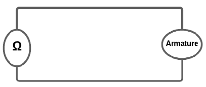
2.1 Armature resistance and inductance identification
To determine the armature resistance Ra, an ohmmeter (TTI1604) is used, which displays the value Ra=9.5Ω. the electrical circuit is shown in Figure 1.
Figure 1. Armature resistance measuring
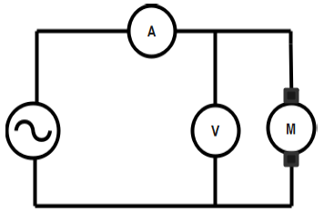
For inductance measurement, the armature is supplied with an AC voltage. the electrical circuit is shown in Figure 2. For different voltage armature values Ua, current armature value Ia is measured to deduce the value of the inductance through the calculation of the average armature impedance Za. Then armature inductance is calculated, the proposed circuit is as follows:
${{L}_{a}}=\frac{1}{2\pi f}\left( \sqrt{Z_{a}^{2}+R_{a}^{2}} \right)={{0.0747049}_{{}}}Henry$ (1)
Figure 2. Armature inductance measuring
Table 1 represents the Calculation armature average impedance.
Table 1. Calculation armature average impedance
|
Ua(V) |
26.31 |
34.72 |
41.1 |
57.5 |
70.7 |
|
I(A) |
1.06 |
1.4 |
1.647 |
2.326 |
2.881 |
|
Z(Ω) |
24.8207547 |
24.8 |
24.9544627 |
24.7205503 |
24.5400902 |
2.2 Viscous friction identification
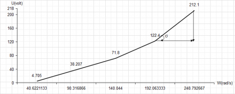
To determine viscous friction, first EMF constant K should be measured, to determine K it is sufficient to perform a no-load test. We measure the voltage U and the velocity Ω to plot the curve $U=f(\Omega)$. Figure 3 allows us to find the value of the constant K.
Figure 3. Curve $U=f(\Omega)$
DCM no-load steady-state electrical equation is:
$\begin{align} & U=R.I+K\Omega \\ & y=ax+b \\ & K=\tan \alpha \\\end{align}$ (2)
So:
$K=\tan \alpha =\frac{212.1-122.4}{248.79-192.06}=1.57$ (3)
DCM no-load steady-state mechanical equation is:
${{C}_{EMF}}={{C}_{f}}\Rightarrow K.I={{f}_{v}}\Omega \Rightarrow {{f}_{v}}=\frac{KI}{\Omega }$ (4)
So:
${{f}_{v}}=\frac{1.57\times 0.296}{192.063}=0.00241962N.m/rad/s$ (5)
2.3 Total moment inertia identification
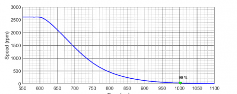
The identification of the parameter J (inertia moment) is done when the machine rotates at a nominal speed, then we cut the power supply on the armature and measure the speed as a function of time Ω=f(t) during the deceleration, then we will take the response time.
Figure 4. Deceleration test curve Ω=f(t)
Figure 4 represent the deceleration test curve after cutting off armature voltage (at 800 ms), DC motor speed decelerates, the response of the DC motor is a first-order response so the mechanical time constant τmec can be calculated after calculating response time ts was taken at 99% of speed maximum value:
$t_{s_{-} 99 \%}=5 * \tau_{\text {mec }}=(1000-800) \mathrm{ms} \Rightarrow \tau_{\text {mec }}=0.08 \mathrm{~s}$ (6)
then J is calculated:
$J=\frac{{{f}_{v}}}{{{\tau }_{mec}}}=\frac{0.0024}{0.08}=0.0302452kg.{{m}^{2}}$ (7)
2.4 Coulomb friction torque identification
In literature, the non-linear Coulomb friction torque is often represented in three different forms, as Coulomb friction is expressed as a sign function depending on the rotation speed [2-12].
Figure 5. Different nonlinear friction models [12]
Figure 5 shows the different representation types that can be made to present Coulomb friction torque which can be written [4]:
$\begin{cases}(a) & C_{c}(\omega)=\alpha \operatorname{sgn}(\omega) \\ (b) & C_{c}(\omega)=\alpha_{0} \operatorname{sgn}(\omega)+\alpha_{1} e^{-\alpha_{2}|w|} \operatorname{sgn}(\omega) \\ (c) & C_{c}(\omega)=\left(\alpha_{0}+\alpha_{1} e^{-\alpha_{2}|w|}\right) \operatorname{sgn} 1(\omega)+\left(\alpha_{3}+\alpha_{4} e^{-\alpha_{5}|w|}\right) \operatorname{sgn} 2(\omega)\end{cases}$ (8)
Figure 5a represents the nonlinear Coulomb friction for systems that operate at high speeds, in this case, Eq. (8.a). express the Coulomb friction as a signum function dependent on the rotational speed [6-13]. The signum function (sgn()) is defined as [6-13]:
$\operatorname{sgn}(\omega)= \begin{cases}1 & \omega \succ 0 \\ 0 & \omega=0 \\ -1 & \omega \prec 0\end{cases}$ (9)
Figure 5b represents the nonlinear Coulomb friction for more accuracy when the system operation is condensed around the zero speed [12, 13] and for systems with very low speeds, in this case, Eq. (8.b). express the Coulomb by an exponential term in velocity [12, 13]. $\propto_{i}$ is defined as a constant real number and i=0, 1, 2, …
Figure 5c represents a generalized model for the nonlinear friction that contain asymmetrical characteristic [13-15]. Where sgn1(ω) and sgn2(ω) are defined as [13]:
$\operatorname{sgn} 1(\omega)= \begin{cases}1 & \omega \geq 0 \\ 0 & \omega \prec 0\end{cases}$ $\operatorname{sgn} 2(\omega)= \begin{cases}0 & \omega \geq 0 \\ -1 & \omega \prec 0\end{cases}$ (10)
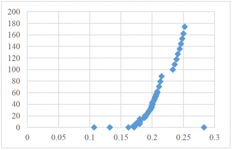
To identify Coulomb friction torque plotting the velocity versus current $\Omega=f(i)$ is done to plot speed as a function of torque $\Omega=f(\mathrm{C})$ to calculate $\alpha $and choose the right non-linear representation seen in the Eq. (8.a).
So Coulomb friction torque can be modeled as Cc(ω)=0.2826 sgn(ω). Figures 6 and 7 represent speed as a function of current and as a function of torque.
Figure 6. Curve Ω=f(Ia)
Figure 7. Curve Ω=f(T)
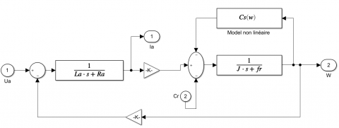
2.5 Block diagram representing the non-linear system
The DCM model is based on two equations electrical and mechanical Eq. (7), Figure 8 presents the block diagram of the non-linear DCM system [5-16].
$\left\{ \begin{align} & {{U}_{a}}-{{R}_{a}}{{I}_{a}}=L\frac{d{{I}_{a}}}{dt}+E\overset{{}}{\mathop {}}\,\overset{{}}{\mathop {}}\,\overset{{}}{\mathop {}}\,\overset{{}}{\mathop {}}\,\overset{{}}{\mathop {}}\,E=K\Omega \\ & J\frac{d\omega }{dt}={{C}_{E}}-{{C}_{f}}-{{C}_{c}}\left( \omega \right)\overset{{}}{\mathop {}}\,\overset{{}}{\mathop {}}\,\overset{{}}{\mathop {}}\,{{C}_{E}}=K{{I}_{a}} \\\end{align} \right.$ (11)
Figure 8. Block diagram representing the non-linear system
Using sliding mode control has grown considerably in the last decades. This is mainly due to the property of fast and finite-time convergence of errors, as well as the high robustness against modeling errors and certain types of external disturbances, sliding mode controls proceed in a discontinuous manner, which leads to the excitation of all the frequencies of the system to be controlled and therefore of modes not necessarily taken into account in the modeling.
This control is effective against non-linearity [4-14].
3.1 Sliding mode control design
Based on the work done by SLOTINE [6] the design of this control method to control the DC motor speed and achieve favorable tracking performance against non-linearity’s can be divided into three main steps: Choice of surface, then Establishment of convergence conditions, and finally Determination of the control law [6-17].
3.1.1 Sliding surface choice
Several forms of the sliding surface have been proposed in the literature, each with better performance for a given application. The most commonly used surface to obtain the sliding regime that guarantees the convergence of the state to its reference is defined by [6-9].
$S\left( X \right)={{\left( \frac{\partial }{\partial t}+{{\lambda }_{X}} \right)}^{r-1}}e\left( X \right)$ (12)
e(X) Deviation on the variables to be controlled; e(X)=X*-X. The objective of the control is to keep the surface at zero.
3.1.2 Convergence conditions
The convergence or attractiveness condition allows the dynamics of the system to converge to the sliding surface. It is a matter of formulating a scalar Lyapunov function $V(X)>0$ with finite energy. We define the Lyapunov function as follows:
$V\left( X \right)=\frac{1}{2}{{S}^{2}}\left( X \right)$ (13)
So that the function V(X) can decrease, it is sufficient to ensure that its derivative is negative. Hence the condition of convergence is expressed by $\overset{\centerdot }{\mathop{V}}\,\left( X \right)=S\left( X \right)\overset{\centerdot }{\mathop{S}}\,\left( X \right)\prec 0$.
3.1.3 Law control determination
The structure of a sliding mode controller consists of two parts, one for exact linearization (Ueq) and the other for stabilization (Un) [18, 19].
$u={{u}_{eq}}+{{u}_{n}}$ (14)
ueq: It is obtained with the equivalent control method. It is used to keep the variable to be controlled on the sliding surface S(x)=0. The equivalent control is deduced, considering that the derivative of the surface is zero. derivative of the surface is zero.
un: Discontinuous (discrete) control allows the system to reach and stay on the sliding surface.
4.1 Speed control
4.1.1 Speed sliding surface choice
The speed equation is:
$\frac{d\Omega }{dt}=\frac{K}{j}.I-\frac{f}{j}\Omega $ (15)
Knowing that s(x)=e(x) and $e(x)=\Omega_{\text {ref }}-\Omega_{m}=0$.
4.1.2 Convergence conditions
After the surface diversion:
$\overset{\centerdot }{\mathop{s}}\,(x)=\frac{K}{j}.I-\frac{f}{j}{{\Omega }_{ref}}-\frac{d{{\Omega }_{m}}}{dt}$ (16)
4.1.3 Law control determination
The speed control law can be written U=Ueq+Un then:
$U=R.{{I}_{ref}}+K.{{\Omega }_{ref}}+L.\frac{d{{I}_{m}}}{dt}+{{k}_{gs}}sign(s(x))$ (17)
4.2 Current control
4.2.1 Current sliding surface choice
The current equation is:
$\frac{dI}{dt}=\frac{U}{L}-\frac{R}{L}.I-\frac{K}{L}\Omega $ (18)
Knowing that s(x)=e(x) and $e(x)=I_{\text {ref }}-I_{m}=0$.
4.2.2 convergence conditions
After the surface diversion,
$\overset{\centerdot }{\mathop{s}}\,=\frac{U}{L}-\frac{R}{L}.I-\frac{K}{L}\Omega -\frac{d{{I}_{m}}}{dt}=0$ (19)
4.2.3 Law control determination
The speed control law can be written I=Ieq+In then:
$I=\frac{j.f}{K}{{\Omega }_{ref}}+\frac{j}{K}\frac{d{{\Omega }_{m}}}{dt}+{{k}_{gc}}sign(s(x))$ (20)
Before the implementation of sliding mode control on DCM motor, Matlab Simulink is used to simulate this mode of control the responses of speed and current are shown in Figures 9 and 10.
Figure 9. DCM Speed response
Figure 10. DCM current response
Figure 9 shows that the motor speed follows the reference speed perfectly, the motor responds quickly to the reference speed and reaches the speed of 150 rad/s in 0.7 s with a reduced overshoot, then after the application of a resisting torque at time t=3s, the engine rejects this disturbance after a small oscillation which shows the chattering effect. Figure 10 shows the current response which shows a reduced starting current of 4 A and the chattering effect can be seen after applying the resistive torque which also sews an additional current with a value of 0.5 A.
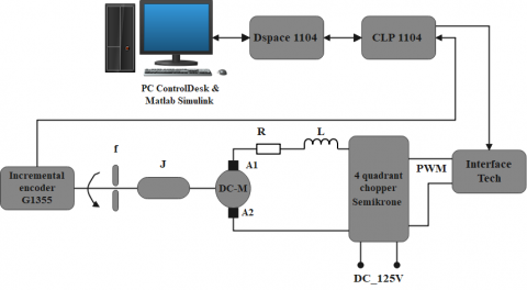
To implement the sliding mode control, the combination between Matlab Simulink to build the SMC control and ControlDesk to control the Dspace 1104 is used. The Dspace 1104 board generates a PWM signal to control the 4-quadrant chopper that will drive the DC motor the feedback is done by the incremental encode (GI355), Figure 11 represents the implementation diagram used.
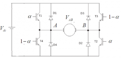
DC motor is excited by its stator at a fixed voltage 125 V and supplied by its rotor by variable voltage via the 4-quadrant chopper, isolation is assured by Tech isolator that also prevents the closing of T1 and T2 or T3 and T4 at the same time then it secures the circuit against short circuits, Figure 12 represents the electrical circuit used to drive the DC motor.
Figure 11. Implementation sliding mode control diagram on DCM
Figure 12. Four quadrant chopper drive DC motor
To deduce α the duty cycle to control the switches T1,2,3,4 it is necessary to calculate the voltage VAB.
${{V}_{A}}=\alpha {{V}_{dc}}$ and ${{V}_{B}}=\left( 1-\alpha \right){{V}_{dc}}$ (21)
As result,
${{V}_{AB}}=\left( 2\alpha -1 \right){{V}_{dc}}{{_{{}}}_{{}}}s{{o}_{{}}}_{{}}\alpha =\frac{1}{2}\left( \frac{{{V}_{AB}}}{{{V}_{dc}}}+1 \right)$ (22)
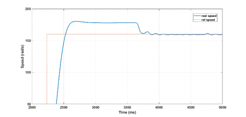
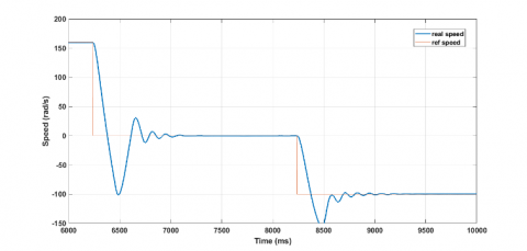
Figure 13. DCM speed response
Figure 13 shows that DCM speed follows the reference speed perfectly with a very short response time, the speed response is satisfactory in both directions of rotation, but the overshot changes according to the speed of rotation, because using the same sliding mode gain kg for all speeds. chattering effect causes legible oscillation shown in DCM speed response close-up view Figure 14.
Figure 14. DCM speed response close-up view
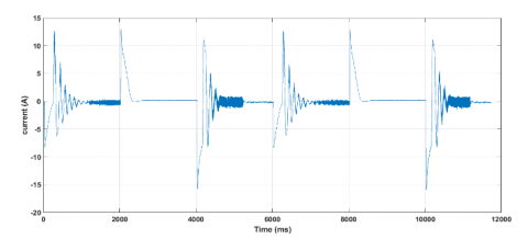
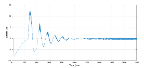
Figure 15. DCM current response
Figure 16. DCM current response close-up view
Figure 15 shows that DCM develops a current for each speed demand that causes speed short response time, the current also changes direction depending on the direction of rotation, the same remark for the overshot changes according to the current that the machine developed, because using the same sliding mode gain Kg. chattering effect causes legible oscillation is shown in DCM current response close-up view Figure 16, theoretically [6-8] the more you increase the value of Kg the smaller the response time (it takes 500 ms for the speed to return to normal Figure 14) will be but the more this oscillation effect increases.
In this paper, sliding mode Control for DC Motor systems with Dead-Zone has been exposed, the dead zone presents the non-linearity caused by Coulomb friction torque, the DC motor is driven by a four-quadrant chopper.
From the simulation and implementation results obtained, it can be said that the sliding mode control brings high robustness against non-linearity and identification uncertainty.
|
Ra |
Armature resistance Ω |
|
La |
Armature resistance Henry |
|
Za |
Armature impedance Ω |
|
fv |
Viscous friction N.m/rad/s |
|
J |
Total moment Inertia kg.m2 |
|
K |
EMF constant |
|
τmec |
Mechanical Time constant |
|
Cc |
Coulomb friction torque |
|
kgs |
Speed sliding mode constant |
|
kgc |
current sliding mode constant |
|
Cf |
viscous friction torque |
|
CEMF |
EMF torque |
[1] Rao, C., Sukumar, G. (2018). Design and analysis of torque ripple reduction in brushless dc motor using SPWM and SVPWM with pi control. European Journal of Electrical Engineering, 20(1): 7-22. https://doi.org/10.3166/ejee.20.7-22
[2] Fezazi, O., Haddj El Mrabet, A., Belkraouane, I., Attou, A. (2021). Nonlinear identification and modeling of a DC motor for bidirectional operation. 1st International Conference on Sustainable Energy and Advanced Materials, IC-SEAM’21 April 21-22, Ouargla, Algeria.
[3] Virgala, I., Frankovský, P., Kenderová, M. (2013). Friction effect analysis of a DC motor. American Journal of Mechanical Engineering, 1(1): 1-5.
[4] Zheng, F., Wang, Q.G., Lee, T.H., Huang, X. (2001). Robust PI controller design for nonlinear systems via fuzzy modeling approach. IEEE Transactions on Systems, Man, and Cybernetics-Part A: Systems and Humans, 31(6): 666-675. https://doi.org/10.1109/3468.983422
[5] Shyam, A., JL, F.D. (2013). A comparative study on the speed response of BLDC motor using conventional PI controller, anti-windup PI controller and fuzzy controller. In 2013 International Conference on Control Communication and Computing (ICCC), Thiruvananthapuram, India, pp. 68-73. https://doi.org/10.1109/ICCC.2013.6731626
[6] Slotine, J., Li, E. (1998). Applied Nonlinear Control. Prence Hall, USA
[7] Oukaci, A., Toufouti, R., Dib, D., Atarsia, L. (2017). Comparison performance between sliding mode control and nonlinear control, application to induction motor. Electrical Engineering, 99(1): 33-45. https://doi.org/10.1007/s00202-016-0376-3
[8] Mobayen, S. (2015). An adaptive chattering-free PID sliding mode control based on dynamic sliding manifolds for a class of uncertain nonlinear systems. Nonlinear Dynamics, 82(1): 53-60. https://doi.org/10.1007/s11071-015-2137-7
[9] Slotine, J. (1984). Sliding controller design for nonlinear Systems. IGC, 40(2): 421-434.
[10] Báez, E., Bravo, Y., Leica, P., Chávez, D., Camacho, O. (2017). Dynamical sliding mode control for nonlinear systems with variable delay. In 2017 IEEE 3rd Colombian Conference on Automatic Control (CCAC), Cartagena, Colombia, pp. 1-6. https://doi.org/10.1109/CCAC.2017.8276426
[11] Chen, Y., Wei, Y., Zhong, H., Wang, Y. (2016). Sliding mode control with a second-order switching law for a class of nonlinear fractional order systems. Nonlinear Dynamics, 85(1): 633-643. https://doi.org/10.1007/s11071-016-2712-6
[12] Jang, J.O., Jeon, G.J. (2000). A parallel neuro-controller for DC motors containing nonlinear friction. Neurocomputing, 30(1-4): 233-248. https://doi.org/10.1016/S0925-2312(99)00128-9
[13] Kara, T., Eker, I. (2004). Nonlinear modeling and identification of a DC motor for bidirectional operation with real time experiments. Energy Conversion and Management, 45(7-8): 1087-1106. https://doi.org/10.1016/j.enconman.2003.08.005
[14] Slotine, J.J., Coetsee, J.A. (1986). Adaptive sliding controller synthesis for non-linear systems. International Journal of Control, 43(6): 1631-1651. https://doi.org/10.1080/00207178608933564
[15] Khalil, H.K. (2002). Nonlinear systems. NJ, USA Prentice Hall.
[16] Nordin, M., Gutman, P.O. (2002). Controlling mechanical systems with backlash—A survey. Automatica, 38(10): 1633-1649. https://doi.org/10.1016/S0005-1098(02)00047-X
[17] Buhler, H. (1986). Control by sliding mode. Presses Polytechnic Romandes, Lausanne.
[18] Utkin, V., Guldner, J., Shi, J. (1999). Sliding Mode Control in Electromechanical System. Taylor & Francis, London.
[19] Hadda, B., Larbi, C.A., Abdessalam, M. (2018). A new technique of second order sliding mode control applied to induction motor. European Journal of Electrical Engineering, 20(4): 399.