Said Amrane* | Abdallah Zahidi | Mostafa Abouricha | Nawfel Azami | Naoual Nasser | Mohamed Errai
© 2021 IIETA. This article is published by IIETA and is licensed under the CC BY 4.0 license (http://creativecommons.org/licenses/by/4.0/).
OPEN ACCESS
Solenoid valves represent indispensable elements in various engineering systems. Their failure can lead to unexpected problems. This failure may be caused by fluctuations in the coil resistance of the electromagnetic solenoid (EMS) which actuates these solenoid valves. Hence the need to monitor this parameter for a preventive maintenance of these actuators. The proposed method consists to use supervised machine learning to monitor coil resistance of the EMS valve. The EMS valve is coupled to an optical fiber squeezer which, acts as a force sensor. The solenoid armature applies a mechanical force to the optical fiber and changes the polarization state of the light that travels through the optical fiber and then this force infects the power of the light. A Simulink model is used to determine the open loop system step response. The identification of the system allows obtaining its transfer function, which depends on the parameters of the EMS and in particular on its coil resistance. By varying the coil resistance while fixing the other physical parameters of the EMS, we generate a database whose elements are the coefficients of the transfer function of the solenoid open loop and the electrical resistance of its coil. The generated database is used for training several supervised machine learning models whose predictors are the elements of the transfer function; the response is the coil resistance. The Gaussian process for regression allows to predict the variations of the coil resistance with the smallest relative error although it takes a relatively long time for the training compared to the other models used.
machine learning, monitoring, solenoid valve, coil resistance, fiber squeezer
Electromechanical solenoids (EMS) have relatively an inexpensive conception [1], their control circuit and design are simple. They are very reliable and require low power for control [2]. They are used in a wide range of modern industrial equipment such as digital actuator arrays [3], gas valve [4], robotic manipulators [5], positioners [6], anti-braking systems [7], vehicle vibration control systems [8], and polarization controllers where they are used as a mechanical actuator to adjust the light power at the output of an optical fiber [9]. To improve the security measures and performance of the systems based on the EMS, a strategy of regular maintenance of these EMS certainly reduces the failure rate [10]. These failures can be caused by the wear of the contact surfaces of the friction assemblies or/and by the fluctuations of its parameters [11, 12] namely the mass of the armature, the stiffness of the spring, the coefficient of friction, the inductance of the coil and its electrical resistance [13, 14]. Other studies have shown that EMS failure can occur gradually due to the exhaustion of the coil in relation to voltage and mains frequency, and spring stiffness [15, 16]. These EMS failures can lead to serious accidents in the economy and in the safety field such as railway braking system, nuclear power plants and aviation engine [17]. Studies based on signal processing and machine learning were used to develop a sensor to detect anomalies [18, 19] or a method of grouping EMS failures [20] without giving a physical explanation of the failure modes related to the EMS parameters [21]. In one of our previous studies [14], we used a method of monitoring EMS parameters based on an optical fiber squeezer coupled to an artificial neural network (ANN). In this study, we propose to use supervised machine learning to monitor fluctuations in the coil resistance of the EMS. The predictors are the coefficients of the EMS transfer function while the response is its coil resistance. The database used for the training of the machine-learning model is generated from a Simulink model by varying the coil resistance of the EMS, and each time, the transfer function is determined by identification of the dynamic open-loop step response of the EMS. Different regression models are used to predict fluctuations in coil resistance: linear regression (LR) [22], support vector machines for regression (SVM) [23], gaussian process regression (GPR) [24], regression trees (RT) [25], and ensembles of tree (RTE) [26]. the GPR model presents advantages in terms of root mean square error (RMSE) and relative error on the prediction of the variations of the resistance of the coil although it requires a relatively long time for the learning. the SVM model is disadvantageous in terms of RMSE and learning time.
2.1 Structure of the EMS based on fiber squeezer
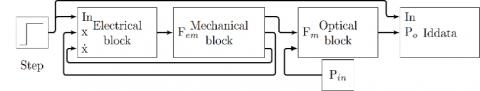
The EMS based on fiber squeezer (Figure 1) consists of an EMS coupled with an optical force sensor [14].
Figure 1. Structure of the EMS with fiber squeezer
A birefringence is created by applying a force to the optical fiber. This birefringence affects the polarization of the light that propagates through the optical fiber [9]. The force is then measured by analyzing the light power at the output of the optical fiber detected by the photodiode.
2.2 Mathematical modeling of the EMS with fiber squeezer
The EMS based on fiber squeezer is subdivided into three sub-blocks, a mechanical block, an electrical block and an optical block. The differential Eq. (1) models the mechanical part of the EMS [27]:
$\frac{d^{2} x}{d t^{2}}=\frac{1}{m}\left(F_{e m}-K\left(x-x_{0}\right)-B \frac{d x}{d t}\right)$ (1)
where, x is the armature displacement, x0 is the initial air gap between the armature and the frame backside, m is the armature mass, K is the spring stiffness, Fem is the electromagnetic force created by the solenoid coil, and B is the coefficient of the system. The electrical block is modeled by the differential Eq. (2):
$U=R i(t)+L(x) \frac{d i(t)}{d t}+i(t) \frac{d L(x)}{d t}$ (2)
where, U is the electrical voltage across the EMS coil, R is the electrical coil resistance of EMS, i(t) is the electromagnetic coil current, and L is the coil inductance of the EMS. The differential Eq. (3) interprets the comportment of the EMS optical block [14]:
$P_{o}=\frac{P_{i}}{2}(1+\cos \delta)$ (3)
where, Pi is the input light power of the optical fiber, P0 is the output light power of the optical and δ is the phase difference between two polarized lights along the squeezing axis and its orthogonal axis that can be expressed as [28]:
$\delta=6.10^{-5} \frac{F}{\lambda d}$ (4)
where, F is the intensity of squeezing force, λ is the wavelength of the used light and d is the diameter of the used optical fiber core.
2.3 Simulink model of the EMS based on fiber squeezer
The Simulink model of the EMS fiber squeezer consists of three interconnected sub-blocks, the mechanical sub-block, the electrical sub-block and the optical sub-block (Figure 2). The mechanical sub-block and the electrical sub-block model respectively the two differential Eqns. (1) and (2) while the optical sub-block models the two Eqns. (3) and (4). The electromagnetic force generated by the coil represents an entry of the mechanical sub-block. The position and the velocity of the armature calculated by the mechanical sub-block constitute a feedback to the electrical sub-block. The optical sub-block is interconnected to the mechanical sub-block via the squeezing force.
Figure 2. Scheme of Simulink model of the EMS based on fiber squeezer
2.4 Estimation of the open loop transfer function
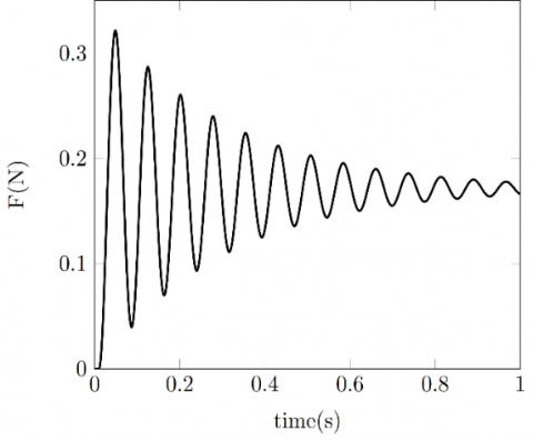
The Simulink model is simulated with the following parameters values: The coil resistance R=10Ω, the inductance L=20mH, the spring stiffness constant K=2000N/m, the friction coefficient B=2Ns/m, and the mass plunger m=300g. The open-loop step response of the system (Figure 3) shows that the system is stable with a damped pseudo-periodic regime.
Figure 3. Open loop step response
The open loop step response is used to estimate the system transfer function using “tfest” function which, is a function integrated in Matlab [29]. The transfer function obtained is expressed in the following form:
$T f=\frac{\text { num }}{s^{2}+\operatorname{den} 2 s+\operatorname{den} 3}$ (5)
where, num is the numerator of the transfer function (in rad2.A2.s-2), den2 (in rad.s-1) and den3 (in rad2.s-2) are the coefficients of the numerator polynomial of the transfer function. For the EMS parameter values indicated in section 2.4. The estimated transfer function is:
$T f=\frac{231.3}{s^{2}+6.857 s+6759}$ (6)
The estimate of the transfer function is established with the following performances: The fit percent of the estimation is 99,39% and the MSE is 1,76.10-7.
2.5 Variation of the coil resistance and creation of the database
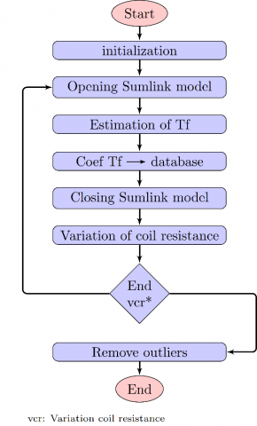
The EMS parameters are fixed to the values indicated in section 2.4. However, we vary the coil resistance from 10 to 50Ω and each time, the Simulink model is executed to obtain the step response of the open loop system. Then the system is identified using the tfest function to determine the coefficients of the system transfer function. The coil resistance of the EMS and those of the transfer function are saved in a database which, has four columns (R, num, den2 and den3) and 10000 rows. Finally, a preprocessing of this database is executed to remove the outliers. The flowchart presented in the Figure 4 summarizes the different steps followed to create this database.
Figure 4. Flowchart of database generation
2.6 The effect of varying the coil resistance on the transfer function parameters
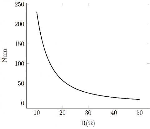
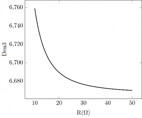
The transfer function coefficients depend on the EMS parameters [14]. In particular, the variation of the coil resistance varies the system transfer function. The following figures (Figure 5(a) to Figure 5(c)) represent the variation of the transfer function coefficients as a function of the coil resistance. Note that all the transfer function coefficients decrease when the coil resistance increases.
(a)
(b)
(c)
Figure 5. (a) Variation of num as function of R; (b) Variation of den2 as function of R; (c) Variation of den3 as function of R
3.1 Machine learning training
We propose to use the supervised machine learning to predict the coil resistance value from the open loop step response of the EMS. The regression learner toolbox integrated in the Matlab environment can performs this kind of task. With this toolbox, we can use different models of regression: linear regression (LR) [22], support vector machines for regression (SVM) [23], gaussian process regression (GPR) [24], regression trees (RT) [25], and ensembles of tree (RTE) [26]. In our case, the predictors are the transfer function parameters (num, den2, and den3) and the response is the coil resistance (R). Table 1 summarizes the performances of these different models.
Table 1. Performance of the used different regression methods
|
|
SVM |
LR |
RT |
RTE |
GPR |
|
R-squared |
0.99 |
1 |
1 |
1 |
1 |
|
RMSE |
1.06 |
0.10 |
0.09 |
0.02 |
0.00 |
3.2 Prediction of coil resistance & testing of ml models performance
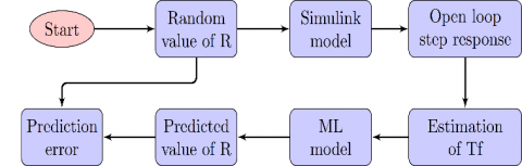
To predict the coil resistance value, it is sufficient to run the Simulink model (R is unknown) to determine its open loop step response. The coefficients transfer function of the EMS are determined using the tfest function. These coefficients are injected into the machine-learning model to find the coil resistance value at the exit of the model.
The flowchart presented in the Figure 6 summarizes the different steps followed to predict the coil resistance and the relative error on this prediction.
Figure 6. Flowchart of coil resistance prediction
Table 2. Relative error of the used different regression methods
|
|
Test 1 |
Test 2 |
Test 3 |
|
R |
16.79Ω |
29.80Ω |
33.60Ω |
|
SVM |
0.2864% |
1.2900% |
2.5528% |
|
LR |
7.6946% |
4.5220% |
3.7306% |
|
RT |
0.4670% |
0.1477% |
0.0115% |
|
RTE |
0.0275% |
0.0777% |
0.0528% |
|
GPR |
0.0085% |
0.0302% |
0.0379% |
The figures Figure 5(a) to Figure 5(c) show that the three transfer function coefficients of the EMS strongly depend on the coil resistance. Each of these coefficients decreases when the coil resistance increases. The machine learning models used allow to predict the coil resistance of the EMS with differences in precision and training time. The training time is relatively long for the SVM and the GRP models. Table 1 shows that all the methods have a good R-squared coefficient (about 1), which, implies that there is a good correlation between the coil resistance and the transfer function coefficients [30]. The RMSE coefficient varies depending on the model used. So RT, RTE, and GPR have good performance (RMSE close to 0), which implies that the predicted values are close to the real values. The Table 2 represent the relative error of the prediction on the coil resistance. Note that the prediction quality is good for the RT, RTE, and GPR methods. But the GRP method has the lowest relative error (less than 0,03%).
In this work, an approach is proposed to detect fluctuations in the coil resistance of an EMS valve. A Simulink model of the EMS valve is used to determine the dynamic open-loop step response. This response depends on the physical parameters of the EMS. A database is generated by varying the coil resistance of the EMS valve while keeping the other parameters fixed. This database is used for training various supervised machine-learning models. The models used are the linear regression (LR), the regression tree (RT), the regression tree ensemble (RTE), the support machine vector for regression (SVM) and the Gaussian process for regression (GPR). The models used have different performance in terms of training time and the root mean square error (RMSE). The GPR model takes a relatively long time to train, but it allows to predict the coil resistance of the EMS valve with the smallest relative error (less than 0.03%).
In the future work, another study is envisaged for the monitoring of all physical parameters of EMS valve using the supervised machine learning.
[1] Yu, L., Chang, T.N. (2007). Zero vibration on-off position control of dual solenoid actuator. In IECON 2007 - 33rd Annual Conference of the IEEE Industrial Electronics Society, pp. 775-780. https://doi.org/10.1109/TIE.2009.2036031
[2] Bochkarev, I.V., Bryakin, I.V., Khramshin, V.R. (2018). Control of operational condition of electromagnetic devices of automation systems. In 2018 International Conference on Industrial Engineering, Applications and Manufacturing (ICIEAM), pp. 1-6. https://doi.org/10.1109/ICIEAM.2018.8728640
[3] Petit, L., Hassine, A., Terrien, J., Lamarque, F., Prelle, C. (2014). Development of a control module for a digital electromagnetic actuators array. IEEE Transactions on Industrial Electronics, 61(9): 4788-4796. https://doi.org/10.1109/TIE.2013.2290755
[4] Sosa, A., Bollinger, D.S., Karns, P.R. (2017). Performance characterization of a solenoid-type gas valve for the H- magnetron source at FNAL. In AIP Conference Proceedings, 1869(1): 020014. https://doi.org/10.1063/1.4995720
[5] Takai, A., Alanizi, N., Kiguchi, K., Nanayakkara,T. (2013). Prototyping the flexible solenoid-coil artificial muscle, for exoskeletal robots. In 2013 13th International Conference on Control, Automation and Systems (ICCAS 2013), pp. 1046-1051. https://doi.org/10.1109/ICCAS.2013.6704071
[6] Chen, M.Y., Huang, H.H., Hung, S.K. (2010). A new design of a submicropositioner utilizing electromagnetic actuators and flexure mechanism. IEEE Trans. Ind. Electron., 57: 96-106. https://doi.org/10.1109/TIE.2009.2033091
[7] Chu, L., Hou, Y., Liu, M., Li, J., Gao, Y., Ehsani, M. (2007). Study on the dynamic characteristics of pneumatic ABS solenoid valve for commercial vehicle. In 2007 IEEE Vehicle Power and Propulsion Conference, pp. 641-644. https://doi.org/10.1109/VPPC.2007.4544201
[8] Koch, U., Wiedemann, D., Ulbrich, H. (2011). Model-based MIMO state-space control of a car vibration test rig with four electromagnetic actuators for the tracking of road measurements. IEEE Transactions on Industrial Electronics, 58(12): 5319-5323. https://doi.org/10.1109/TIE.2010.2044740
[9] Rumbaugh, S.H., Jones, M.D., Casperson, L.W. (1990). Polarization control for coherent fiber-optic systems using nematic liquid crystals. Journal of Lightwave Technology, 8(3): 459-465. https://doi.org/10.1109/50.50741
[10] Tang, X., Peng, J., Chen, B., Jiang, F., Yang, Y., Zhang, R., Gao, D., Zhang, X. (2019). A parameter adaptive data-driven approach for remaining useful life prediction of solenoid valves. 2019 IEEE International Conference on Prognostics and Health Management (ICPHM), pp. 1-6. https://doi.org/10.1109/ICPHM.2019.8819382
[11] Cvetkovic, D., Cosic, I., Subic, A. (2008). Improved performance of the electromagnetic fuel injector solenoid actuator using a modelling approach. International Journal of Applied Electromagnetics and Mechanics, 27(4): 251-273. https://doi.org/10.3233/JAE-2008-939.
[12] Kabib, M., Batan, I.M.L., Pramujati, B., Sigit, A.S.I. (2006). Modelling and simulation analysis of solenoid valve for spring constant influence to dynamic response. Transfer, 2(1): 10.
[13] Lunge, S.P., Kurode, S.R., Chhibber, B. (2013). Proportional actuator from on off solenoid valve using sliding modes. In Proceedings of the 1st International and 16th National Conference on Machines and Mechanisms (iNaCoMM2013), pp. 1020-1027.
[14] Zahidi, A., Said, A., Azami, N., Nasser, N. (2020). Effect of fiber and solenoid variation parameters on the elements of a corrector PID for electromagnetic fiber squeezer based polarization controller. International Journal of Electrical and Computer Engineering, 10(3): 2441. https://doi.org/10.11591/ijece.v10i3
[15] Liniger, J., Stubkier, S., Soltani, M., Pedersen, H.C. (2020). Early detection of coil failure in solenoid valves. IEEE/ASME Transactions on Mechatronics, 25(2): 683-693. https://doi.org/10.1109/TMECH.2020.2970231
[16] Mercer, J.R. (1969). Paper 12: Reliability of solenoid valves. In Proceedings of the Institution of Mechanical Engineers, Conference Proceedings, 184(2): 89-94. https://doi.org/10.1243/PIME_CONF_1969_184_044_02
[17] Tang, X., Xiao, M., Liang, Y., Hu, B., Zhang, L. (2018). Application of particle filter technique to online prognostics for solenoid valve. Journal of Intelligent & Fuzzy Systems, 35(1): 523-532. https://doi.org/10.3233/JIFS-169608
[18] Perotti, J.M. (2010). KEA-71 Smart Current Signature Sensor (SCSS). NASA Tech Report n°20110000497.
[19] Perotti, J.M., Lucena, A., Ihlefeld, C., Burns, B., Bassignani, M. (2005). Washington, DC: U.S. Patent and Trademark Office. U.S. Patent No. 6,917,203.
[20] Tsai, H.H., Tseng, C.Y. (2010). Detecting solenoid valve deterioration in in-use electronic diesel fuel injection control systems. Sensors, 10: 7157-7169. https://doi.org/10.3390/s100807157
[21] Tod, G., Mazaev, T., Eryilmaz, K., Ompusunggu, A., Hostens, E., Hoecke, S. (2019). A convolutional neural network aided physical model improvement for AC solenoid valves diagnosis. 2019 Prognostics and System Health Management Conference (PHM-Paris), pp. 223-227. https://doi.org/10.1109/PHM-Paris.2019.00044
[22] Kavitha, S., Varuna, S., Ramya, R. (2016). A comparative analysis on linear regression and support vector regression. 2016 Online International Conference on Green Engineering and Technologies (IC-GET), pp. 1-5. https://doi.org/10.1109/GET.2016.7916627
[23] Smola, A.J., Schölkopf, B. (2004). A tutorial on support vector regression. Statistics and Computing, 14(3): 199-222. https://doi.org/10.1023/B:STCO.0000035301.49549.88
[24] Quinonero-Candela, J., Rasmussen, C.E. (2005). A unifying view of sparse approximate Gaussian process regression. The Journal of Machine Learning Research, 6: 1939-1959.
[25] Loh, W.Y. (2011). Classification and regression trees. Wiley Interdisciplinary Reviews: Data Mining and Knowledge Discovery, 1(1): 14-23. https://doi.org/10.1002/widm.8
[26] Linero, A.R., Yang, Y. (2018). Bayesian regression tree ensembles that adapt to smoothness and sparsity. Journal of the Royal Statistical Society: Series B (Statistical Methodology), 80(5): 1087-1110. https://doi.org/10.1111/rssb.12293
[27] Dong, D., Li, X. (2012). Simulation and experimental research on the response of a novel high-pressure pneumatic pilot-operated solenoid valve. In 2012 19th International Conference on Mechatronics and Machine Vision in Practice (M2VIP), pp. 480-484.
[28] Smith, A.M. (1980). Single-mode fibre pressure sensitivity. Electronics Letters, 16(20): 773-774. https://doi.org/10.1049/el:19800548
[29] Najdek, K., Nalepa, R., Zygmanowski, M. (2019). Identification of Dual-Active-Bridge converter transfer function. Przegląd Elektrotechniczny, 3: 151-154. https://doi.org/10.15199/48.2019.03.33
[30] Cameron, A.C., Windmeijer, F.A. (1997). An R-squared measure of goodness of fit for some common nonlinear regression models. Journal of Econometrics, 77(2): 329-342. https://doi.org/10.1016/S0304-4076(96)01818-0