Mukul Kumar Gupta* | Roushan Kumar | Varnita Verma | Abhinav Sharma
© 2021 IIETA. This article is published by IIETA and is licensed under the CC BY 4.0 license (http://creativecommons.org/licenses/by/4.0/).
OPEN ACCESS
In this paper the stability and tracking control for robot manipulator subjected to known parameters is proposed using robust control technique. The modelling of robot manipulator is obtained using Euler- Lagrange technique. Three link manipulators have been taken for the study of robust control techniques. Lyapunov based approach is used for stability analysis of triple link robot manipulator. The Ultimate upper bound parameter (UUBP) is estimated by the worst-case uncertainties subject to bounded conditions. The proposed robust control is also compared with computer torque control to show the superiority of the proposed control law.
triple link manipulator, Euler Lagrange, robust control, Lyapunov analysis
Robot manipulator system has many subsystems like drive system, manipulator arm, sensors and controllers. Some of the controller design concern in case robot design are like drive system (hydraulic, pneumatic and electromagnetic) used in robotics so the factors affecting control solution are robustness, nonlinearities, disturbances, unmodelled dynamics, torque ripples, stability problem, load disturbances and noise. In case of sensor system factors affecting control, solution is multisensory environment, controller design, signal processing and sensor programing etc. Other concern with structure like limped or distributed mass with inertia effect, actuator failure, speed constraint, degree of freedom, external factor etc. There are many control approaches like PID control [1], state feedback control, sliding, robust and adaptive control, Intelligent (Fuzzy and Neural) Control [2-8], LQR Control and optimal control [9]. As even single link manipulator is nonlinear in nature so conventional control technique is not suitable for the control of multilink manipulator as nonlinearities increasing in a drastic manner [10]. In past years, many robust control techniques have been proposed to overcome nonlinearities and disturbances for control of robot manipulator [11-15].
A proper uncertainty bound parameter is preferred in order to improve the performance of robust control system. The estimation of uncertainty bound parameters is taken carefully in order to obtain optimum solutions. Estimating too high upper bound parameter can cause higher chattering frequency, input saturation etc. Many of the presented techniques in the past are very complex in nature and contains too much complexity [16-18]. As we know multilink robot manipulator are having many applications either in defense, aerospace or in industrial automation. In order to obtain tracking of desired trajectories, the control problems need to be solved efficiently using proper control system technique. As in robust control wide range of uncertainties are considered which is a result of ultimate upper bound of tracking error stability analysis using Lyapunov method.
The control of robot manipulators for better stability analysis has become an applied research area among research scholars. The most common drawback of the control techniques being used in the majority of the problems is the negligence of the nonlinear effects of the robotic systems. Another drawback is the negligence of time delays. In dynamical systems, the performance and stability of the systems is highly influenced by time delays. This has also been an extensive research topic for many years. As manipulator is highly nonlinear in nature so control of manipulator is very challenging when all the nonlinearities are considered. Slotine et al. [19-21] focuses on the uncertainty bound parameter (UBP) to design the robust control of electrical manipulators. The UBP is commonly obtained by considering the worst case of uncertainties in bounding functions. However, too high estimation of UBP may cause saturation of input, higher frequency of chattering in the switching control laws, and thus a bad behavior of the whole system, while too low estimation of UBP may cause a higher tracking error. Tao [22] addresses the problem of the accurate task space control subject to finite-time convergence. In the article design of adaptive-robust finite-time nonlinear control inputs for uncertain robot manipulators global finite stability for robot manipulator considered [23, 24]. Robust and Computed Torque Control (CTC) trajectory tracking objective is studied for a wide group of degrees of freedom (DOF) robot manipulators subjected to parametric and modeling uncertainties. Inspired by the aforementioned discussions, in this paper a simplified and modern robust control law is proposed for Euler- LaGrange system is subjected to known parameters. Also, comparison in robust and CTC technique has been discussed and superiority of the robust control easily be seen from the obtained result. The paper is organized as follows. In section II stability analysis of manipulator is discussed. In section III triple link manipulator system is considered followed by application and various result of trajectory tracking and tracking error in section IV respectively.
In general, the dynamics of manipulator can be written as:
$M\ddot{q}+C\dot{q}+G=\tau $ (1)
where, $q \in \mathbb{R}^{n}$ is state of the system, $\tau \in \mathbb{R}^{n}$ is the control inut, $M \in \mathbb{R}^{n x n}$ is the mass or inertia matrix, C$\in \mathbb{R}^{n x n}$ denoted the Coriolis or centripetal terms, $G \in \mathbb{R}^{n}$ denotes the gravitational force. The manipulator dynamics is denoted as:
$m\ddot{q}+mgl\sin (q)=\tau $ (2)
Assumption 1: The desired trajectory $q_{d}(t)$ is designed in a manner such that $q_{d}, \dot{q}_{d}, \ddot{q}_{d} \in L_{\infty}$. When mass m and length l are known constants. Objective tracking control – The difference between desired trajectory $q_{d}(t)$ and given trajectory $q(t)$ is error dynamics $(e)$. for designing of a tracking controller error dynamics $e \rightarrow 0$ as $t \rightarrow 0$. The error dynamics $e=q_{d}(t)-q(t)$ and derivative of error dynamics is:
$\dot{e}={{\dot{q}}_{d}}(t)-\dot{q}(t)$ (3)
Control input still does not appear in rate of change of error dynamics so from EL dynamics:
$\ddot{e}={{\ddot{q}}_{d}}(t)-\ddot{q}(t)$ (4)
Now as per dynamics of the system $\ddot{q}=-g l \sin (q)+\tau / m$, clearly control input appear in $\ddot{q}$. Lyapunov approach is most widely used method as in this approach without solving the equations stability can be analyzed. For Stability analysis a positive Lyapunov Function $V$ selected and adjust a controller to achieve $\dot{V}(e)$ is Negative definite (N.D.) / Negative semi definite (N.S.D.).
2.1 Robust control
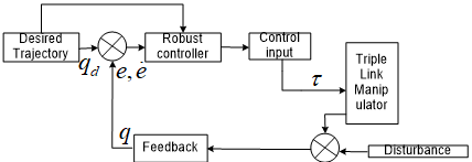
The manipulator system in general, represent a large class of real-world problem like Backhoe, Lower and upper limb Exoskeleton, Aircraft, Biomechanics, Manipulator, Wheeled and mobile robots etc. These systems have various application in many domains such as automation, spacecraft, surveillance Medical etc. In this paper Robust control technique has been propound for tracking control of manipulator systems and Lyapunov based stability analysis also discussed to show the effectiveness of the controller [14]. The main advantage of the controller is that it is very easy to implement. Moreover, the proposed robust controller is validated on triple link manipulator. The basic control structure of robust control is shown in Figure 1 in which $v_{R}$ is used to deal with disturbances and noise. In the given diagram, feedback terms make sure system is closed loop and stable. Robust term takes care of noise and disturbances. The control law consists of both feedback and feedforward term.
From the Figure 1, it is clear that the control law will be $u=-K x+v_{R}$. Let us assume that $v_{R}=-k_{2} x$, so control law become $u=-K x-k_{2} x$.
Figure 1. Closed loop system subjected to noise and disturbances
2.2 Stability analysis
The following Lyapunov function has been assumed for stability analysis of proposed system.
$V(r)=\frac{1}{2}m{{r}^{2}}$ (5)
where,
$r=\dot{e}+\beta e$ (6)
seeking $\dot{V}(r)=-k r^{2}$, Filter tracking error- $r=\dot{e}+\beta e$, where β is positive constant (can be considered as control gain).
Lemma: if $r \in L_{\infty} \& r \rightarrow 0$ as $t \rightarrow \infty$, then $e, \dot{e} \rightarrow 0$.
Proof – if $r \in L_{\infty}$ implies $|r|<\epsilon$ substituting in to $r=\dot{e}+\beta$ e yields $|\dot{e}+\beta e|<\varepsilon$ which can further bounded as$|\dot{e}+\beta e|<\varepsilon$ or $|\dot{e}|<\beta|e|+\varepsilon$, solve for the inequality obtains $|e(t)<C| e(0) e^{-\beta t}+\frac{\varepsilon}{\beta}\left(1+e^{-\beta t}\right)$ means $|e(t)|<0$ as $\epsilon \rightarrow 0$ and as $t \rightarrow \infty$.( QED).
Properties 1: if r $\in L_{\infty} \text { then } e, \dot{e} \in L_{\infty}$.
Properties 2: if r $r \in L_{2}$ then $e, \dot{e} \in L_{2}$.
Properties 3: if $r \rightarrow 0$ then $e, \dot{e} \rightarrow 0$.
Let us define the error dynamics $r=\dot{e}+\beta e$, where $\beta$ is the tracking error of robot defined as $e=q_{d}(t)-q(t)$. Consider the following function which is positive definite $V(r)=\frac{1}{2} m r^{2}$.
Taking the time derivative of Eq. (5), $\dot{V}(r)=r m \dot{r}$ put the value of $r=\dot{e}+\beta e$ then,
$\dot{V}(r)=rm(\ddot{e}+\beta \dot{e})$ (7)
From $\ddot{e}=\ddot{q}_{d}(t)-\ddot{q}(t)$, substitute the value of $\ddot{q}(t)$.
$\dot{V}(r)=rm({{\ddot{q}}_{d}}(t)-(-gl\sin (q)+\tau /m)+\beta \dot{e})$ (8)
As per Lyapunov theorem, $\dot{V}(r)$ should be negative definite so control input $\tau$ has to be selected such that,
$\tau =m({{\ddot{q}}_{d}}(t)+gl\sin (q)+\beta \dot{e}+kr)$ (9)
Now $\dot{V}(r)=-k r^{2}$, which is negative definitive, proves the stability of the system.
For worst case analysis let us consider torque as $\tau=K r+v_{R}$, where Kr is a feedback term and $v_{R}$ is disturbances present in the system. Time derivative of Eq. (6)
$\dot{r}=\ddot{e}+\beta e$ (10)
Put the value of $\dot{r}$ from Eq. (10), we get:
$m \dot{r}=m(\ddot{e}+\beta e)=m\left\{\left(\ddot{q}_{d}-\ddot{q}\right)+\beta e\right\}$
$m r=m \ddot{q}_{d}+m g l \sin (q)+\beta m \dot{e}-\tau$ (11)
Choose the Lyapunov function candidate as:
$V(e,r)=\frac{1}{2}m{{r}^{2}}+\frac{1}{2}{{\beta }^{2}}m{{e}^{2}}$ (12)
Time derivative of Eq. (12).
$\dot{V}(e,r)=rm\dot{r}+{{\beta }^{2}}me\dot{e}$ (13)
$\dot{V}(e,r)=rm({{\ddot{q}}_{d}}-\ddot{q}+\beta \dot{e})+{{\beta }^{2}}me\dot{e}$ (14)
Substitute the value of $\ddot{q}$ from Eq. (2) and rearranging the terms such that $\dot{V}$ become negative definite,
$\dot{V}(e, r)=r\left[m \ddot{q}_{d}+m g l \sin (q)+\beta m \dot{e}-\tau\right]$
$+\beta^{2} m e \dot{e}$
$\dot{V}(e, r)=r\left[m \ddot{q}_{d}+m g l \sin (q)+\beta m(r-\beta e)-\tau\right]$
$+\beta^{2} m e(r-\beta e)$
$\dot{V}(e, r)=r\left[m \ddot{q}_{d}+m g l \sin (q)\right]+\beta m r^{2}-\beta^{2} m e r-r\left(K r+v_{R}\right)$
$+\beta^{2} m e r-\beta^{3} m e^{2}$ (15)
Let $r\left(m \ddot{q}_{d}+m g l \sin (q)\right) \leq|r| C_{1}$.
$\dot{V}(e,r)\le |r|{{C}_{1}}-(K-\beta m){{r}^{2}}-r{{v}_{R}}-{{\beta }^{3}}m{{e}^{2}}$ (16)
Eq. (16) will be good term if $K>\beta m$.
Let $K_{2}=K-\beta$m and $v_{R}=K_{3} C_{1}{ }^{2} r$ then,
$\dot{V}(e, r) \leq-K_{2} r^{2}-\beta^{3} m e^{2}+|r| C_{1}-K_{3} C_{1}^{2} r^{2}$
$\dot{V}(e,r)\le -{{K}_{2}}{{r}^{2}}-{{\beta }^{3}}m{{e}^{2}}+\frac{1}{4{{K}_{3}}}$ (17)
using $-a y^{2}+b y+c=-\left(y-\frac{b}{2 a}\right)^{2}+\frac{b^{2}}{4 a^{2}}+c$
$\dot{V}(e, r) \leq-K_{3} C_{1}^{2} r^{2}+|r| C_{1}+\ldots .$
$\dot{V}(e, r) \leq\left(|r|-\frac{C_{1}}{2 K_{3} C_{1}^{2}}\right)^{2}+\frac{C_{1}^{2}}{4 K_{3} C_{1}^{2}}$
$-(K-\beta m) r^{2}-\beta^{3} m e^{2}$
$\dot{V}(e,r)\le \frac{1}{4{{K}_{3}}}-(K-\beta m){{r}^{2}}-{{\beta }^{3}}m{{e}^{2}}$ (18)
$\dot{V}(e, r) \leq-K_{2} r^{2}-\beta^{3} m e^{2}+\frac{1}{4 K_{3}}=0$
$\leq-\min \left(K_{2}, \beta^{3} m\right)\|\mathrm{W}\|+\frac{1}{4 K_{3}}, \mathrm{~W} \triangleq\left[\begin{array}{l}e \\ r\end{array}\right]$ (19)
The value will be:
$\begin{aligned}\|\mathrm{w}\|^{2}=& \frac{1}{4 K_{3} \mathrm{~m} \operatorname{in}\left(K_{2}, \beta^{3} m\right)} \mathrm{or}, \\ &|| W||=\sqrt{\frac{1}{4 K_{3} \min \left(K_{2}, \beta^{3} m\right)}} \end{aligned}$ (20)
From Eq. (20) clearly shows the UUP value of TLP system.
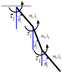
Triple Link Manipulator- The triple link distributed pendulum (TLDP) is taken as part of study as there is not work is available in the literature and also, it’s a very highly nonlinear system for control point of view which shown in Figure 2. The modelling of TLDP is obtained using Euler LaGrange technique where LaGrange is the difference in kinetic energy and potential energy is given in Appendix.
Figure 2. Schematic of triple link manipulator
The detailed dynamics is given by Gupta [10] where Mass matrix $M \in \mathbb{R}^{n x n}$, Coriolis matrix $\mathrm{C} \in \mathbb{R}^{n x n}$ and Gravity matrix $G \in \mathbb{R}^{n}$ term is combined together so that control law can be applied in a suitable manner.
$M(q,\ddot{q})=\left[ \begin{matrix} {{I}_{c1}}+\frac{{{m}_{1}}l_{1}^{2}}{4}+{{m}_{2}}l_{1}^{2}+{{m}_{3}}l_{1}^{2} & \frac{{{m}_{2}}}{2}{{l}_{1}}{{l}_{2}}\cos ({{\theta }_{1}}-{{\theta }_{2}})+{{m}_{3}}{{l}_{1}}{{l}_{2}}\cos ({{\theta }_{1}}-{{\theta }_{2}}) & \frac{{{m}_{3}}}{2}{{l}_{1}}{{l}_{3}}\cos ({{\theta }_{3}}-{{\theta }_{1}}) \\ \frac{{{m}_{2}}}{2}{{l}_{1}}{{l}_{2}}\cos ({{\theta }_{1}}-{{\theta }_{2}})+{{m}_{3}}{{l}_{1}}{{l}_{2}}\cos ({{\theta }_{1}}-{{\theta }_{2}}) & {{I}_{c2}}+\frac{{{m}_{2}}l_{2}^{2}}{4}+{{m}_{3}}l_{2}^{2} & \frac{{{m}_{3}}}{2}{{l}_{2}}{{l}_{3}}\cos ({{\theta }_{2}}-{{\theta }_{3}}) \\ \frac{{{m}_{3}}}{2}{{l}_{1}}{{l}_{3}}\cos ({{\theta }_{3}}-{{\theta }_{1}}) & \frac{{{m}_{3}}}{2}{{l}_{2}}{{l}_{3}}\cos ({{\theta }_{2}}-{{\theta }_{3}}) & {{I}_{c3}}+\frac{{{m}_{3}}l_{3}^{2}}{4}\text{ } \\ \end{matrix} \right]$
$C(q,\dot{q})=\left[ \begin{matrix} 0 & (0.5{{m}_{2}}+{{m}_{3}}){{l}_{1}}{{l}_{2}}\sin ({{\theta }_{1}}-{{\theta }_{2}}) & 0.5{{m}_{3}}{{l}_{1}}{{l}_{3}}\sin ({{\theta }_{1}}-{{\theta }_{3}}) \\ -(0.5{{m}_{2}}+{{m}_{3}}){{l}_{1}}{{l}_{2}}\sin ({{\theta }_{1}}-{{\theta }_{2}}) & 0 & 0.5{{m}_{3}}{{l}_{2}}{{l}_{3}}\sin ({{\theta }_{1}}-{{\theta }_{2}}) \\ -0.5{{m}_{3}}{{l}_{1}}{{l}_{3}}\sin ({{\theta }_{1}}-{{\theta }_{3}}) & 0.5{{m}_{3}}{{l}_{2}}{{l}_{3}}\sin ({{\theta }_{2}}-{{\theta }_{3}}) & 0 \\ \end{matrix} \right]$
$G(q)={{\left[ \begin{matrix} (0.5{{m}_{1}}+{{m}_{2}}+{{m}_{3}})g{{l}_{1}}\sin {{\theta }_{1}} & (0.5{{m}_{2}}+{{m}_{3}})g{{l}_{2}}\sin {{\theta }_{2}} & 0.5{{m}_{3}}g{{l}_{3}}\sin {{\theta }_{3}} \\ \end{matrix} \right]}^{T}}$ (21)
Here $m_{1}, m_{2}, m_{3}, l_{1}, l_{2}, l_{3}$ are the mass and length of first second and third link of TLM. Both mass and length are dimensionless parameter. System is assumed to be in fourth quadrant and $\theta_{1}, \theta_{2}, \theta_{3}$ are the angles from first, second and third link respectively. One would want the TLM to follow desired sinusoidal trajectory path $q_{d}(t)$. In order to follow the trajectory, the block diagram of proposed controller is stated below in Figure 3.
Figure 3. Control architecture using robust control for triple link pendulum
The proposed control is simulated for robust control of robotic manipulator using MATLAB ode 45 solver. The given desired position trajectory of robotic manipulator is given by:
$q\_d\text{(:,i)= }\!\![\!\!\text{ sin(0}\text{.1*t(i));sin(0}\text{.1*t(i))};\text{sin(0}\text{.1*t(i)) }\!\!]\!\!\text{ }$
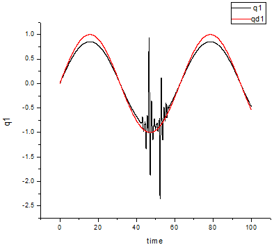
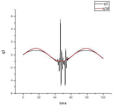
where, (i) represents the link. In this case we are considering tripe link i.e, maximum i=3. The trajectory tracking performance of the proposed control law with respect to desired position angle for each link of TLP is given in Figure 4, represented as $q_{-} d(i)$ where i=1 to 3.
The CTC technique is also implemented on the TLP in order to compare results of proposed controller technique. The trajectory tracking performance of each link of TLP with respect to desired trajectory of TLP on applying CTC controller is represented in Figure 5.
(a) Tracking performance for first link
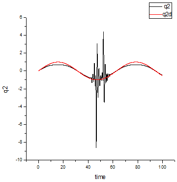
(b) Tracking performance for second link
(c) Tracking performance for third link
Figure 4. Trajectory Tracking Performance for Triple Link Pendulum (a) First Link, (b) Second link, (c) Third Link on applying proposed robust control law with respect to desired each link trajectory
(a) Tracking Performance for first link
(b) Tracking Performance for Second Link
(c) Tracking Performance for Third Link
Figure 5. Trajectory Tracking Performance for Triple Link Pendulum (a) First Link, (b) Second link, (c) Third Link on applying computed torque control (CTC) technique with respect to desired each link trajectory
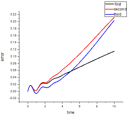
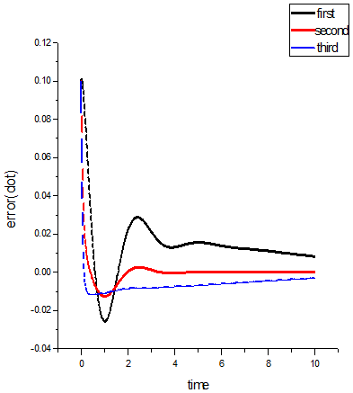
(a) Position error for first link
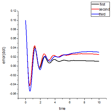
(b) Velocity error for Second Link
Figure 6. Trajectory Tracking Error Performance for Triple Link Pendulum (a) Position error performance of Triple Link Pendulum (b) Velocity error performance of Triple Link Pendulum on applying computed torque control (CTC) technique
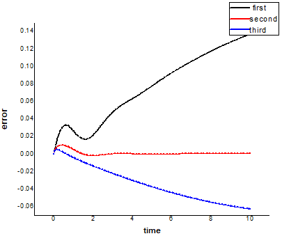
It is clear that in case of robust controller disturbance are much higher CTC controller. The performance estimation of both the controllers (CTC and Proposed Robust Control technique) can be estimated with respect to their tracking error. The position tracking error and velocity tracking error for CTC Technique can be seen in Figure 6 whereas for proposed Robust Control Technique can be seen in Figure 7.
From Figure 6 and 7 it is clear that error in case of CTC is much more than Robust based Control technique for each link. This validates the effectiveness of the proposed controller.
(a) Position error for first link
(b) Velocity error for Second link
Figure 7. Trajectory Tracking Error Performance for Triple Link Pendulum (a) Position error performance of Triple Link Pendulum (b) Velocity error performance of Triple Link Pendulum on applying proposed robust control
A novel UUB was proposed for tracking control of robot manipulator. It can be concluded that the proposed robust control law improved the tracking error and stability of the system. In order to test the trajectory tracking of triple link pendulum CTC and Proposed Robust control technique was implemented in triple link distributed pendulum system. This research proves that proposed robust control provides better trajectory tracking result with comparison to standard CTC. In future one can apply this technique to more degree of freedom manipulator.
Author thanks to Dr. Teng-Hu Cheng Assistant Professor at Dept. of Mechanical Engineering, NCTU, Hsinchu, Taiwan for providing conceptual information on nonlinear control.
The Lagrangian of TLDP is given as follows:
$\begin{align} & \\ & L=\frac{{{I}_{c1}}\dot{\theta }_{1}^{2}}{2}+\frac{{{m}_{1}}l_{1}^{2}\dot{\theta }_{1}^{2}}{8}+\frac{{{I}_{c2}}\dot{\theta }_{2}^{2}}{2}+\frac{{{m}_{2}}}{2}[l_{1}^{2}\dot{\theta }_{1}^{2}+\frac{l_{2}^{2}\dot{\theta }_{2}^{2}}{4}+ \\ & {{l}_{1}}{{l}_{2}}{{{\dot{\theta }}}_{1}}{{{\dot{\theta }}}_{2}}\cos ({{\theta }_{1}}-{{\theta }_{2}})]+\frac{{{I}_{c3}}\dot{\theta }_{3}^{2}}{2}+\frac{{{m}_{3}}}{2}[l_{1}^{2}\dot{\theta }_{1}^{2}+l_{2}^{2}\dot{\theta }_{2}^{2}+\frac{l_{3}^{2}\dot{\theta }_{3}^{2}}{4} \\ & +2{{l}_{1}}{{l}_{2}}\cos ({{\theta }_{1}}-{{\theta }_{2}}){{{\dot{\theta }}}_{1}}{{{\dot{\theta }}}_{2}}+{{l}_{1}}{{l}_{3}}{{{\dot{\theta }}}_{1}}{{{\dot{\theta }}}_{3}}\cos ({{\theta }_{1}}-{{\theta }_{3}}) \\ & +{{l}_{2}}{{l}_{3}}{{{\dot{\theta }}}_{2}}{{{\dot{\theta }}}_{3}}\cos ({{\theta }_{2}}-{{\theta }_{3}})]+\frac{{{m}_{1}}g{{l}_{1}}\cos {{\theta }_{1}}}{2}+ \\ & {{m}_{2}}g({{l}_{1}}\cos {{\theta }_{1}}+\frac{{{l}_{2}}}{2}\cos {{\theta }_{2}}) \\ & +{{m}_{3}}g({{l}_{1}}\cos {{\theta }_{1}}+{{l}_{2}}\cos {{\theta }_{2}}+\frac{{{l}_{3}}}{2}\cos {{\theta }_{3}})- \\ & \frac{{{m}_{1}}g{{l}_{1}}}{2}-{{m}_{2}}g({{l}_{1}}+\frac{{{l}_{2}}}{2})-{{m}_{3}}g({{l}_{1}}+{{l}_{2}}+\frac{{{l}_{3}}}{2}) \\ \end{align}$
[1] Abooee, A., Sedghi, F., Dosthosseini, R. (2018). Design of adaptive-robust finite-time nonlinear control inputs for uncertain robot manipulators. In 2018 6th RSI International Conference on Robotics and Mechatronics (IcRoM), pp. 375-381. https://doi.org/10.1109/ICRoM.2018.8657600
[2] Adhikary, N., Mahanta, C. (2018). Sliding mode control of position commanded robot manipulators. Control Engineering Practice, 81: 183-198. https://doi.org/10.1016/j.conengprac.2018.09.011
[3] Ahanda, J.J.B.M., Mbede, J.B., Melingui, A., Essimbi, B. (2018). Robust adaptive control for robot manipulators: Support vector regression-based command filtered adaptive backstepping approach. Robotica, 36(4): 516-534. https://doi.org/10.1017/S0263574717000534
[4] Ahangarian Abhari, S., Hashemzadeh, F., Baradarannia, M., Kharrati, H. (2019). An adaptive robust control scheme for robot manipulators with unknown backlash nonlinearity in gears. Transactions of the Institute of Measurement and Control, 41(10): 2789-2802. https://doi.org/10.1177/0142331218810773
[5] Laxmidhar, B., Indrani, K. (2009). Intelligent Systems and Control Principals and Applications. Oxford University Press, Inc.198 Madison Ave. New York, NYUnited States.
[6] Fateh, M.M. (2010). Proper uncertainty bound parameter to robust control of electrical manipulators using nominal model. Nonlinear Dynamics, 61(4): 655-666. https://doi.org/10.1007/s11071-010-9677-7
[7] Fu, L.C. (1992). Robust adaptive decentralized control of robot manipulators. IEEE Transactions on Automatic Control, 37(1): 106-110. https://doi.org/10.1109/9.109643
[8] Galicki, M. (2016). Finite-time trajectory tracking control in a task space of robotic manipulators. Automatica, 67: 165-170. https://doi.org/10.1016/j.automatica.2016.01.025
[9] Gupta, M.K., Bansal, K., Singh, A.K. (2014). Stabilization of triple link inverted pendulum system based on LQR control technique. In International Conference on Recent Advances and Innovations in Engineering (ICRAIE-2014), pp. 1-5. https://doi.org/10.1109/ICRAIE.2014.6909204
[10] Gupta, M.K., Sinha, N., Bansal, K., Singh, A.K. (2016). Natural frequencies of multiple pendulum systems under free condition. Archive of Applied Mechanics, 86(6): 1049-1061. https://doi.org/10.1007%2Fs00419-015-1078-4
[11] Ham, C., Qu, Z., Johnson, R. (2000). Robust fuzzy control for robot manipulators. IEE Proceedings-Control Theory and Applications, 147(2): 212-216. https://doi.org/10.1049/ip-cta:20000152
[12] Islam, S., Liu, X.P. (2010). Robust sliding mode control for robot manipulators. IEEE Transactions on Industrial Electronics, 58(6): 2444-2453. https://doi.org/10.1109/TIE.2010.2062472
[13] Kolhe, J.P., Shaheed, M., Chandar, T.S., Talole, S.E. (2013). Robust control of robot manipulators based on uncertainty and disturbance estimation. International Journal of Robust and Nonlinear Control, 23(1): 104-122. https://doi.org/10.1002/rnc.1823
[14] Lin, F., Brandt, R.D. (1998). An optimal control approach to robust control of robot manipulators. IEEE Transactions on Robotics and Automation, 14(1): 69-77. https://doi.org/10.1109/70.660845
[15] Liu, G.J., Goldenberg, A.A. (1996). Asymptotically stable robust control of robot manipulators. Mechanism and Machine Theory, 31(5): 607-618. https://doi.org/10.1016/0094-114X(95)00098-J
[16] Liu, G., Goldenberg, A.A. (1996). Uncertainty decomposition-based robust control of robot manipulators. IEEE Transactions on Control Systems Technology, 4(4): 384-393. https://doi.org/10.1109/87.508886
[17] Nakamura, Y., Hanafusa, H. (1987). Optimal redundancy control of robot manipulators. The International Journal of Robotics Research, 6(1): 32-42. https://doi.org/10.1177/027836498700600103
[18] Pan, H., Xin, M. (2014). Nonlinear robust and optimal control of robot manipulators. Nonlinear Dynamics, 76(1): 237-254. https://doi.org/10.1007/s11071-013-1123-1
[19] Slotine, J.J.E. (1985). The robust control of robot manipulators. The International Journal of Robotics Research, 4(2): 49-64. https://doi.org/10.1177/027836498500400205
[20] Spong, M.W. (1992). On the robust control of robot manipulators. IEEE Transactions on Automatic Control, 37(11): 1782-1786. https://doi.org/10.1109/9.173151
[21] Swarup, A., Gopal, M. (1989). Control strategies for robot manipulators—a review. IETE Journal of Research, 35(4): 198-207. https://doi.org/10.1080/03772063.1989.11436815
[22] Tao, G. (1992). On robust adaptive control of robot manipulators. Automatica, 28(4): 803-807. https://doi.org/10.1016/0005-1098(92)90040-M
[23] Wen, J.T., Murphy, S.H. (1990). PID control for robot manipulators. Rensselaer Polytechnic Institute, CIRSSE Document, 54: 1-17.
[24] Xu, J., Qiao, L. (2013). Robust adaptive PID control of robot manipulator with bounded disturbances. Mathematical Problems in Engineering, 2013: 535437. https://doi.org/10.1155/2013/535437