Lamyae Fahmani* | Siham Benhadou | Hicham Medromi
© 2021 IIETA. This article is published by IIETA and is licensed under the CC BY 4.0 license (http://creativecommons.org/licenses/by/4.0/).
OPEN ACCESS
The Unmanned Aerial Vehicle (UAV) has justified its effectiveness in electric transmission lines inspection by their great ability to perform precise, fast, and easy missions’ inspection. Due to the specification of our mission, which is the presence of electromagnetic interference in the vicinity of the transmission lines, and to avoid any deviation, crushing, or damage, it is necessary to study the safety of the UAV system and its attitude estimation. So, this paper presents a proposed basis for the implementation of UAV in the electric transmission lines inspection to use it for its attitude study problems near transmission lines. It is necessary to begin our study with the mathematical modeling, to study the physical efforts, the affecting parameters, and the behavior of the system, therefore, the mathematical model of a multirotor UAV is presented, which is the adequate UAV type that was chosen in our previous work, by justifying the choice of the quaternions mathematical approach and its simulation using the PID controller. We calculate the magnetic field near electric transmission lines using the image theorem and to ensure stable, reliable, and safe flight under electromagnetic interferences, we use the Extended Kalman Filter (EKF) by incorporating the magnetic equations in the form of colored noise. So, this proposed basis can be used to study the attitude problems of electric transmission lines inspection’s UAV.
electromagnetic interferences, extended Kalman filter, quaternions, transmission lines inspection, unmanned aerial vehicle
This paper is an extension of work originally presented in the 1st International Conference on Innovative Research in Applied Science, Engineering and Technology [1], where more results have been added, justified the choices, and expanded discussions.
The development of Unmanned Aerial Vehicles (UAVs) technologies let their use in different fields increases, they became the first choice for several applications, like remote sensing [2], agriculture [3], monitoring air pollution [4], 3D mapping [5], fire detection [6], thanks to their different advantages and capabilities [7]. This is the case for the electric transmission lines inspection, the use of UAVs was adopted by different operators as they have demonstrated their great ability to perform precise, fast, and easy inspections of power lines by comparing with the different inspection methods [6, 8], such as: Patrols, Manned Aerial Vehicle [9-11], and Rolling on Wire Robots [12, 13].
The use of UAVs makes possible to detect and locate the various defects in transmission lines by processing aerial images and videos and to have a real-time reading of the captured data. They reduce cost, time, manpower, and logistical means and they improve the reliability and quality of the operation, and above all, they secure the linemen as they will not need to approach to the lines [8].
The electric transmission lines inspection is a specific mission given its requirements and characteristics. This is why it is necessary to make a good study to choose the most suitable type of UAV and to establish a solid mathematical model in order to ensure the good progress of the mission while achieving the expected objectives.
By a comparative study of the different types of existing UAVs: the fixed wings UAV, the vertical take-off and landing, and the convertible UAV, and from a practical study of UAVs that was used or tested in electric transmission lines, that have been already presented by Fahmani et al. [1], the adequate choice of UAV’s type have been justified. A multirotor with at least four rotors was considered to be a good solution for establishing vertical and horizontal inspections with great maneuverability.
The presence in the vicinity of the electric transmission lines puts the UAV under several risks. In addition to the possibility of getting stuck or crashing with any line’s component, electromagnetic interferences caused by the lines can interfere with UAV’s radio signals, causing it to deviate from its path or crash. This can endanger anyone below or damage the UAV or the power lines [14]. And, when the UAV flying close to the electric transmission lines, there are risks of flashover through the UAV or corona discharge on the UAV because of the electric field disturbance caused by the UAV [15]. Hence the obligation to leave a safe distance between the UAV and electric lines.
There are many research studies that have addressed this interference problem to ensure the safety and smooth running of inspection missions. Some work has simply considered a safe distance, and there are others that have focused on electromagnetic simulations or laboratory tests to analyze the resistance to electromagnetic interference of its electronic circuits and communication signals [16].
Several works implement the EKF to UAVs to study their attitude estimation to have more stability and security during the flight [17-21], and given our mission type’s risks, the warranty of having a stable, reliable, and secure flight will be vital. So, this paper is interested by the study of the attitude estimation of the electric transmission lines inspection’s UAV using the EKF by incorporating the magnetic equations in the form of colored noise [22].
So, firstly, the mathematical model of a multirotor UAV will be presented by justifying the choice of the mathematical approach of quaternions, with a simulation under Matlab/Simulink with a PID controller. After that, the calculation of magnetic field will be elaborated in the vicinity of electric transmission lines using the image theorem. Finally, the Extended Kalman Filter will be presented to guarantee a stable, reliable and secure flight, by the incorporating of the magnetic equations as colored noise to have a proposed mathematical basis of the mathematical model and the Extended Colored Kalman Filter (ECKF) model of a multirotor UAV of electric transmission lines inspections.
To develop the multirotor mathematical model, it is necessary to define first of all: the hypotheses to be considered, frames, forces, torques, which is already done by Fahmani et al. [1], and the mathematical approach to be used.
So, below the different mathematical approach existed will be presented to choose the most suitable.
2.1 Mathematical approaches
Generally, there are two methods for determining the multirotors UAV’s motion equations:
2.1.1 Newton-Euler model
Newton-Euler dynamic equations are based on forces and moments, whose equations, Newton and Euler’s dynamic equations, are evaluated numerically and recursively [23]. It states that the sum of forces and torques acting on each link cause the variations in linear and angular momentums [24].
It is a fast model in calculation and control and it is better for the implementation of control schemes.
Newton’s Dynamic Equation:
$\sum F_{i}=\frac{d(m V)}{d t}$ (1)
In the inertial frame:
$m \ddot{\xi}=\sum F_{i}$ (2)
$\sum F_{\text {mobile }}=T^{T} Weight + Forces $ (3)
$\sum F_{\text {Earthly }}= Weight + T.Forces $ (4)
Euler’s Dynamic Equation:
$\sum M_{i}=\frac{d(I \omega)}{d t}$ (5)
In the body frame:
$\sum \overrightarrow{M_{O}}=\frac{d(I \vec{\omega})}{d t}=\frac{d\left(\overrightarrow{L_{O}}\right)}{d t}$ (6)
With $\overrightarrow{L_{o}}$ is the kinetic moment.
$\overrightarrow{L_{O}}=\overrightarrow{O M} \wedge m \vec{V}=\mid \vec{\omega}$ (7)
If the frame is not Galilean:
$\frac{d\left(\overrightarrow{L_{o}}\right)}{d t}=\sum \overrightarrow{M_{0}}+$$\overrightarrow{M_{O}}$$\overrightarrow{\left(f_{\text {inertia }}\right)}$ (8)
So, from the Newton and Euler’s dynamic equations the equations systems can be deduced.
2.1.2 Euler-Lagrange model
This model allows the system analyze, as a whole, based on its kinetic and potential energy. It is based on the relation between the Lagrangian and the generalized external forces that is presented in the Eq. (15). It is better adopted in the study of dynamic properties and in the analysis of control schemes. The Lagrange equations stay invariant related to all the generalized coordinates used [23].
By the Lagrangian L, motion equations can be determined in a systematic way and independently of the frame that we have chosen. It is an explicit function of the generalized coordinates $q_{i}$, generalized velocities $\dot{q}_{l}$, and time t:
$L=L\left(q_{i}, \dot{q}_{l}, t\right)$ (9)
where: $q=(\xi, \eta)^{T}$ and
$L=E_{\text {trans }}+E_{\text {rot }}-E_{P}$ (10)
with:
$E_{\text {trans }}=\frac{1}{2} m \dot{\xi}^{T} \dot{\xi}$ (11)
$E_{\text {rot }}=\frac{1}{2} \dot{\eta}^{T} J \dot{\eta}$ (12)
$E_{p}=m G z$ (13)
so:
$L\left(q_{i}, \dot{q}_{l}\right)=\frac{1}{2} m \dot{\xi}^{T} \dot{\xi}+\frac{1}{2} \dot{\eta}^{T} J \dot{\eta}-m G z$ (14)
also:
$F^{\prime}=\frac{d}{d t} \frac{\delta L}{\delta \dot{q}}-\frac{d L}{d q}$ (15)
As the Lagrangian does not contain any crossed terms in the kinetic energy combination, the Euler-Lagrange equation can be divided on two equations:
$m \ddot{\xi}+\left(\begin{array}{c}0 \\ 0 \\ m g\end{array}\right)=F_{\xi}$ (16)
$J \ddot{\eta}+\dot{J} \dot{\eta}-\frac{1}{2} \frac{\delta}{\delta \eta}\left(\dot{\eta}^{T} J \dot{\eta}\right)=\tau$ (17)
So, from the two equations above the equations systems can be deduced.
Returning to transformation matrices if we calculate the inverse of the matrix W, we find that it is written as follows:
$W^{-1}=\left(\begin{array}{ccc}1 & 0 & 0 \\ t_{\theta} s_{\phi} & c_{\phi} & s c_{\theta} s_{\phi} \\ t_{\theta} c_{\phi} & -s_{\phi} & s c_{\theta} c_{\phi}\end{array}\right)$ (18)
where, $t_{\theta}=\tan \theta$ and $s c_{\theta}=\sec \theta=\frac{1}{\cos \theta}$.
It is defined if and only if: $\theta \neq \frac{\pi}{2}+k \pi,(k \in \mathbb{Z})$, because of the term $\theta$. Hence the generation of a singular point (Gimbal Lock) this means the loss of a freedom degree.
2.1.3 Quaternions
So, to overcome the problem of a singular point, different presentations can be considred such as the Quaternions where the rotation in one frame regarding another frame will be presented by 4 parameters ($\mathrm{q}_{0}, \mathrm{q}_{1}, \mathrm{q}_{2}, \mathrm{q}_{3}$), and the advantages of using an approach based on it consist not only in the absence of singularities but also in the simplicity of computation.
The transformation matrix $T_{Q}$ from the initial frame $\left(X_{B}, Y_{B}, Z_{B}\right)$ to the relative frame $\left(x_{R}, y_{R}, z_{R}\right)$ of coordinates is presented below [1]:
$T_{Q}=\left(\begin{array}{ccc}q_{0}^{2}+q_{1}^{2}-q_{2}^{2}-q_{3}^{2} & 2\left(q_{0} q_{3}+q_{1} q_{2}\right) & 2\left(q_{1} q_{3}-q_{0} q_{2}\right) \\ 2\left(q_{1} q_{2}-q_{0} q_{3}\right) & q_{0}^{2}+q_{2}^{2}-q_{1}^{2}-q_{3}^{2} & 2\left(q_{0} q_{1}+q_{2} q_{3}\right) \\ 2\left(q_{0} q_{2}+q_{1} q_{3}\right) & 2\left(q_{2} q_{3}-q_{0} q_{1}\right) & q_{0}^{2}+q_{3}^{2}-q_{1}^{2}-q_{2}^{2}\end{array}\right)$ (19)
2.2 Multirotors dynamic model
It is already presented in detail in [16] the different expressions of forces and moments undergone by a multirotor UAV of the quadcopter type and formulations which are used to deduce the equations systems below of the adopted quadcopter:
$\left\{\begin{array}{c}\ddot{x}=-\frac{K_{f t x}}{m} \dot{x}+\frac{2}{m}\left(q_{1} q_{3}-q_{0} q_{2}\right) \sum_{i=1}^{n} b \omega_{i}^{2} \\ \ddot{y}=-\frac{K_{f t y}}{m} \dot{y}+\frac{2}{m}\left(q_{0} q_{1}-q_{2} q_{3}\right) \sum_{i=1}^{n} b \omega_{i}^{2} \\ \ddot{z}=-G-\frac{K_{f t z}}{m} \dot{z}+\frac{1}{m}\left(q_{0}^{2}+q_{3}^{2}-q_{1}^{2}-q_{2}^{2}\right) \sum_{i=1}^{n} b \omega_{i}^{2} \\ \ddot{\phi}=\frac{M_{x}}{I_{x}}-\frac{K_{f a x}}{I_{x}} \dot{\phi}^{2}-\frac{\Omega_{r} J_{r}}{I_{x}} \dot{\theta}-\dot{\theta} \dot{\psi}\left(\frac{I_{z}-I_{y}}{I_{x}}\right) \\ \ddot{\theta}=\frac{M_{y}}{I_{y}}-\frac{K_{f a y}}{I_{y}} \dot{\theta}^{2}+\frac{\Omega_{r} J_{r}}{I_{y}} \dot{\phi}-\dot{\psi} \dot{\phi}\left(\frac{I_{x}-I_{z}}{I_{y}}\right) \\ \ddot{\psi}=\frac{M_{z}}{I_{z}}-\frac{K_{f a z}}{I_{z}} \dot{\psi}^{2}-\dot{\phi} \dot{\theta}\left(\frac{I_{y}-I_{x}}{I_{z}}\right)\end{array}\right.$ (20)
With:
$\Omega_{r}=\sum_{i=1}^{n}(-1)^{i+1} \omega_{i}$ (21)
$\left(\begin{array}{lll}M_{x} & M_{y} & M_{z}\end{array}\right)^{T}$ is the drag moment where:
$M_{Z}=d \Omega_{r}$ (22)
And, for $M_{x}$ and $M_{y}$, we will present below their expressions according to three different configurations of multirotor:
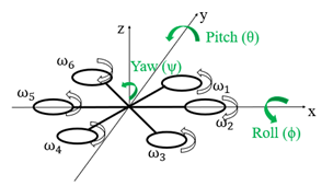
2.2.1 Quadcopter
The Figure 1 presents the adopted quadcopter’s diagram, from which we can deduce the following equations:
$M_{x}=b l\left(\omega_{1}^{2}-\omega_{3}^{2}\right)$ (23)
$M_{y}=b l\left(\omega_{4}^{2}-\omega_{2}^{2}\right)$ (24)
2.2.2 Hexacopter
The Figure 2 presents the adopted hexacopter’s diagram, from which we can deduce the following equations:
$M_{x}=b l\left(\omega_{5}^{2}-\omega_{2}^{2}+\frac{1}{2}\left(\omega_{1}^{2}+\omega_{3}^{2}-\omega_{4}^{2}-\omega_{6}^{2}\right)\right)$ (25)
$M_{y}=\frac{\sqrt{3}}{2} b l\left(\omega_{1}^{2}+\omega_{3}^{2}-\omega_{4}^{2}-\omega_{6}^{2}\right)$ (26)
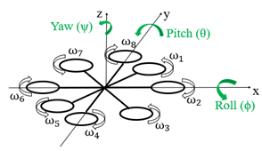
2.2.3 Octocopter
The Figure 3 presents the adopted octocopter’s diagram, from which we can deduce the following equations:
$M_{x}=b l\left(\omega_{6}^{2}-\omega_{2}^{2}+\frac{\sqrt{2}}{2}\left(\omega_{1}^{2}+\omega_{3}^{2}-\omega_{5}^{2}-\omega_{7}^{2}\right)\right)$ (27)
$M_{y}=b l\left(\omega_{4}^{2}-\omega_{8}^{2}+\frac{\sqrt{2}}{2}\left(\omega_{1}^{2}+\omega_{7}^{2}-\omega_{3}^{2}-\omega_{5}^{2}\right)\right)$ (28)
For our simulation, we chose the quadcopter presented in Figure 1, with the system’s parameter values those presented by Khebbache [25], based on M. Abdel-Razzak model [26] which is a Simulink model of a quadcopter with a PD controller.
To represent our system, it was adapted with the quaternion approach by adding the aerodynamic effects and an integral regulator to improve the steady-state.
Figure 1. The quadcopter’s diagram adopted
Figure 2. The hexacopter’s diagram adopted
Figure 3. The octocopter’s diagram adopted
So, in Figures below 4-11, the results of the first simulation are presented, where we fixed the desired values of the system’s variables, and using a random values of the PID regulator.
Figure 4. The first simulation result of the quaternion coordinate $q_{0}$
Figure 5. The first simulation result of the quaternion coordinate $q_{1}$
Figure 6. The first simulation result of the quaternion coordinate $q_{2}$
Figure 7. The first simulation result of the quaternion coordinate $q_{3}$
Figure 8. The first simulation result of $\varphi(r a d)$
Figure 9. The first simulation result of $\theta(\mathrm{rad})$
Figure 10. The first simulation result of $\Psi(\mathrm{rad})$
Figure 11. The first simulation result of the altitude z(m)
The values of the PID regulator influence the stabilization of the system, therefore since the output values do not follow the desired values therefore the values of the regulator are incorrect. So, you have to vary these values until we have the correct values, that will give us a stable, accurate and fast system.
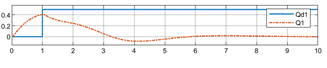
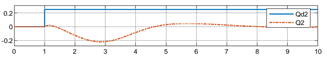
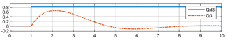
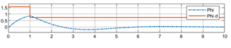
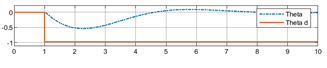
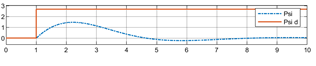
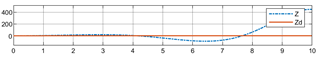
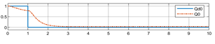
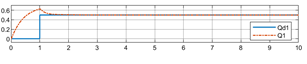
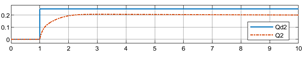
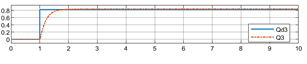
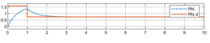
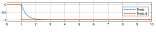
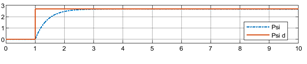
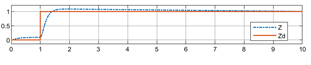
In Figures 12-19, the final simulation of the system parameters is presented with the accurate values of the parameters P, I and D, where we have a good tracking of the desired values with small transient deviations.
Figure 12. The final simulation result of the quaternion coordinate $q_{0}$
Figure 13. The final simulation result of the quaternion coordinate $q_{1}$
Figure 14. The final simulation result of the quaternion coordinate $q_{2}$
Figure 15. The final simulation result of the quaternion coordinate $q_{3}$
Figure 16. The final simulation result of $\varphi(r a d)$
Figure 17. The final simulation result of $\theta(\mathrm{rad})$
Figure 18. The final simulation result of $\Psi(\mathrm{rad})$
Figure 19. The final simulation result of the altitude z(m)
The presence of the UAV near high-voltage electric transmission lines will cause it to be subjected to the propagation of electromagnetic waves, which has many effects on materials and communication signals. That is why the calculation of the magnetic field in the vicinity of the transmission lines is necessary.
There are several methods adopted to calculate the magnetic field in the vicinity of transmission lines, such as the Biot-Savart laws [22, 27], the finite element method [28], and the image theorem that has been well detailed in Fahmani et al. [16].
So, from Fahmani et al. [16], we took the expression for the magnetic field using the image theorem for the case of a 400 kV double-circuit overhead power line supported by an S-pylon, which is the extreme case of the Moroccan electrical transmission network.
$\overrightarrow{B_{M}}(x, y)=\sum_{i=1}^{N} \frac{\mu_{0} I_{i}}{2 \pi}\left(\frac{\overrightarrow{l_{l}} \wedge \overrightarrow{R_{l}}}{R_{i}^{2}}-\frac{\overrightarrow{l_{l}^{\prime}} \wedge \overrightarrow{R_{l}^{\prime}}}{R_{i}^{\prime} 2}\right)$ (29)
$\overrightarrow{B_{M}}(x, y)$$=\left\{\begin{array}{c}B_{M_{x}}(x, y)=\sum_{i=1}^{N} \frac{\mu_{0} I_{i}}{2 \pi}\left(\begin{array}{c}\frac{y-y_{i}}{R_{i}^{2}} \\ -\frac{y+y_{i}+\delta(1-j)}{R^{\prime}{ }_{i}^{2}}\end{array}\right) \\ B_{M_{y}}(x, y)=\sum_{i=1}^{N} \frac{\mu_{0} I_{i}\left(x-x_{i}\right)}{2 \pi}\left(\frac{1}{R_{i}{ }^{2}}-\frac{1}{{R^{\prime}}_{i}^{2}}\right)\end{array}\right.$ (30)
So,
$\left|B_{M x}(x, y)\right|=$$=\sqrt{\left|\sum_{i=1}^{N} \frac{\mu_{0} I_{i}}{2 \pi}\left(\frac{y-y_{i}}{R_{i}^{2}}-\frac{y+y_{i}+\delta}{R_{i}^{\prime}{ }^{2}}\right)\right|^{2}+\left|\sum_{i=1}^{N} \frac{\mu_{0} I_{i}}{2 \pi} \frac{\delta}{R^{\prime}{ }_{i}^{2}}\right|^{2}}$ (31)
$\left|B_{M y}(x, y)\right|=\left|\sum_{i=1}^{N} \frac{\mu_{0} I_{i}\left(x-x_{i}\right)}{2 \pi}\left(\frac{1}{R_{i}^{2}}-\frac{1}{R^{\prime}{ }^{2}}\right)\right|$ (32)
$\left|B_{M}(x, y)\right|=\left|\overrightarrow{B_{M}}(x, y)\right|=\sqrt{\frac{\left|B_{M x}(x, y)\right|^{2}}{\prod}}+\left|B_{M y}(x, y)\right|^{2}$ (33)
And to express it in the body frame we must just multiply it by the transformation matrix T:
$B_{M_{B}}=T B_{M}$ (34)
Therefore, it can be represented by a function which depends on the position and the quaternions coordinates as indicated in the following equation:
$B_{M_{B}}=h\left(x, y, z, q_{0}, q_{1}, q_{2}, q_{3}\right)$ (35)
5.1 The extended Kalman filter’s introduction
Kalman Filter (KF) is an optimal estimation algorithm that predicts a parameter of interests such as location, speed, and direction in the presence of noise and measurements. It is used when the variables of interest can only be measured indirectly, and when the measurements are available from various sensors but might be subject to noise [29]. The KF is defined only for linear systems. So, for non-linear systems its non-linear version, that is called the Extended Kalman Filter (EKF), can be used.
To guarantee a stable, reliable and secure flight, the EKF was used in several works to UAVs. And among so many nonlinear filters, EKF is the most widely used and the simplest filter [18]. But, to apply it to our case, we must take into consideration our specific conditions due to the permanent presence near electric transmission lines. This electromagnetic interference at the vicinity of transmission lines is presented [22] like a non-Gaussian time-variant noise with nonzero mean value and they studied this type of noise by the approach of colored noise.
So, in the following, the presentation of the necessary adaptations and the final mathematical formulation applied to Extended Colored Kalman Filter (ECKF) by the incorporating of the magnetic equations as colored noise in a traditional EKF along with the flight dynamics of the vehicle based on the quaternions.
The principle of Kalman Filter is to find the probability of the hypothesis of predicted state is given by hypothesis of prior state and then using the data from measurement sensor to correct the hypothesis to get the best estimation for each time [30]. So, it combines the measurement and the prediction to find the optimal estimation in the presence of process and measurement noise.
The most important part of applying EKF is the model and there are two models for EKF for the case of a nonlinear discrete time system with linear measurement [22, 31]:
State Model:
$x_{k}=f\left(x_{k-1}, u_{k}\right)+\varepsilon_{k}$ (36)
Measurement Model:
$y_{k}=H_{k} x_{k}+v_{k}$ (37)
$v_{k}$ is a nonzero mean with a nonlinear variation, is the colored noise:
$v_{k}=g\left(v_{k-1}\right)+\xi_{k}$ (38)
5.2 The extended Kalman filter’s algorithm
EKF is a recursive algorithm used for estimating a dynamic system which lacks data. It uses prior knowledge to predict the past, present, as well as future state of the system [30]. Notice that to estimate the current state, the algorithm doesn’t need all the past information. It only needs the estimated state and error covariance matrix from the previous time step and the current measurement ($\hat{x}_{k-1}, P_{k-1}, y_{k}$) [31-33].
Prediction Phase:
The a priori state estimate:
$\hat{x}_{k}^{-}=f\left(\hat{x}_{k-1}^{+}, u_{k}\right)$ (39)
The a priori error covariance matrix:
$P_{k}^{-}=F_{k} P_{k-1}{ }^{+} F_{k}^{T}+Q_{\varepsilon_{x}}$ (40)
Update Phase:
$Z_{k}=y_{k}-H_{k} \hat{x}_{k}^{-}-g\left(\hat{x}_{k}^{-}, v_{k-1}\right)-\xi_{k}$ (41)
$S_{k}=\Omega_{k} P_{k}^{-} \Omega_{k}^{T}+Q_{\xi_{k}}$ (42)
$\Omega_{k}=H_{k}+\left.\frac{\partial g}{\partial x}\right|_{\hat{x}_{k}}-$ (43)
The Kalman gain:
$K_{k}=P_{k}^{-} \Omega_{k}^{T} S_{k}^{-1}$ (44)
The a posteriori state estimate:
$\hat{x}_{k}^{+}=\hat{x}_{k}^{-}+K_{k} Z_{k}$ (45)
The a posteriori error covariance matrix:
$P_{k}^{+}=\left(I-K_{k} \Omega_{k}\right) P_{k}^{-}$ (46)
$F_{k}$ is the Jacobian of $f$:
$F_{k}=\left.\frac{\partial f}{\partial x}\right|_{\hat{x}_{k-1}}$ (47)
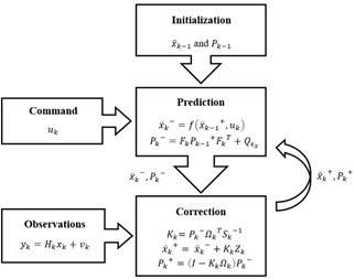
So, the EKF is a recursive algorithm, as it is presented in the Figure 20 below, that breaks down into three main steps: Initialization, Prediction, and Correction, and that has two inputs: Command and Observations [34].
Figure 20. The EKF’s algorithm
To determine the state vector $x_{k}$ and $y_{k}$ it is necessary to be interested in having a simple model and more intuitive measurements. So, for our case, the chosen state vector below presents the quaternion coordinates and the three gyroscope biases (the gyroscope is a magnetic, angular rate, and gravity sensor, and it can be used to measure the angular rate of the vehicle, and the time integration of angular rate derives the rotated angle, but the accumulation error would gradually increase as integral time increase [18]):
$x_{k}=\left(q_{0_{k}}, q_{1_{k}}, q_{2_{k}}, q_{3_{k}}, b_{x_{k}}, b_{y_{k}}, b_{z_{k}}\right)$ (48)
And:
$y_{k}=\left(q_{0_{k}}, q_{1_{k}}, q_{2_{k}}, q_{3_{k}}\right)$ (49)
By noting that the outputs data of the magnetometer and accelerometer’s UAV can give us the values of the quaternions using several methods detailed in Jing et al. [18].
In our previous work, the adequate type of UAV for transmission lines inspection have been chosen, which was the multirotor UAV with at least four rotors, by the two comparative and practical studies of the different UAV’s existing types. And, in this paper, a solid basis for the implementation of UAVs in the inspection of electric transmission lines was presented to implement it, in future works, on a real system.
To develop the mathematical model, the different mathematical approaches that existed were presented and the quaternion approach choice was proved. After that we present a general mathematical model, which can be adopt for all multirotors with four or more rotors, with its simulation under Matlab/Simulink with a PID controller.
This paper used the EKF, which combines measurement and prediction to find the optimal estimate in the presence of process and measurement noise, to ensure stable, reliable and safe flight under electromagnetic interference, by incorporating the magnetic equations in the form of colored noise.
So, this paper presented a complete equation model of the mathematical model and the ECKF model of a multirotor UAV of electric transmission lines inspections. And using this base of equations, instead of physical tests, we can plan automatic missions for electric transmission lines inspection, overcome the attitude problems of UAVs under electromagnetic interferences, and have a specific UAV that will be intended primarily for electric transmission lines inspection. The results of our work will be the subject of practical tests in future work in order to test and validate this model of equations.
This work was supported by the National Centre for Scientific and Technical Research (CNRST) and Research Foundation for Development and Innovation in Science and Engineering (FRDISI) Scientific Scholarships.
|
b |
the lift coefficient, N.rad-1.s-1 |
|
d |
the drag coefficient, N.m.rad-1.s-1 |
|
$E_{\text {trans }}$ |
the translational energy, J |
|
$E_{\text {rot }}$ |
the rotational energy, J |
|
$E_{P}$ |
the potential energy, J |
|
$F$ |
the generalized external forces, N |
|
$F^{\prime}$ |
the generalized external forces that is defined by: $F^{\prime}=\left(F_{\xi}, \tau\right)$ |
|
$F_{\xi}$ |
the translational force, N |
|
$f$ |
the nonlinear function. |
|
$f^{\prime}$ |
the nonlinear function. |
|
G |
the gravitational constant, m.s-2 |
|
g |
the nonlinear function that represents the interferences with electric transmission lines |
|
$H_{k}$ |
maps the state variables to the measurements. |
|
I |
the moment of inertia of the system, kg.m2 |
|
$I_{i}$ |
the intensity of the conductor's current, A |
|
$I_{x}, I_{y}$ and $I_{z}$ |
are respectively the moments of inertia around the $x, y$ and $z$ axis, kg.m2 |
|
$J$ |
the inertia of the system, kg.m2 |
|
$J_{r}$ |
the inertia of the rotor, kg.m2 |
|
$K_{f a}$ |
the aerodynamic friction coefficients, N.rad-1.s-1 |
|
$K_{f t}$ |
the drag coefficients, N.m-1.s-1 |
|
$K_{k}$ |
the Kalman gain |
|
l |
the length of the arm between the rotor and the multirotor’s center of gravity, m |
|
m |
the system’s mass, kg |
|
N |
the number of the conductors |
|
$P_{k}$ |
the covariance of the estimation error |
|
$P_{k}^{-}$ and $P_{k}^{+}$ |
are respectively the priori and the posteriori estimation of $P_{k}$. |
|
$R_{i}$ and $R_{i}^{\prime}$ |
are respectively the distances between the point M and the conductor i and its image, m |
|
T |
the transformation matrice |
|
$u_{k}$ |
the control data |
|
V |
the system’s velovity, m.s-1 |
|
$\left(x_{i}, y_{i}\right)$ |
the coordinates of the conductor i |
|
$x_{k}$ |
the system states |
|
$\hat{x}_{k}^{-}$ and $\hat{x}_{k}^{+}$ |
are respectively the priori and the posteriori estimation of $\hat{x}_{k}$ |
|
$y_{k}$ |
the measurement vector |
|
Greek symbols |
|
|
$(\varphi, \theta, \Psi)$ |
the Euler angles |
|
$\xi$ |
$=(x, y, z)^{T}$ |
|
$\eta$ |
$=(\varphi, \theta, \Psi)^{T}$ |
|
$\omega$ |
the system’s angular speed, rad.s-1 |
|
$\omega_{i}$ |
the angular speed of the $i^{t h}$ rotor, rad.s-1 |
|
$\tau$ |
the generalized moments, N.m |
|
$\mu_{0}$ |
the magnetic permeability of the whole space, it is taken to be the free space value and it is equal to $4 \pi \cdot 10^{-7} \mathrm{H} / \mathrm{m}$ |
|
δ |
the earth skin depth and it is equal to $\sqrt{1 /\left(\mu_{0} \pi f^{\prime} \sigma\right)}$, m |
|
σ |
the conductivity of earth, S.m-1 |
|
$\xi_{k}$ |
the white noise with zero mean correlated to g |
|
$\varepsilon_{k}$ |
the zero mean process noise with covariance $Q_{\varepsilon_{k}}$ |
|
Subscripts |
|
|
$-$ and $+$ |
are respectively the priori and the posteriori estimation |
[1] Fahmani, L., Garfaf, J., Boukhdir, K., Benhadou, S., Medromi, H. (2020). Unmanned aerial vehicles inspection for overhead high voltage transmission lines. In 2020 1st International Conference on Innovative Research in Applied Science, Engineering and Technology (IRASET), pp. 1-7. https//doi.org/10.1109/IRASET48871.2020.9092141
[2] Lucieer, A., Turner, D., King, D.H., Robinson, S.A. (2014). Using an Unmanned Aerial Vehicle (UAV) to capture micro-topography of Antarctic moss beds. International Journal of Applied Earth Observation and Geoinformation, 27: 53-62. https//doi.org/10.1016/j.jag.2013.05.011
[3] Pittu, V.R., Gorantla, S.R. (2020). Diseased area recognition and pesticide spraying in farming lands by multicopters and image processing system. J. Eur. des Syst. Autom., 53(1): 123-130. https//doi.org/10.18280/jesa.530115
[4] Alvear, O., Zema, N.R., Natalizio, E., Calafate, C.T. (2017). Using UAV-based systems to monitor air pollution in areas with poor accessibility. Journal of Advanced Transportation. https//doi.org/10.1155/2017/8204353
[5] Nex, F., Remondino, F. (2014). UAV for 3D mapping applications: a review. Applied Geomatics, 6(1): 1-15. https//doi.org/10.1007/s12518-013-0120-x
[6] Wei, Y. (2019). Design of a fire detection system based on four-rotor aircraft. Rev. d'Intelligence Artif., 33(1): 39-43. https//doi.org/10.18280/ria.330107
[7] Jordan, S., Moore, J., Hovet, S., Box, J., Perry, J., Kirsche, K., Lewis, D., Tse, Z.T.H. (2018). State-of-the-art technologies for UAV inspections. IET Radar, Sonar and Navigation, 12(2): 151-164. https//doi.org/10.1049/iet-rsn.2017.0251
[8] Li, L. (2015). The UAV intelligent inspection of transmission lines. Ameii, pp. 1542-1545. https//doi.org/10.2991/ameii-15.2015.285
[9] Ishino, R., Tsutsumi, F. (2004). Detection system of damaged cables using video obtained from an aerial inspection of transmission lines. IEEE Power Engineering Society General Meeting, 2: 1857-1862. https//doi.org/10.1109/pes.2004.1373201
[10] Luque-Vega, L.F., Castillo-Toledo, B., Loukianov, A., Gonzalez-Jimenez, L.E. (2014). Power line inspection via an unmanned aerial system based on the quadrotor helicopter. Proceedings of the Mediterranean Electrotechnical Conference - MELECON, pp. 393-397. https//doi.org/10.1109/MELCON.2014.6820566
[11] Larrauri, J.I., Sorrosal, G., Gonzalez, M. (2013). Automatic system for overhead power line inspection using an unmanned aerial vehicle - Relifo project. international Conference on Unmanned Aircraft Systems, ICUAS 2013 - Conference Proceedings, pp. 244-252. https//doi.org/10.1109/ICUAS.2013.6564696
[12] Pagnano, A., Höpf, M., Teti, R. (2013). A roadmap for automated power line inspection. maintenance and repair. Procedia CIRP, 12: 234-239. https//doi.org/10.1016/j.procir.2013.09.041
[13] Debenest, P., Guarnieri, M., Takita, K., Fukushima, E.F., Hirose, S., Tamura, K., Kimura, A., Kubokawa, H., Iwama, N., Shiga, F. (2008). Expliner - robot for inspection of transmission lines. Proceedings - IEEE International Conference on Robotics and Automation, pp. 3978-3984. https//doi.org/10.1109/ROBOT.2008.4543822
[14] Indiana Electric Cooperatives, https://www.indianaec.org/2020/05/27/drones-pose-electrical-safety-issues/#:~:text=Keep%20drones%20at%20least%20100,drone%20or%20the%20power%20lines, accessed on 6 June 2021.
[15] Liu, S., Sheng, C., Meng, F., Wang, S., Wang, R., Zhang, Y., Zhu, Y., Xu, Z., He, W. (2016). Electric field disturbance caused by an unmanned aerial vehicle flying near the HV power transmission line. IEEE International Conference on High Voltage Engineering and Application (ICHVE). https//doi.org/978-1-5090-0496-6/16/$31.00
[16] Fahmani, L., Garfaf, J., Boukhdir, K., Benhadou, S., Medromi, H. (2020). Modelling of very high voltage transmission lines inspection’s quadrotor. SN Applied Sciences, 2(8): 1-11. https//doi.org/10.1007/s42452-020-03222-y
[17] Liang, W. (2017). Attitude estimation of quadcopter through extended Kalman filter. Lehigh University, pp. 1-42.
[18] Jing, X., Cui, J., He, H., Zhang, B., Ding, D., Yang, Y. (2017). Attitude estimation for UAV using extended Kalman filter. In 2017 29th Chinese Control and Decision Conference (CCDC), pp. 3307-3312. https//doi.org/10.1109/CCDC.2017.7979077
[19] Munguía, R., Urzua, S., Grau, A. (2019). EKF-Based Parameter Identification of Multi-Rotor Unmanned Aerial Vehicles Models. Sensors (Switzerland), 19(19): pp. 1-17. https//doi.org/10.3390/s19194174
[20] Salmony, P.M. (2019). Quaternion-based extended Kalman filter for fixed-wing UAV attitude estimation. Derivation and Implementation, pp. 1-9.
[21] Wu, Y.L., Wang, T.M., Liang, J.H., Wang, C.L., Zhang, C. (2008). Attitude estimation for small helicopter using extended Kalman filter. IEEE Conference on Robotics, Automation and Mechatronics. https//doi.org/10.1109/RAMECH.2008.4690879
[22] Da Silva, M.F., Honório, L.M., Marcato, A.L.M., Vidal, V.F., Santos, M.F. (2020). Unmanned aerial vehicle for transmission line inspection using an extended Kalman filter with colored electromagnetic interference. ISA Transactions. ISA Transactions, pp. 322-333. https//doi.org/10.1016/j.isatra.2019.11.007
[23] Luukkonen, T. (2011). Modelling and control of quadcopter. Independent research project in applied mathematics, Espoo, 22.
[24] Orsag, M., Korpela, C., Oh, P. (2013). Modeling and control of MM-UAV: Mobile manipulating unmanned aerial vehicle. Journal of Intelligent & Robotic Systems, 69(1): 227-240. https//doi.org/10.1007/s10846-012-9723-4
[25] Khebbache, H. (2018). Tolérance aux défauts via la méthode backstepping des systèmes non linéaires: application système UAV de type quadrirotor (Doctoral dissertation).
[26] Math Works, https://fr.mathworks.com/matlabcentral/fileexchange/41149-pd-control-quadrotor-simulink?stid=srchtitle.
[27] Ali, Y.S.M., El-Baset, A.A., Elghaffar, A.N.A. (2016). Mathematical calculation of electromagnetic field in high voltage substations to treatment its effect on the protective EQUIPMENTS. Annals of the Faculty of Engineering Hunedoara, 14(4): 139-146.
[28] PASARE, S. (2008). Calcul du champ magnétique d'une ligne électrique aérienne à haute Tension. Annals of the University of Craiova, Electrical Engineering series, (32): 30-33.
[29] Math Works, https://fr.mathworks.com/videos/understanding-kalman-filters-part-1-why-use-kalman-filters--1485813028675.html.
[30] Keatmanee, C., Baber, J., Bakhtyar, M. (2014). Simple example of applying extended Kalman filter. 1st International Electrical Engineering Congress.
[31] Math Works, https://fr.mathworks.com/videos/understanding-kalman-filters-part-5-nonlinear-state-estimators-1495052905460.html.
[32] Math Works, https://fr.mathworks.com/videos/understanding-kalman-filters-part-4-optimal-state-estimator-algorithm--1493129749201.html.
[33] Latroch, M., Ahmed, D., Abdelhafid, O. (2019). A proposed use of kalman gains behavior of navigation measurements for the sensor fault detection in Quadcopter. Instrumentation, Mesures, Métrologies, 18(6): 567-575. https//doi.org/10.18280/i2m.180608
[34] Ndjeng Ndjeng, A. (2009). Localisation robuste multi-capteurs et multi-modèles (Doctoral dissertation, Evry-Val d'Essonne).