Hicham Zatla | Bilal Tolbi* | Fares Bouriachi
© 2021 IIETA. This article is published by IIETA and is licensed under the CC BY 4.0 license (http://creativecommons.org/licenses/by/4.0/).
OPEN ACCESS
The aim of the present research is to find an optimal reference trajectory for an underactuated manipulator of type Xn-1Rp, where X is any type of joints and R is the last rotary joint, for n≥3. It is worth noting that in the case of absence of control of fully actuated manipulator, some second-order nonholonomic constraints may appear; these are known as acceleration constraints. The second-order nonholonomic constraint is a non-integrable differential equation. For this purpose, it was decided to combine two methods. The first one provides the open-loop control of the manipulator whatever the motion time is; in practice, the motion time should be minimal under the given geometric, technological, and dynamic constraints. To address this issue, a second method, based on the offline optimization approach, was used to achieve the time-optimal motion. It was revealed that the above combination gives an optimal control trajectory for an underactuated manipulator in which a reference trajectory can be utilized.
manipulator, optimal, trajectory, nonholonomic, underactuated, planning
Over the last few years, a large number of researchers have been interested in underactuated mechanical systems that are characterized by a higher number of degrees of freedom in comparison with the number of actuators. This class of mechanical systems is naturally found, which means that the under actuation can be either intentional, i.e., for reasons of economy or weight, or unintentional in the event of failure of one or more actuators. Some examples of underactuated mechanical systems, such as the underwater vehicles, helicopters, mobiles robots, and underactuated manipulators, are worth mentioning [1].
It is worth noting that in the case of absence of control of a fully actuated manipulator, some second-order nonholonomic constraints may appear; these are known as acceleration constraints. The second-order nonholonomic constraint is a non-integrable differential equation. In this situation of constraints, it is not possible to reduce the dimension of the generalized coordinate vector [2, 3]. The control and trajectory planning for nonholonomic systems is very difficult to achieve in comparison with holonomic systems. For instance, the underactuated planar 2R manipulator with a passive last joint (no motor) is a second-order nonholonomic mechanical system.
Partial results on the control of a 2R underactuated manipulator are given in refs. [4, 5] where a motion planner was proposed for the underactuated planar 2R manipulator. It is worth reminding that De Luca and Oriolo succeeded in solving the problem of motion planning of an underactuated planar 3R manipulator based on dynamic feedback linearization [6].
The present paper aims to use the feedback linearization of a type Xn-1Rp manipulator where X is any type of active joint and R is the last rotoid passive joint [6]. It then proposes an offline optimization for the purpose of identifying the optimal time for the displacement of the manipulator from the initial configuration to the final desired configuration.
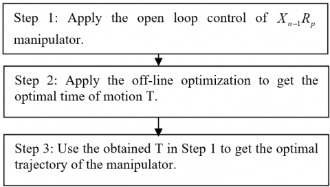
Figure 1. Diagram of the proposed method
This section presents the method applied for the purpose of obtaining the optimal control of an underactuated manipulator. In order to achieve that goal, it was first required to determine the open-loop control of the robot manipulator, then to explain the off-line optimization in order to obtain the optimal time T, Figure 1 shows the different steps of the proposed method.
2.1 Open-loop control of Xn-1Rp manipulator
The exact feedback linearization may be viewed as a suitable solution to the problem. To start, a set of linear outputs are to be defined as follows: Z=h(q), $Z \in R^{m}$.
In this case, all states and inputs can be written in term of Z and its derivatives. It then becomes possible to construct a dynamic compensator of the form:
$\dot{\zeta }=\alpha (\zeta ,q,\dot{q})+\beta (\zeta ,q,\dot{q})\nu $ (1)
$a=\gamma (\zeta ,q,\dot{q})+\delta (\zeta ,q,\dot{q})\nu$ (2)
2.1.1 Dynamic model of Xn-1Rp manipulator
where, the state $\xi \in R^{V}$ and $v \in R^{m}$ is the new input so that the closed-loop system is linear and decoupled in input-state-output. In this case, the system may be represented by m integrators between v and z. Assuming that the system has two inputs (m=2), the linearizing algorithm proceeds as follows. The two linearizing outputs z1 and z2 are differentiated repeatedly until at least an input is found in each of them. If the matrix multiplying the inputs at this differentiation level is nonsingular, then static state feedback can be used in order to linearize the input-output behavior. However, if the sum of the orders of the output derivatives is equal to the dimension of the state space, then the full state linearization is achieved [6].
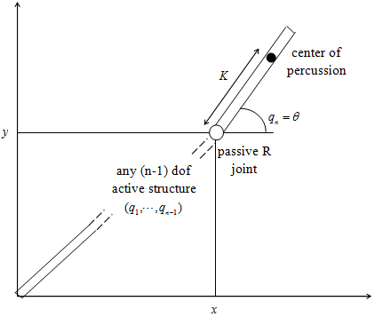
Let q=(q1, ..., qn) be any set of coordinates in a way that qn=θ is the last link orientation relative to the x axis as illustrated in Figure 2. The dynamic model can therefore be written as:
$B(q)\ddot{q}+C(q,\dot{q})+g(q)=\left[ \begin{matrix} \tau \\ 0 \\ \end{matrix} \right]$ (3)
where, the torque vector τ=(τ1, ..., τn-1) corresponds to the active links. Moreover, B(q) represents a positive symmetric inertia matrix, $C(q, \dot{q})$ is the coriolis and centrifugal force vector, and g(q) denotes all gravity terms. For the sake of simplifying the analysis of the dynamic model, the generalized coordinates used are defined by the vector: q=(q1, ..., qn-1), x, y, θ)≡(qa, θ).
Figure 2. Representation of an Xn-1Rp robot manipulator [6]
Note that x and y are the cartesian coordinates of the base of the passive axis and θ represents the orientation of that axis with respect to the x axis. The first step consisted of transforming the dynamic model into the coordinate model (x, y, θ). For this, let sθ=sinθ and cθ=cosθ; then the dynamic model Eq. (3) may be expressed in the following form:
$\left[ \begin{matrix} {{B}_{a}}({{q}_{a}}) & {} & {} & {{0}_{n-3}} \\ {} & {} & {} & -{{m}_{n}}{{d}_{n}}s\theta \\ {} & {} & {} & {{m}_{n}}{{d}_{n}}c\theta \\ 0_{n-3}^{T} & -{{m}_{n}}{{d}_{n}}s\theta & {{m}_{n}}{{d}_{n}}c\theta & {{I}_{n}}+{{m}_{n}}d_{n}^{2} \\ \end{matrix} \right]\left[ \begin{matrix} {{{\ddot{q}}}_{a}} \\ {} \\ {} \\ {\ddot{\theta }} \\ \end{matrix} \right]+ \\ \left[ \begin{matrix} {{C}_{a}}(q,\dot{q} \\ {} \\ {} \\ 0 \\ \end{matrix} \right]+\left[ \begin{matrix} {{g}_{a}}({{q}_{a}}) \\ {} \\ {} \\ {{g}_{0}}{{m}_{n}}{{d}_{n}}c\theta \\ \end{matrix} \right]=\left[ \begin{matrix} {{F}_{a}} \\ {} \\ {} \\ 0 \\ \end{matrix} \right]$ (4)
where, Fa=(F1, ..., Fn-1, Fx, Fy) are the generalized forces performing work on the coordinates qa and g0=9.81cosψ. For n links In, mn and dn are respectively the baricentral inertia, mass and distance between the center of mass and its base. Moreover, (Fx; Fy) are the cartesian forces applied on the basis of the last axis of the robot, with at least two active actions, i.e. n≥3.
Based on the dynamic equation Eq. (4), the second-order nonholonomic constraint must be verified along the robot’s displacement, from an initial position to the desired final position. The torques can be computed from the equations below:
$\tau =\left[ \begin{matrix} {{\tau }_{1}} \\ \vdots \\ {{\tau }_{n-1}} \\ \end{matrix} \right]=\left[ \begin{matrix} {{I}_{(n-3)*(n-3)}} \\ {{I}_{2*(n-3)}} \\ \end{matrix} \right]\left[ \begin{matrix} {{F}_{1}} \\ \vdots \\ {{F}_{n-1}} \\ \end{matrix} \right]={{J}^{T}}({{q}_{1}},\cdots ,{{q}_{n-1}})\left[ \begin{matrix} {{F}_{x}} \\ {{F}_{y}} \\ \end{matrix} \right]$ (5)
where, J is the 2×(n-1) Jacobian matrix of the forward kinematics function k.
$\left[ \begin{matrix} x \\ y \\ \end{matrix} \right]=k({{q}_{1}},\cdots ,{{q}_{n-1}})$ (6)
2.1.2 Partial feedback linearization
In order to make the analysis independent of the nature of the (n-1) links, it was decided to carry out a partial state feedback linearization of Eq. (4). Similar to the computed torque method, the idea was to reduce the dynamics of the active joints to n-1 chains of double integrators, so they can be controlled via the acceleration inputs. For this purpose, the passive dynamic $\ddot{\theta}$ was computed from the last line of Eq. (4). Then this passive dynamic θ was replaced in the active dynamics in order to compute the expression of $\ddot{q}_{a}$. Consequently, the partial linearization could be written in the form:
${{F}_{a}}={{\hat{B}}_{a}}(q)a+{{C}_{a}}(q,\dot{q})+{{\hat{g}}_{a}}(q)$ (7)
Here the matrix $\hat{B}_{a}(q)$ is (n-1)×(n-1) and is defined as:
${{\hat{B}}_{a}}(q)={{B}_{a}}(q)-\frac{m_{n}^{2}d_{n}^{2}}{{{I}_{n}}+{{m}_{n}}d_{n}^{2}} \\ \left[ \begin{matrix} {{0}_{(n-3)\times (n-3)}} & {} & {{0}_{(n-3)\times 2}} \\ {} & {{s}^{2}}\theta & -s\theta c\theta \\ {{0}_{2\times (n-3)}} & -s\theta c\theta & {{c}^{2}}\theta \\ \end{matrix} \right]$ (8)
This matrix is always invertible because it is the Schur complement of the diagonal element bnn for the positive definite matrix B. It is worth noting that:
${{\overset{\scriptscriptstyle\frown}{g}}_{a}}(q)={{g}_{a}}(q)-\frac{{{g}_{0}}{{m}_{n}}{{d}_{n}}c\theta }{{{I}_{n}}+{{m}_{n}}d_{n}^{2}}\left[ \begin{matrix} {{0}_{(n-3)}} \\ -{{m}_{n}}{{d}_{n}}s\theta \\ {{m}_{n}}{{d}_{n}}c\theta \\ \end{matrix} \right]$ (9)
When the Eq. (4) and Eq. (7) are considered, the complete closed-loop system may be expressed as:
$\begin{matrix} {{{\ddot{q}}}_{1}}={{a}_{1}} \\ \vdots \\ {{{\ddot{q}}}_{n-3}}={{a}_{n-3}} \\ \ddot{x}={{a}_{x}} \\ \ddot{y}={{a}_{y}} \\ \ddot{\theta }=\frac{1}{K}(s\theta {{a}_{x}}-c\theta ({{a}_{y}}+{{g}_{0}})) \\ \end{matrix}$ (10)
where, K=(In+mnd2n)/mndn is exactly the distance from the base of the last link to the center of percussion CP. If the mass distribution of the last axis is uniform, then the distance K is equal to 2ln/3, where ln is the length of the nth axis.
The system of Eq. (10) indicates that the dynamic coordinates qi, (i=1, ..., n-3) represent the active articulations which are decoupled from the coordinates (x, y, θ) on the last axis. Most notably, if a configuration task must be executed, then each qi can be independently controlled as an open-loop control system or a linear feedback control law through an appropriate choice of ai, for i=1, ···, n-3. Therefore, from now on, only the case of n=3 and consider the main of the problem, namely trajectory planning along with the control of variables x, y and θ is considered. Consequently, after partial feedback linearization, one obtains Eq. (11) given below.
$\begin{matrix} \ddot{x}={{a}_{x}} \\ \ddot{y}={{a}_{y}} \\ \ddot{\theta }=\frac{1}{K}(s\theta {{a}_{x}}-c\theta ({{a}_{y}}+{{g}_{0}})) \\ \end{matrix}$ (11)
When the robot moves on a horizontal plane (ψ=90°), then g0=0.
2.1.3 Formalization of the dynamic feedback linearization
It has been shown that the dynamic model of equation Eq. (11) can be transformed into a controllable linear system, using a nonlinear dynamic feedback along with coordinate transformations. For this, the linearization algorithm described in Section 2.1 was used. The first step consisted of defining the position of the percussion center as output. Next, in the intermediate step of the algorithm, a singular decoupling matrix that required adding an integrator to an input was determined. The only adaptation of the general algorithm consisted of adding two integrators at the same time in this dynamic extension step, because of the nature of the second-order mechanical system.
The position of the center of percussion CP as an output on the last axis is given by:
$\left[ \begin{matrix} {{y}_{1}} \\ {{y}_{2}} \\\end{matrix} \right]=\left[ \begin{matrix} x \\ y \\ \end{matrix} \right]+K\left[ \begin{matrix} c\theta \\ s\theta \\ \end{matrix} \right]$ (12)
Then, the differentiation of Eq. (12) gives:
$\left[ \begin{matrix} {{{\dot{y}}}_{1}} \\ {{{\dot{y}}}_{2}} \\ \end{matrix} \right]=\left[ \begin{matrix} {\dot{x}} \\ {\dot{y}} \\ \end{matrix} \right]+K\dot{\theta }\left[ \begin{matrix} -s\theta \\ c\theta \\ \end{matrix} \right]$ (13)
And,
$\left[ \begin{matrix} {{{\ddot{y}}}_{1}} \\ {{{\ddot{y}}}_{2}} \\ \end{matrix} \right]=\left[ \begin{matrix} {{c}^{2}}\theta & s\theta c\theta \\ s\theta c\theta & {{s}^{2}}\theta \\ \end{matrix} \right]\left[ \begin{matrix} {{a}_{x}} \\ {{a}_{y}} \\ \end{matrix} \right]+R(\theta )\left[ \begin{matrix} K{{{\dot{\theta }}}^{2}} \\ {{g}_{0}}c\theta \\ \end{matrix} \right]$ (14)
Note that Eq. (11) was used in the last equation; R(θ) denotes the planar rotation matrix of angle θ. It is interesting to mention that the matrix that is multiplied by the vector (ax, ay) is singular; it therefore becomes possible to define an invertible feedback transformation.
$\left[ \begin{matrix} {{a}_{x}} \\ {{a}_{y}} \\ \end{matrix} \right]=R(\theta )\left[ \begin{matrix} \xi +K{{{\dot{\theta }}}^{2}} \\ {{\sigma }_{2}} \\ \end{matrix} \right]$ (15)
Here ξ and σ2 are two input auxiliary variables. In addition, it should be noted that σ2 represents the linear acceleration on the basis of the last axis along its normal direction; more related details are provided in ref. [6]. Replacing equation Eq. (15) into Eq. (14), leads to:
$\left[ \begin{matrix} {{{\ddot{y}}}_{1}} \\ {{{\ddot{y}}}_{2}} \\ \end{matrix} \right]=R(\theta )\left[ \begin{matrix} \xi \\ -{{g}_{0}}c\theta \\ \end{matrix} \right]$ (16)
It is worth noting that ξ is the linear acceleration along the last axis [6].
To avoid the differentiation of the input ξ, two integrators were added to the first channel:
$\begin{matrix} \dot{\xi }=\eta \\ \dot{\eta }={{\sigma }_{1}} \\ \end{matrix}$ (17)
where, σ1 is the new input auxiliary in place of ξ. Considering Eq. (16), the third derivative of the output may be written as:
$\left[ \begin{matrix} y_{1}^{\left[ 3 \right]} \\ y_{2}^{\left[ 3 \right]} \\ \end{matrix} \right]=R(\theta )\left[ \begin{matrix} \eta +{{g}_{0}}c\theta \dot{\theta } \\ \xi \dot{\theta }+{{g}_{0}}s\theta \dot{\theta } \\ \end{matrix} \right]$ (18)
where, Eq. (17) and the property below are used,
$\dot{R}(\theta )=R(\theta )\,\,S(\dot{\theta })=\left[ \begin{matrix} c\theta & -s\theta \\ s\theta & c\theta \\ \end{matrix} \right]\left[ \begin{matrix} 0 & -\dot{\theta } \\ -\dot{\theta } & 0 \\ \end{matrix} \right]$
Based on Eq. (18), one can see that η can be interpreted as the component that is not due to the gravitational force acting on the linear shaking of the center of percussion CP along the last axis. Therefore, one may write that:
$\begin{align} & \left[ \begin{matrix} y_{1}^{\left[ 4 \right]} \\ y_{2}^{\left[ 4 \right]} \\ \end{matrix} \right]=R(\theta )\left\{ \left[ \begin{matrix} 1 & -\frac{{{g}_{0}}}{K}c\theta \\ 0 & -\frac{\xi +{{g}_{0}}s\theta }{K} \\ \end{matrix} \right]\left[ \begin{matrix} {{\sigma }_{1}} \\ {{\sigma }_{2}} \\ \end{matrix} \right]+ \right. \\ & \left[ \begin{matrix} -(2{{g}_{0}}s\theta +\xi ){{{\dot{\theta }}}^{2}}-\frac{g_{0}^{2}}{K}c{{\theta }^{2}} \\ 2({{g}_{0}}c\theta \dot{\theta }+\eta )\dot{\theta }-\frac{{{g}_{0}}}{K}(\xi +{{g}_{0}}s\theta )c\theta \\ \end{matrix} \right] \\ & \triangleq R(\theta )\left\{ A(\theta ,\xi )\sigma +b(\theta ,\dot{\theta },\xi ,\eta ) \right\}, \\ \end{align}$ (19)
Under the regularity assumption that the matrix A(θ, ξ), is invertible or, equivalently, that
$\rho \triangleq \xi +{{g}_{0}}s\theta \ne 0,$
The control is based on the inversion:
$\sigma ={{A}^{-1}}(\theta ,\xi )({{R}^{T}}(\theta )v-b(\theta ,\dot{\theta },\xi ,\eta ))$ (20)
where, v=(v1; v2) is a vector of new inputs, such as
$\left[ \begin{matrix} y_{1}^{\left[ 4 \right]} \\ y_{2}^{\left[ 4 \right]} \\ \end{matrix} \right]=\left[ \begin{matrix} {{v}_{1}} \\ {{v}_{2}} \\ \end{matrix} \right]$ (21)
This may be explained by two decoupled chains of four input-output integrators.
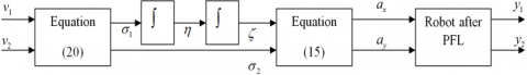
Since the sum of the dimension of the robot state $q, \dot{q}$, (i.e. 6), and the dimension of the compensator state (ξ, η), (i.e. 2), is equal to the sum of the relative degrees (4+4=8) of the two outputs defined by Eq. (21), then the input-output linearization is exactly what has been achieved. The control block diagram is given in Figure 3.
Figure 3. Scheme of the linearization controller
The advantage of using this approach is to guarantee the control of the robot while respecting the nonholonomic constraints for any time of motion T. In practice, the time of motion depends of several constraints. The next section explains in detail how to obtain it.
2.2 Off-line optimization
This section describes the method used to get the time-optimal motion T of the underactuated manipulator, from the initial position to the final desired position. The problem at hand may be mathematically formalized as: ${{\min }_{T}}\int\limits_{0}^{T}{dt}$.
Below are constraints to be considered
$\left\{ \begin{matrix} q(0)={{q}_{i}} \\ \dot{q}(0)=0 \\ \ddot{q}(0)=0 \\ \end{matrix} \right.\left\{ \begin{matrix} q(T)={{q}_{f}} \\ \dot{q}(T)=0 \\ \ddot{q}(T)=0 \\ \end{matrix} \right.$
${{M}_{pa}}{{\ddot{q}}_{a}}+{{M}_{pp}}{{\ddot{q}}_{p}}+{{C}_{p}}=0$ (22)
Geometric constraints
$\left| {{q}_{a}}(t) \right|\le {{\bar{q}}_{a,p}}$
\[\begin{matrix} \left| {{{\dot{q}}}_{a}}(t) \right|\le {{{\bar{\dot{q}}}}_{a}} \\ \left| {{{\ddot{q}}}_{a}}(t) \right|\le {{{\bar{\ddot{q}}}}_{a}} \\ \left| {{F}_{a}}(t) \right|\le {{{\bar{F}}}_{a}} \\ \end{matrix}\]
where, p and a correspond to the passive and active joints, respectively.
In order to find the optimal time, it is required to relax the nonholonomic constraint. The dynamic Eq. (22) then becomes:
${{M}_{pa}}{{\ddot{q}}_{a}}+{{M}_{pp}}{{\ddot{q}}_{p}}+{{C}_{p}}\le \varepsilon $ (23)
where, ε≤1e-3. Many algorithms may be used to find the result of this optimization problem.
The most widely used algorithms, like the genetic algorithm or the particle swarm optimization algorithm [7, 8], can converge to a global solution. The optimal time T found is then used in the method described in the previous section, to compensate for the relaxation constraint error described in Eq. (23).
To use this method with the previous one, the rest-to-rest trajectory is selected for each joint, as defined by the Eq. (24).
$q(t)={{a}_{0}}+{{a}_{1}}t+{{a}_{2}}{{t}^{2}}+{{a}_{3}}{{t}^{3}}$ (24)
Parameters a0, a1, a2 and a3 are determined from the boundary conditions; all related details are given in [9, 10].
In this section, the gravity g0=0 is considered. The purpose is to obtain the optimal control trajectory of the PPR robot manipulator $\left(\dot{x}_{s}=\dot{y}_{s}=\dot{\theta}_{s}=\dot{x}_{g}=\dot{y}_{g}=\dot{\theta}_{g}=0\right)$. Based on equations Eq. (12), Eq. (13), Eq. (16), and Eq. (18), one gets the boundary conditions for the first output y1:
$\left[ \begin{matrix} {{y}_{1s}} \\ {{{\dot{y}}}_{1s}} \\ {{{\ddot{y}}}_{1s}} \\ y_{1s}^{\left[ 3 \right]} \\ \end{matrix} \right]=\left[ \begin{matrix} {{x}_{s}}+Kc{{\theta }_{s}} \\ 0 \\ {{\xi }_{s}}c{{\theta }_{s}} \\ {{\eta }_{s}}c{{\theta }_{s}} \\ \end{matrix} \right],\left[ \begin{matrix} {{y}_{1g}} \\ {{{\dot{y}}}_{1g}} \\ {{{\ddot{y}}}_{1g}} \\ y_{1g}^{\left[ 3 \right]} \\ \end{matrix} \right]=\left[ \begin{matrix} {{x}_{g}}+Kc{{\theta }_{g}} \\ 0 \\ {{\xi }_{g}}c{{\theta }_{g}} \\ {{\eta }_{g}}c{{\theta }_{g}} \\ \end{matrix} \right]$ (25)
As for the second output, one has:
$\left[ \begin{matrix} {{y}_{2s}} \\ {{{\dot{y}}}_{2s}} \\ {{{\ddot{y}}}_{2s}} \\ y_{2s}^{\left[ 3 \right]} \\ \end{matrix} \right]=\left[ \begin{matrix} {{x}_{s}}+Ks{{\theta }_{s}} \\ 0 \\ {{\xi }_{s}}s{{\theta }_{s}} \\ {{\eta }_{s}}s{{\theta }_{s}} \\ \end{matrix} \right],\left[ \begin{matrix} {{y}_{1g}} \\ {{{\dot{y}}}_{1g}} \\ {{{\ddot{y}}}_{1g}} \\ y_{1g}^{\left[ 3 \right]} \\ \end{matrix} \right]=\left[ \begin{matrix} {{x}_{g}}+Ks{{\theta }_{g}} \\ 0 \\ {{\xi }_{g}}s{{\theta }_{g}} \\ {{\eta }_{g}}s{{\theta }_{g}} \\ \end{matrix} \right]$ (26)
To define the control input of Eq. (21), it was necessary to determine the polynomial interpolation for y1 and y2, this interpolation must satisfy the boundary conditions Eq. (25) and Eq. (26). To do this, seventh-degree polynomial Eq. (27) was used:
$\begin{align} & {{y}_{i}}={{a}_{i0}}+{{a}_{i1}}t+{{a}_{i2}}{{t}^{2}}+{{a}_{i3}}{{t}^{3}}+{{a}_{i4}}{{t}^{4}}+{{a}_{i5}}{{t}^{5}}+{{a}_{i6}}{{t}^{6}}+{{a}_{i7}}{{t}^{7}}, \\ & i=\{1,2\} \\ \end{align}$ (27)
The control vector v is the fourth derivative of y1 and y2.
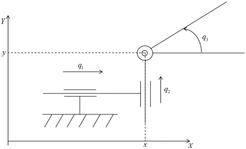
The dynamic model of the PPR manipulator robot is underactuated by the two prismatic joints [11], as shown in Figure 4.
Figure 4. PPR manipulator robot, with q1=x, q2=y and q3=θ
The model is described by the system given by the Eq. (28):
$\begin{matrix} {{m}_{x}}\ddot{x}-{{m}_{3}}l\cos \theta {{{\dot{\theta }}}^{2}}-{{m}_{3}}l\sin \theta \ddot{\theta }={{f}_{1}} \\ {{m}_{y}}\ddot{y}-{{m}_{3}}l\sin \theta {{{\dot{\theta }}}^{2}}+{{m}_{3}}l\cos \theta \ddot{\theta }={{f}_{2}} \\ I\ddot{\theta }+{{m}_{3}}l\cos \theta \ddot{y}-{{m}_{3}}l\sin \theta \ddot{x}={{f}_{3}}=0 \\ \end{matrix}$ (28)
where, l=d is the distance from the center of mass to the third axis base. To illustrate the performance of the planner, a typical result obtained for the rest-to-rest task is presented below. The manipulator robot moves from its initial position to the desired final position defined by the Eq. (29).
$\left[ \begin{matrix} {{x}_{s}} \\ {{y}_{s}} \\ {{\theta }_{s}} \\ \end{matrix} \right]=\left[ \begin{matrix} 0.5m \\ 1m \\ 0{}^\circ \\ \end{matrix} \right]\to \left[ \begin{matrix} {{x}_{g}} \\ {{y}_{g}} \\ {{\theta }_{g}} \\ \end{matrix} \right]=\left[ \begin{matrix} 1.5m \\ 2m \\ 45{}^\circ \\ \end{matrix} \right]$ (29)
here, mx=m1+m2+m3, my=m2+m3 and I=I3+m3d2 with K=2/3(l3=1m), ξs=ξg=-0.1m/s2 and ηs=ηg=0. Now, the time-optimal motion of the robot needs to be determined with the help of the method explained in Section 2.2. The results of the three optimization methods are presented in Table 1.
Table 1. Optimal time T(s)
|
SQP |
GA |
PSO |
|
21.5910 |
16.4940 |
16.3846 |
The result in Table 1 above indicates that there is no big difference between the genetic algorithm (GA) and the particle swarm optimization (PSO) algorithm, which may be explained by the fact that they both converge towards a global minimum. However, the result of the sequential quadratic programming (SQP) algorithm is higher than those of the two previous methods; this may be attributed to the initial condition of the SQP method which converges to a local minimum.
In the next step, the best optimal time value, which is given by the particle swarm optimization (PSO) approach in Table 1, is used in the method described in Section 2.1.3.
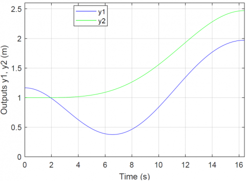
The optimal output trajectories y1 and y2 are illustrated in Figure 5 which displays the evolution of the position of the center of percussion (CP) of the last link.
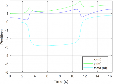
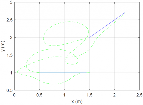
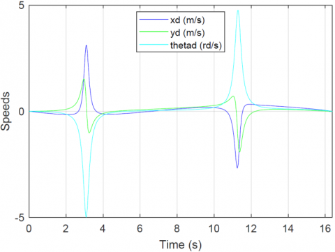
On the other hand, the evolution of generalized coordinates (x, y, θ) is depicted in Figure 6. It is worth noting that the robot starts from the initial position and arrives at the desired final position. Figure 7 shows the cartesian positions of the passive link. Here the initial and final velocities of the robot are both equal to zero, as shown in Figure 8, which means that it has an optimal rest-to-rest trajectory motion. Note also that the change in the evolution of (x, y, θ) at t=3s and t=11s corresponds to the rapid rotation of the last link near its CP as shown in Figure 6, which illustrates the cartesian positions evolution of the underactuated link.
Figure 5. Optimal output trajectories y1, y2(m)
Figure 6. Optimal positions trajectories x(m)y(m) and θ(rd)
Figure 7. Cartesian positions of the passive link
Figure 8. Optimal speed trajectories $\dot{x}(m/s), \dot{y}(m/s)$ and $\dot{\theta }(rd/s)$
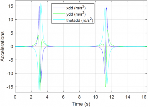
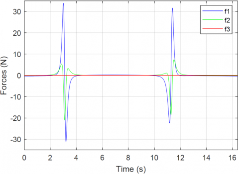
Figure 9 displays the generalized coordinates of the robot’s acceleration, and Figure 10 presents the optimal forces applied to the robot. Note that there are only the two forces f1 and f2; the last link force is equal to zero during the entire period of motion, which confirms the fact that the last link of the manipulator is underactuated. Note also that peaks in forces f1, f2 and accelerations around t=3s and t=11s correspond to the rapid rotation of the third axis near its center of percussion, which leads to a drop in the regularity index ρ.
Figure 9. Optimal acceleration trajectories $\ddot{x}\left(m / s^{2}\right), \ddot{y}\left(m / s^{2}\right)$ and $\ddot{\theta}\left(r d / s^{2}\right)$
Figure 10. Optimal forces applied to the PPR manipulator: f1, f2 and f3(N)
In the present paper, an optimal rest-to-rest trajectory was generated for an underactuated manipulator of type Xn-1Rn using a combined approach that integrates an off-line optimization that allows finding an approximate motion time using the nonholonomic constraint relaxation of the manipulator, and a relaxed error compensation using the planning trajectory method. Based on the results obtained from the combination of the two previous methods, it was possible to determine the optimal reference trajectory for controlling the Xn-1Rnmanipulator robot with n≥3.
We gratefully acknowledge the financial support from Directorate General for Scientific Research and Technological Development (la DGRSDT).
|
B |
inertia matrix |
|
C |
coriolis and centrifugal terms |
|
CP |
center of percussion |
|
dn |
the distance between the center of mass of the link n and its joint, m |
|
fx, fy |
cartesian forces, N |
|
g |
gravitational terms |
|
g0 |
gravitational acceleration, m.s-2 |
|
In |
inertia of the link n |
|
J |
jacobian |
|
k |
the forward kinematics function |
|
K |
the distance of the CP of the last link, m |
|
ln |
Length of the nth axis |
|
mn |
the mass of the link n, Kg |
|
n |
number of degrees of freedom |
|
qa |
active joint |
|
qp |
passive joint |
|
R |
rotary joint |
|
X |
any type of joints |
|
xs, xg |
starting position, goal position, m |
|
Z |
set of linear output |
|
Greek symbols |
|
|
$\eta$ |
thermal diffusivity, m2. s-1 |
|
$\theta$ |
the orientation of the last link with regard to the x-axis, rd |
|
$\sigma_{1}$ |
auxiliary input |
|
$\sigma_{2}$ |
linear acceleration, m. s-2 |
|
$\tau$ |
the torque, N m |
|
$\xi$ |
linear acceleration of the CP, m. s-2 |
[1] Choukchou-Braham, A., Cherki, B., Djemaï, M., Busawon, K. (2013). Analysis and control of underactuated mechanical systems. Springer Science & Business Media.
[2] Oriolo, G., Nakamura, Y. (1991). Control of mechanical systems with second order nonholonomic constraints: Underactuated manipulators. In IEEE Conference on Decision and Control, pp. 2398-2403. https://doi.org/10.1109/CDC.1991.261620
[3] De Luca, A., Iannitti, S., Mattone, R., Oriolo, G. (2002). Underactuated manipulators: control properties and techniques. Machine Intelligence and Robotic Control, 4(3): 113-125.
[4] Arai, H., Tachi, S. (1991). Position control of manipulator with passive joints using dynamic coupling. IEEE Transactions on Robotics and Automation, 7(4): 528-534. https://doi.org/10.1109/70.86082
[5] Arai, H., Tanie, K., Shiroma, N. (1998). Time-scaling control of an underactuated manipulator. Journal of the Robotics Society of Japan, 16(4): 561-568. https://doi.org/10.1109/ROBOT.1998.680737
[6] De Luca, A., Oriolo, G. (2002). Trajectory planning and control for planar robots with passive last joint. The International Journal of Robotics Research, 21(5-6): 575-590. https://doi.org/10.1177/027836402321261940
[7] Yang, X.S. (2010). Engineering Optimization: An Introduction with Metaheuristic Applications. John Wiley & Sons.
[8] Yang, L. (2019). An attitude motion planning algorithm for one-legged hopping robot based on spline approximation and particle swarm optimization. Revue d'Intelligence Artificielle, 33(1): 49-52. https://doi.org/10.18280/ria.330109
[9] Siciliano, B., Sciavicco, L., Villani, L., Oriolo, G. (2010). Robotics: Modelling, planning and control. Springer Science & Business Media.
[10] Zatla, H., Cherki, B., Amel, C.B. (2014). Control of an underactuated planar manipulator of RaRp type. In Proceedings of International Conference on Modeling and Simulation, pp. 136-145. https://sites.google.com/site/lesiicms/proceedings.
[11] Imura, J.I., Kobayashi, K., Yoshikawa, T. (1996). Nonholonomic control of 3 link planar manipulator with a free joint. In Proceedings of 35th IEEE Conference on Decision and Control, Kobe, Japan, pp. 1435-1436. https://doi.org/10.1109/CDC.1996.572714