Giulio Lorenzini | Mehrdad Ahmadi Kamarposhti* | Ahmed Amin Ahmed Solyman
© 2021 IIETA. This article is published by IIETA and is licensed under the CC BY 4.0 license (http://creativecommons.org/licenses/by/4.0/).
OPEN ACCESS
Tracking maximum power in photovoltaic applications is considered a major issue. Because of the change in the output power of solar cells by changing the radiation and temperature, it is required to receive the maximum power from solar array to be achieved the maximum efficiency using maximum power tracking methods. A large number of the maximum power methods have been introduced so far, but each has difficulty in terms of tracking speed and accuracy, and in practice, they have not been able to improve both of these factors. Among the commonly used methods, the incremental conductance method has a good tracking speed and accuracy, but at the same time, it cannot reach both to a desirable value. In this paper, a new method is proposed based on the above method that improves the mentioned factors simultaneously to an acceptable limit. The result of the simulation confirms the correctness of the claim of the proposed method.
solar cell, photovoltaic system, maximum power tracking, incremental conductance algorithm
Photovoltaic PV has been used in recent years as a reliable, pure and unlimited source of energy. The high cost of initial setting up and low efficiency of energy conversion are among the disadvantages of using photovoltaic systems. To reduce the disadvantages, many efforts are being made to increase the efficiency of energy conversion by increasing the quality of solar cells and receiving the maximum power of solar cells. Characteristics of photovoltaic systems are inherently nonlinear and are subject to environmental parameters such as radiation, ambient temperature and load connected to it. Therefore, by proper choosing of the work point of PV array, it can be received the maximum power from the PV array under constant radiation and temperature conditions. By the changes in the environmental conditions (radiation and temperature), the array's work point is changed, and as a result, using different algorithms of maximum power point tracking, it can be kept the amount of power received from the array at its maximum, in other words, traced the maximum power point.
There are various ways for maximum power tracking. The main methods are Hill-Climbing, Perturb & Observe, incremental conductance, fuzzy logic control, parasitic capacitance, control dependent on ripple ... In these methods, solar arrays have been fixed, therefore, by moving the sun and changing the angle of radiation on the surface of the solar arrays, the power received from the PV array is reduced, but again in this case, under different environmental conditions, extraction of the maximum power from the PV array is important. By using the maximum power tracking system, the system is always set in a mode that always has the highest power independent of environmental conditions or load conditions [1, 2].
So far, several methods have been proposed and used for maximum power tracking that some of these methods are introduced. One of the most commonly used power tracking methods is the perturbation and observation (P & O) method. This technique is used to track the maximum power point [3]. In this method, the reference of the solar panel can be implemented by applying disturbances to the signal of reference voltage or current signal. In this algorithm, if the reference signal X is a voltage (i.e, X = V), the target, contains reference voltage signal to the VMPP, so it causes to follow the VMPP's instantaneous voltage. As a result, the output power will reach MPP. The conductance method is similar to the P & O method, but based on the sum of the ratio of the current to the voltage and their derivative ratio, this value is zero at the maximum power point [4, 5]. The reference [6] applies an incremental conductance method specifically for solving the power-tracking problem. To increase the speed and accuracy of incremental conductance methods with variable steps that change dynamically by changing input conditions. In this paper, a system based on the incremental conductance method is presented that done the rapid and accurate tracking of maximum power point, and then by setting a DC-to-DC converter delivers the most power to load.
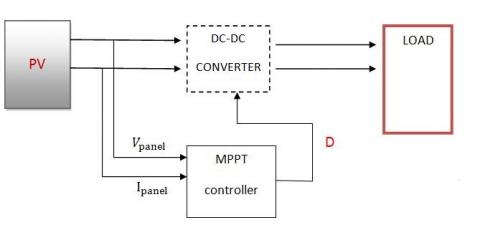
In order to implement a system that has the ability to trace the maximum power point, it is necessary for the system to contain components including array of PV, DC-to-DC converter and a programmable controller for applying MPPT algorithms. The overall structure of a PV system is shown in Figure 1.
Figure 1. The general structure of a photovoltaic system [3]
2.1 Characteristics of the photovoltaic array
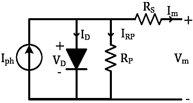
A photovoltaic array is composed of series and parallel sets of solar cells. Each solar cell is an N-P link whose electrical equivalent circuit is shown in figure. The Iph current source represents the effect of the optical current. Eq. (1) shows RS series resistance, the internal resistance of the cell against flow passage and the parallel resistance Rp represents the leakage currents. Of course, the equivalent circuit of Figure 2 can also be used for modules or photovoltaic arrays [7-9].
Figure 2. Equivalent electrical circuit of a cell or photovoltaic module [6]
Im=Iph-ID-IRp (1)
where,
Iph is the current of radiation light, (which it depends directly on the amount of sun radiation).
ID: Current of the direct connection of diode.
IRp: Current flowing from the parallel resistance.
The output current of the PV array is obtained by Eq. (2):
Im=NpIph-NpIrs$\left[\mathrm{e} \frac{q(v+R_{S} I_{O})}{A K T N_{S}}-1\right]-\mathrm{N}_{\mathrm{p}} \frac{q(v+R_{S} I_{O})}{N_{S} R_{R_{p}}} \mathrm{I}_{\mathrm{o}}$ (2)
where,
Im: PV Array output current PV.
K: Boltzmann constant.
Irs: cell reverse saturation current.
T: Temperature (in terms of Kelvin).
q: Electron charge.
A: P-N quality factor.
Ns and Np, respectively, are the number of connected cells in series and in parallel.
The radiation current Iph depends on the amount of radiation and temperature obtained from the equation below:
$\mathrm{I}_{\mathrm{ph}}=\frac{G}{1000}\left(\mathrm{I}_{\mathrm{SC}}+\mathrm{k}_{\mathrm{i}}\left(\mathrm{T}-\mathrm{T}_{\mathrm{r}}\right)\right)$ (3)
where:
Isc: Short-circuit current of cell at temperature and reference radiation.
Tr: Cell reference temperature.
Ki: Temperature coefficient of short-circuit current.
G: Sun radiation in terms of w/m2.
In addition, the reverse saturation current is calculated from the following equation:
$\mathrm{I}_{\mathrm{rs}}=\mathrm{I}_{\mathrm{rr}}\left[\frac{T}{T_{r}}\right]^{3} \exp \left(\frac{\mathrm{q}. \mathrm{E}_{\mathrm{G}}}{\mathrm{k} . \mathrm{A}}\left(\frac{1}{T_{r}}-\frac{1}{T}\right)\right)$ (4)
where:
Irr: Reverse saturation current in Tr.
EG: band gap energy of the semiconductor used in the cell.
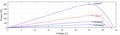
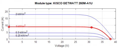
Figures 3 and 4 and P-V and I-V specifications of the PV cell used in this paper, which is the KISCO GETWATT 26M-A1U model, is shown in terms of radiation and temperature values. Details of this model are presented in the simulation section.
Figure 3. Voltage-power diagram of the photovoltaic module for radiation values (0.25-0.5-1-2) (kw / m2)
Figure 4. Current-voltage diagram of the photovoltaic module for radiation values (0.25-0.5-1-2) (kw / m2)
Output voltage of PV arrays with series-parallel connection structure is relatively low. Therefore, high-efficiency incremental DC-DC converters need to convert the low voltage of PV arrays to high voltage as 380 V for full bridge converters or 760 V for half-bridge converters in 220 V networks. Conventional boost converters are widely used in renewable energy applications due to simple orbital structure. In Figure 5, a single-phase boost converter and single-switch are shown [10].
In order to match the load with the PV array in order to absorb the maximum power, the switching converter is used as a power processor, which is a voltage incremental converter and the output voltage level is controlled by the setting of the switching. Today, modern converters have high power density and high switching frequency, which reduces the size of these converters. To achieve this goal, soft switching techniques should be used.
Figure 5. Simple boost converter [11]
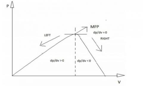
The incremental conductance method uses the slope of power characteristics of PV array to track MPP. This method is based on the fact that the slope of curve of the array PV determines the position of the array's work point of to the MPP point [12]. By the presentation of Figure 6, the method of incremental conductance will be explained more precisely. According to Figure 6, it can be said that the slope of the above curve at the maximum power point is equal to zero, that slope of curve increases on the left side, and the curve slope decreases on the right side. Therefore, the basic equations of the incremental inductance method will be as follows.
At MPP Point, according to the critical point:
$\frac{d P}{d V}=0$ (5)
Eq. (5) can be rewritten as follows:
$\frac{d P}{d V}=\frac{d(V I)}{d V}=I+V \frac{d I}{d V}=0-->\frac{d I}{d V}=-\frac{I}{V}$ (6)
Therefore, at the MPP point, Eq. (6) will be established.
At the maximum power point,
$\frac{d I}{d V}=-\frac{I}{V}$ (7)
The left side of the maximum power point,
$\frac{d I}{d V}>-\frac{I}{V}$ (8)
The right side of the maximum power point,
$\frac{d I}{d V}<-\frac{I}{V}$ (9)
Due to the above, it is possible to create an algorithm that leads to the acquisition of maximum power from the photovoltaic cell. In this algorithm, the voltage and output current of the photovoltaic cell are measured at each instant and, according to (7) to (9), the value of D (duty cycle) is determined. Flowchart of incremental conductivity method is shown in Figure 7 [13, 14].
Figure 6. Various areas of panel PV function
As shown in Figure 7, the output signal under control in the D incremental conductance algorithm is converted to a comparator block and the final output of the command pulses to the MOSFET gate is applied to the converter.
As it is shown in the algorithm of Figure 7, this algorithm is only dependent on the local position of the array's work point to the MPP point, regardless of the distance to the MPP point, adds or detracts a constant amount of ($\Delta D$) from D. Naturally, the low value of $\Delta D$ will reduce the tracking rate and also the increase of its amount causes the fluctuations around the MPP point [12].
Figure 7. Normal incremental conductivity method algorithm [15]
Research in the field of tracking power point under methods of variable step length is begun since 2008, and newer methods are being replaced previous methods each day. The principle idea of all these methods that are based on the incremental conductivity method is the same and the difference between these methods is in how to include variable steps in this algorithm or converter used for system modeling [16]. Table 1 summarizes these methods and compares them with each other.
Table 1. MPP control incremental conductivity methods with variable step length
|
Reference |
Year |
Author |
Step of variable |
Converter DC-DC |
Explanations |
|
[12] |
2008 |
Liu et al. |
D(K)=D(K-1)±N| $\frac{d p}{d v}$ | |
Push-pull |
Proper dynamic Middle speed of tracking Without fluctuations of steady state High overshoot |
|
[14] |
2011 |
Mei et al. |
$\mathrm{C}=P^{n} *|d p / d i|$ |
Boost |
Proper dynamic Without fluctuations of steady state Middle speed of tracking High overshoot |
|
[16] |
2011 |
Ahmed Emad |
C= $\frac{d v}{d i}+\frac{v}{i}$ |
Boost |
High fluctuations in steady state High overshoot |
|
[15] |
2013 |
Rahman et al. |
D(K)= $\frac{d V}{d I}+\frac{V}{I}$ |
Buck |
Low speed of tracking High fluctuations of fix state |
|
[11] |
2014 |
Tey and Mekhilef |
Step=N* $\frac{d p}{d v}$ |
Sepic |
Proper dynamic Without fluctuations of fix state High overshoot |
|
[17] |
2014 |
Abdourraziq et al. |
D(K)=D(K-1)±N| $\frac{d p}{d v}$ | |
Boost |
Speed of high response Ripple of high voltage High overshoot |
The proposed algorithm in this paper is based on the same method of incremental conductance, but the length of its variable steps depends entirely on the dynamic state of the system. The step length is defined as follows:
$S T E P=[D(K)-D(K-1)] *\left|\frac{d P}{d V-d I}\right|$ (10)
In this case, the variations of power are not only dependent on the amount of power variations to the voltage, but also the variations are relative to the difference in voltage and current variations. In addition, in the past, the constant number was used as a coefficient, while in this method, for different working conditions, coefficient will be different, i.e. both the first part and the second part depend on the position of the work point. The algorithm of the proposed method is shown in Figure 8.
Now calculate the converter values. The equations related to the calculation of the incremental converter parameters are as follows [18]:
$V_{o u t}=\frac{\text { Vin }}{1-D}$ (11)
$L=\frac{D \times V_{i n}}{f_{s w} \times \delta_{I} \times I_{L}}$ (12)
$C=\frac{I_{o u t} \times D}{f \times \delta_{V} \times V_{o u t}}$ (13)
Regarding the voltage at maximum power, this voltage is selected as the input voltage and the output voltage is considered to be 70 V.
D=0.56, L=685 $\mu H$ and C=295 $\mu F$
In order to investigate the accuracy and efficiency of the proposed method, a photovoltaic system consisting of a solar array, a DC-DC boost converter, and a control system (MPP detector) are simulated in the MATLAB/Simulink environment. In order to compare the results of the proposed method with other methods under the same conditions, the same equipment and elements in the photovoltaic panel and converter parts will be used. For this purpose, various simulations and tests have been used on the common array model in MATLAB (KISCO GETWATT 260M-A1U), which is described in Table 2.
Table 2. Specifications of Photovoltaic Module
|
Maximum power |
260 V |
|
Maximum voltage |
31 V |
|
Maximum current |
8.4 A |
|
Short circuit current |
8.8 A |
|
Open circuit voltage |
38.1 V |
|
Current temperature coefficient |
(0.042898) %/℃ |
|
Voltage temperature coefficient |
-(0.36441) %/℃ |
|
The effect of temperature on power |
-(0.5$\pm$0.5) %/℃ |
Considering standard conditions, simulation using different controllers is done. As follows, the performance of incremental conductance algorithm with variable step length in improving the output power of the photovoltaic module will be compared and assessed with the observation algorithm or the normal incremental conductance algorithm.
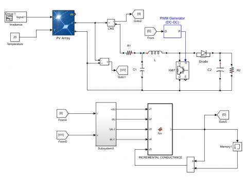
In Figure 8, the overview of the simulated system is shown. As shown in this figure, the system consists of three general sections, the first part of which is the array or photovoltaic module, the specifications of which are presented in this chapter, and the inputs of this section are radiation and temperature signals, and the output will be a DC voltage, which is the output voltage of array. The second part of the system is the boost incremental DC-DC converter, which accepts the voltage of output DC of the array, and delivers the desired output voltage to load with orbital operation which done on the voltage level.
The third part of the system that this thesis is focused on it is the control section of output voltage by setting the duty cycle. In this section, the voltage and current signals are sampled and monitored from the input of the array. These values are recorded and entered into a control cycle. Finally, the output of this section is transmitted as the basis for adjusting the duty cycle to the pulse generator modulator.
In order to evaluate and confirm the performance of the proposed method and compare it with ordinary MPPT methods in terms of efficiency, dynamics, accuracy and speed, the performance of different tests is performed on the algorithms and the results are presented in the form of the following.
As calculated from the numerical results of Figure 9, the efficiency of the proposed method is about 96% which is relatively higher compared to similar algorithms.
Given the output power of the array and the output power of the converter, the efficiency will be calculated from the following equation:
$\eta=\frac{\text { Parray }}{\text { Pconv }}$ (14)
The cases that have been improved during the proposed algorithm include tracking accuracy, response time and fluctuations. In the following, each of these cases will be discussed and compared in detail for the proposed algorithm and the normal incremental conductance algorithm. The performance of output power of fixed step length method (normal incremental conductance), variable step length method (proposed algorithm) is shown under the conditions of change in the radiation level in the following Figures. Table 3 shows comparison of the efficiency of the proposed method and other common methods.
Figure 8. The general system simulated in MATLAB software
Figure 9. The difference between array output power and converter output power
Table 3. Comparison of the efficiency of the proposed method and other common methods
|
|
Method |
Efficiency |
|
1 |
P&O |
92% |
|
2 |
Conventional incremental conductance |
92% |
|
3 |
Proposed algorithm |
96% |
6.1 MPP tracking
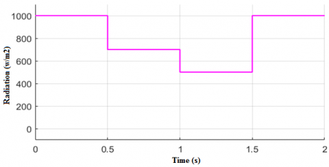
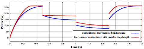
Figure 12 shows MPPT methods of incremental conductance with a fixed step length and variable step length related to the input of radiation levels (1000-700-500w/m) where we can observe and compare the two comparison algorithms in this article.
Figure 10 shows the relevant radiation. As shown in Figure 11, for sudden changes in the level of radiation, the normal algorithm will be gone away from the tracking path and will result in power losses (on average 20 watts), which this amount of power will be the amount of energy in long-term that will be wasted.
Figure 10. Radiation Signal (1000-700-500 w/m)
Figure 11. Comparison of MPP tracking of fixed step length method and variable step length
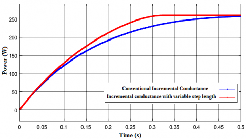
6.2 Response time
Comparison of MPPT methods with the size of the fixed step length and the variable step length are shown again in Figure 11 from another aspect. The proposed algorithm shows a significant improvement during response time, so the energy losses by the proposed algorithm can be reduced. As shown in Figure 12, the time difference in convergence to the final value in the proposed algorithm is improved approximately 0.2 seconds compared to the normal algorithm.
Figure 12. Comparison of the response time to reach the MPP point of the fixed step length method and the variable step length
6.3 Continuous changes of radiation
In the cases that radiation changes are continuous and sinusoidal, the normal algorithm has a lower accuracy than the proposed algorithm. Figure 13 shows the relevant radiation. The result of this test is shown in Figure 14 by applying radiation signal.
According to the results of this test, the difference between the system output powers for sinusoidal changes of radiation will be an average of 10 watts, which will be improved by the proposed algorithm.
Table 4 presents a brief overview of the normal and proposed methods. As it can be seen in this table, the algorithm not only has fluctuations of low steady state but also, in some cases, the speed of reaching MPP, the algorithm's dynamics and the efficiency of the proposed algorithm follows more suitable results than other common methods.
Figure 13. Continuous changes of radiation
Figure 14. Comparison of the output power of the system for sinusoidal changes of radiation
Table 4. General comparison of the proposed method with other common methods
|
Method |
Efficiency |
Dynamics |
Steady state fluctuations |
Overshoot |
Speed to reach MPP |
|
P&O |
$\cong$0.93 |
Medium |
Low |
Low |
$\cong$0.5 s |
|
Incremental conductivity |
$\cong$0.92 |
Medium |
Low |
Low |
$\cong$0.5 s |
|
Method |
$\cong$0.97 |
Good |
Low |
Low |
$\cong$0.3 s |
In this paper, an improved method for incremental conductance MPPT algorithm with variable step length is presented. First, incremental conductivity method was specifically expressed and based on the weaknesses in this method, and the modified methods for this algorithm, the proposed proposal was discussed in detail. A comparative study was shown between the incremental conductance MPPT method with fixed step length and variable step length under the same operating conditions and with the application of different radiation signals. Simulation results show that using an incremental conductance algorithm with variable step length, there is a significant improvement over the steady state function, the dynamic response to the system as well as the response time to the system. Due to the practical application of this system and the life of photovoltaic systems, a little amount in the improvement of performance and efficiency of these systems will compensate a large amount of energy losses. Therefore, an incremental conductance MPPT algorithm with variable step length is a good justification for the modification of normal method and has a larger contribution to remove noise, turbulence and energy reduction.
[1] Subudhi, B., Pradhan, R. (2013). A comparative study on maximum power point tracking techniques for photovoltaic power systems. IEEE Transactions on Sustainable Energy, 4(1): 89-98. http://dx.doi.org/10.1109/TSTE.2012.2202294
[2] Reisi, A.R., Moradi, M.H., Jamas, S. (2013). Classification and comparison of maximum power point tracking techniques for photovoltaic system: A review. Renewable and Sustainable Energy Reviews, 19: 433-443. http://dx.doi.org/10.1016/j.rser.2012.11.052
[3] Liu, F.R., Kang, Y., Zhang, Y., Duan, S.X. (2008). Comparison of P&O and hill climbing MPPT methods for grid-connected PV converter. 3rd IEEE Conference on Industrial Electronics and Applications. http://dx.doi.org/10.1109/ICIEA.2008.4582626
[4] Liu, B.Y., Duan, S.X., Liu, F., Xu, P.W. (2007). Analysis and improvement of maximum power point tracking algorithm base on incremental conductance method for photovoltaic array. 7th International Conference on Power Electronics and Drive Systems, pp. 637-641. http://dx.doi.org/10.1109/PEDS.2007.4487768
[5] Arulmurugan, R., Suthanthira Vanitha, N. (2013). Numerical analysis of incremental conductance with cyclic measurement of the MPPT algorithm for PV power generation. IET Chennai Fourth International Conference on Sustainable Energy and Intelligent Systems. http://dx.doi.org/10.1049/ic.2013.0297
[6] Lee, J.H., Bae, H., Cho, B.H. (2006). Advanced incremental conductance mppt algorithm with a variable step size. 12th International Power Electronics and Motion Control Conference, pp. 603-607. http://dx.doi.org/10.1109/EPEPEMC.2006.4778466
[7] Nakanishi, F., Ikegami, T., Ebihara, K., Kuriyama, S., Shiota, Y. (2000). Modeling and operation of a 10 kW photovoltaic power generator using equivalent electric circuit method. Conference Record of the Twenty-Eighth IEEE Photovoltaic Specialists Conference, pp. 1703-1706. http://dx.doi.org/10.1109/PVSC.2000.916231
[8] Salas, V., Olias, E., Barrado, A., Lazaro, A. (2006). Review of the maximum power point tracking algorithms for stand- alone photovoltaic systems. Solar Energy Mater. Solar Cells, 90(11): 1555-1578. http://dx.doi.org/10.1016/j.solmat.2005.10.023
[9] Khaligh, A., Onar, O.C. (2010). Solar, wind, and ocean energy conversion systems. Energy Harvesting, Taylor and Francis Group, LLC, 23-53. https://dx.doi.org/10.1201/9781439815090
[10] Piegari, L., Rizzo, R. (2010). Adaptive perturb and observe algorithm for photovoltaic maximum power point tracking. IET Renewable Power Generation, 4(4): 317-328. https://dx.doi.org/10.1049/iet-rpg.2009.0006
[11] Tey, K.S., Mekhilef, S. (2014). Modified incremental conductance MPPT algorithm to mitigate inaccurate responses under fast-changing solar irradiation level. Sol Energy, 101: 333-342. https://doi.org/10.1016/j.solener.2014.01.003
[12] Liu, F., Duan, S., Liu, F., Liu, B., Kang, Y. (2008). A variable step size INC MPPT method for PV systems. IEEE Transactions on Industrial Electronics, 55(7): 2622-2628. https://doi.org/10.1109/TIE.2008.920550
[13] Abdourraziq, M.A., Maaroufi, M., Ouassaid, M. (2014). A new variable step size INC MPPT method for PV systems. International Conference on Multimedia Computing and Systems. http://dx.doi.org/10.1109/ICMCS.2014.6911212
[14] Mei, Q., Shan, M., Liu, L., Guerrero, J. (2011). A novel improved variable step size incremental resistance MPPT method for PV systems. IEEE Trans Indus Electron, 58(6): 2424-2434. http://dx.doi.org/10.1109/TIE.2010.2064275
[15] Abdul Rahman, N.H., Omar, A.M., Mat Saat, E.H. (2013). A modification of variable step size INC MPPT in PV system. In: Proceedings of the 7th IEEE International Power Engineering and Optimization Conference (PEOCO), pp. 340-345. http://dx.doi.org/10.1109/PEOCO.2013.6564569
[16] Ahmed, E.M., Shoyama, M. (2011). Stability study of variable step size incremental conductance/impedance MPPT for PV systems. In: Proceedings of the 8th International Conference on Power Electronics - ECCE Asia, pp. 386-392. http://dx.doi.org/10.1109/ICPE.2011.5944555
[17] Abdourraziq, M.A., Maaroufi, M., Ouassaid, M. (2014). Comparative study of MPPT using variable step size for photovoltaic systems, Comparative study of MPPT using variable step size for photovoltaic systems. In: Proceedings of the Second World Conference on Complex Systems (WCCS) Agadir, Morocco, pp. 374-379. http://dx.doi.org/10.1109/ICoCS.2014.7060939
[18] Ferchichi, M., Zaidi, N., Khedher, A. (2016). Comparative analysis for various control strategies based MPPT technique of photovoltaic system using DC-DC boost converter. 17th International Conference on Sciences and Techniques of Automatic Control and Computer Engineering (STA), pp. 27-41. http://dx.doi.org/10.1109/STA.2016.7951990