Aicha Hachana* | Mohamed Naguib Harmas | Ziyad Bouchama
© 2021 IIETA. This article is published by IIETA and is licensed under the CC BY 4.0 license (http://creativecommons.org/licenses/by/4.0/).
OPEN ACCESS
Blood glucose automatic regulation achievement depends on the robustness of the used control algorithm. However, some constraints were encountered due to the human glucose-insulin regulatory system’s complexity. It is proposed to tackle such a goal through the development of a robust synergetic control algorithm. An adaptive approach is integrated into this synergetic control scheme to handle disturbances and parameters variations. Multiple meal disturbances often occur daily as well as some other stochastic noises making efficient glucose regulation a tough challenge addressed in this paper via a new synergetic scheme. Simulation results show a robust function during multiple meal disturbances with good noise rejection.
synergetic control, adaptive systems, uncertain system, glucose regulation
Diabetes mellitus can be described as a chronic illness occurring upon insulin production deficiency by the pancreas, or by the feebleness of the insulin produced. Such a serious condition covers a group of metabolic sicknesses during an extended period of high blood sugar levels, which in turn harm many of the body's systems, especially, blood vessels, and nerves.
A well-known way to treat patients consists in an injection of insulin very often self-administrated. There are various devices used to inject insulin, syringes, pumps, patches, etc... A main concern with this therapeutic approach is that the insulin injection is to be controlled by the patient himself. An ideal solution to this issue would be to create a treatment type such that this burden is alleviated on the patient and that the insulation injections take place automatically whenever needed. Thus, this can be realized in a self-regulated pump functioning as an artificial pancreas [1]. Besides, due to glucose–insulin regulatory system time variation and nonlinear control, the patient’s parameters’ detection is costly, invasive and undergoes a number of uncertainties.
For instance, insulin resistance levels can vary with regular exercising [1], i.e., muscle mass intakes glucose with no insulin intervention. The blood glucose’s scope of operation of a diabetic is large, and can differ between 45 and 500 mg/dl.
With these constraints, applying linear control to regulate blood glucose using automated insulin injection has become difficult. Some of these algorithms such as classical methods PID [2], proportional-derivative (PD) [3], and latter optimal control algorithms [4], the H∞ controller [5] and MPC algorithms [6] have been used through linearized model.
In this research, synergetic control [7] is used in the control algorithm design for the regulatory system of glucose-insulin. Moreover, synergetic control is an effective nonlinear robust technique. Hence, similar to sliding mode methodology [8], a closed loop system dynamic is provided, i.e., constancy to uncertainties as well as correctness and strength, which are also the properties of synergetic control [9]. Therefore, these properties are consistent with the human control algorithm specifications, where accuracy is of a paramount importance. Notably, the glucose metabolism’s sophisticated nonlinear system is due to several factors, often immeasurable, such as food intake quantity; thus, parameter measurements vary from patient to patient, besides other activity conditions which make an appropriate adaptive control technique. However, the suggested control regulations have to be adapted to overcome the fact that the controlled system parameters can vary over time or doubtful. Furthermore, the adopted control involves improving dynamic system properties, whereas the controlled environment or plant specifications are unstable [10]. In order to assure system constancy and assign a tracking point even in presence of unknown boundary disturbances, a new adaptive estimation method is integrated into the synergistic scheme used.
A new adaptive law utilizing the concept of terminal attractor is put to use in the procedure of finite time control of nonlinear systems; this ensures a faster parameters adaptation procedure which results in an improvement of closed loop overall robustness.
Next, a review on glucose-insulin system modeling in type I diabetic mellitus is introduced, and then a brief presentation covering synergetic control design in section III is presented. After that, the adaptive synergetic control is investigated in section IV. Finally, section V presents simulation results followed by a conclusion as a conclusive section.
Several glucose-insulin process examples were suggested; for instance, Bergman minimal model developed in 1980 by Richard Bergman. Besides, the interaction between main system components such as glucose and insulin concentrations is appropriately presented without plunging into human biological complexity. The principal advantage of the Bergman minimal model lies in the minimum number of parameters involved. The Bergman minimal model [11, 12] is given in (1):
$G(t)=-{{p}_{1}}\left[ G(t)-{{G}_{b}} \right]-X(t)G(t)+D(t)$
$X(t)=-{{p}_{2}}X(t)+{{p}_{3}}\left[ I(t)-{{I}_{b}} \right]$
$I(t)=-n\left[ I(t)-{{I}_{b}} \right]+\gamma {{\left[ G(t)-h \right]}^{+}}t+u(t)$ (1)
where, G(t), X(t) and I(t) are plasma glucose concentration (mg/dl). Thus, the insulin reduction effect on glucose concentration and insulin concentration level in plasma is measured by (μU/ml). Besides, Ib is the basal blood insulin, and Gb represents the basal glucose concentrations. Moreover, γ is for the pancreatic β- cells’ rate that release insulin after glucose insertion and formulated as [(µU/ml min-2 (mg/dl)-1]. Yet, h is the above glucose sill value in which the pancreatic β- cells release insulin (mg/dl), and n measure of insulin consumed in plasma (1/min). Additionally, u(t) is the insulin dose rate (μU/ml) is the controller and replaces the normal insulin regulatory system of the body, which does not exist in diabetic patients. The [G(t)-h]+t equation represents the pancreatic insulin release after food intake at t=0, which is not the case for patients with diabetes [12].
D(t) represents a disturbance indicator; it can be exemplified by a decaying exponential function as such:
$D(t)=A{{e}^{(-Bt)}},B>0$ (2)
in which, D (t) is represented by (mg/dl/min).
•The exponential form phrase γ exp (−0.05t) represents moderate meals state [13].
•The exponential form phrase ε exp (−0.025t) represents significant unsystematic effects because of factors such as exercising [13]. The first equation of (1), describes the dynamics of glucose metabolism. The second equation of (1) represents the dynamics of insulin transport from the blood to the interstitial fluid. The last equation of (1) describes the change in insulin concentration in the blood over time.
Synergetic control is an effective nonlinear control technique similar to sliding mode control; however, not including chattering. Stabilizing the glucose concentration in the diabetic patient’s blood at the basal level Gb is an output-tracking problem thus, the tracking error is defined:
$e={{G}_{b}}-G$ (3)
The system presented in Eq. (1) is non-linear can be reformulated in state-space realm as such;
${{x}_{1}}=-{{p}_{1}}\left[ {{x}_{1}}-{{G}_{b}} \right]-{{x}_{1}}{{x}_{2}}+D(t)$
${{x}_{2}}=-{{p}_{2}}{{x}_{2}}+{{p}_{3}}\left[ {{x}_{3}}-{{I}_{b}} \right]$
${{x}_{3}}=-n\left[ {{x}_{3}}-{{I}_{b}} \right]+\gamma {{\left[ {{x}_{1}}-h \right]}^{+}}t+u(t)$ (4)
where, x1, x2and x3 are G(t), X(t) and I(t), respectively. Then, the observed error is reformulated as:
$e={{G}_{b}}-G={{G}_{b}}-{{x}_{1}}$ (5)
Firstly, the system relative degree must be determined, assuming y=x1and using Eq. (5), by the successive differentiations’ number until control function appears [14]. The latter appears the third differentiation, i.e.:
$x_{1}^{(3)}=\varphi (x,t)-{{p}_{3}}{{x}_{1}}u(t)$. (6)
where,
$\begin{align} & \varphi (x,t)={{x}_{1}}\left[ -{{p}_{1}}(p_{1}^{2}+3{{p}_{3}}{{I}_{b}})-{{p}_{3}}{{I}_{b}}({{p}_{2}}+n)-{{p}_{3}}\gamma {{({{x}_{1}}-h)}^{+}}t \right] \\ & +{{x}_{2}}\left[ -p_{1}^{2}(1+{{G}_{b}})+{{p}_{1}}{{p}_{2}}(2{{G}_{b}}-1)+2D({{p}_{1}}+{{p}_{2}}) \right] \\ & +{{x}_{3}}\left[ -2{{p}_{3}}({{p}_{1}}+D) \right]+{{x}_{1}}{{x}_{2}}\left[ -{{({{p}_{1}}+{{p}_{2}})}^{2}}-3{{p}_{3}}{{I}_{b}} \right] \\ & +{{x}_{1}}{{x}_{3}}\left[ {{p}_{3}}\left( 3{{p}_{1}}+{{p}_{2}}+n \right) \right]+{{x}_{1}}x_{1}^{2}\left[ -3{{\left( {{p}_{1}}+{{p}_{2}} \right)}_{{}}} \right] \\ & +x_{2}^{2}\left( {{p}_{1}}{{G}_{b}}+D \right)+3{{p}_{3}}{{x}_{1}}{{x}_{2}}{{x}_{3}}-{{x}_{1}}x_{2}^{3}+D \\ & +\left( {{p}_{1}}{{G}_{b}}+D \right)\left( p_{1}^{2}+2{{p}_{3}}{{I}_{b}} \right) \\ \end{align}$
Letting the macro-variable be chosen as:
$\psi=e+c_{1} e+c_{0} e$ (7)
To develop the control, the system must be forced to work on the manifold:
$\psi =0$ (8)
The designer may select properties of this macro variable according to the suggested control specifications. Hence, a macro variable simple selection would be in an inconsistent linear combination state. The required dynamic evolution of the macro variables can be selected as:
$T \psi+\psi=0$ (9)
where, T is a device parameter determining the conflux speeds to the manifold (9).
Then, instantly substituting (7) and (9) into (3) and readjusting, the obtained control law is given by
$u=\frac{1}{{{p}_{3}}{{x}_{1}}}(-\frac{\psi }{T}+\varphi -{{c}_{1}}{e}+{{c}_{0}}e)$ (10)
Since p3≠0, x1≠ 0, and p3x1 [1.2×10−4,3×10−2], and c1 and c0 are invariants real-valued.
The elaborated control assures an asymptotic convergence until the final state. Asymptotic constancy is derived by selecting the candidate Lyapounov function:
$V=\frac{1}{2}\psi {{(e)}^{2}}$ (11)
After differentiation, it leads to:
$\dot{V}=\psi(e) \dot{\psi}(e)$
$\dot{V}=\psi(e)\left(\dddot e+c_{1} \ddot{e}+c_{0} \dot{e}\right)=\psi(e)\left(-\ddot{x}_{1}+c_{1} \ddot{e}+c_{0} \dot{e}\right)$ (12)
$\dot{V}=\psi (e)\left( -\varphi +{{p}_{3}}{{x}_{1}}u+{{c}_{1}}\ddot{e}+{{c}_{0}}\dot{e} \right)$ (13)
Then, replacing (10) by (13):
$\dot{V}=\psi (e)\left( -\frac{1}{T}\psi (e) \right)=-\frac{1}{T}\psi {{(e)}^{2}}$ (14)
Thus, the controller can reach Lyapunov constancy.
An adaptive estimation to disturbance is implemented to free the control system from the boundary values’ disturbance, and then the synergetic controller would be adjusted.
Let estimate error to be determined as:
${{e}_{F}}=F-\hat{F}$ (15)
in which, $\widehat{F}$ is the estimated value of F. Here, a law adaptation is suggested using the concept of a fast terminal technique, that is the research aim, so as the estimated error is zero indefinitely.
Theorem 1
If the estimated disturbance is adjusted by:
$\hat{F}=(\alpha {{e}_{F}}+\beta e_{F}^{{}^{q}/{}_{p}})$ (16)
where:
$\alpha>0, \beta>0$, with $p>q>0$ odd integers.
Then we can conclude that:
The estimated disturbance will remain bounded. The estimated error eF will definitely reach zero.
Proof. Suggesting the candidate Lyapunov function to be:
${{V}_{F}}=\frac{1}{2}{{e}_{F}}^{2}$ (17)
Therefore,
$\begin{align} & {{{\dot{V}}}_{F}}={{e}_{F}}{{{\dot{e}}}_{F}}={{e}_{F}}(-\hat{F})=-{{e}_{F}}(\alpha {{e}_{F}}+\beta e_{F}^{{}^{q}/{}_{p}}) \\ & =-\alpha e_{F}^{2}-\beta e_{F}^{{}^{(p+q)}/{}_{p}})=-\alpha {{V}_{F}}-\beta V_{F}^{{}^{(p+q)}/{}_{p}} \\ \end{align}$ (18)
Thus, we have $\dot{V}_{F} \leq 0$ for all $V_{F} \geq 0$ and will be asymptotically convergent, because $0<\frac{p+q}{2 p}<1$, therefore, the estimated parameter disturbance will remain bounded.
Lemma 1: If a Lyapunov function is expressed as:
$\dot{V}(t)+a'V(t)+{b}'{{V}^{\eta }}(t)\le 0,\forall t\ge {{t}_{0}},V({{t}_{0}})\ge 0$ (19)
where, $a, b>0,0<\eta<1$.
Finite time is given by the following expression:
$t=\frac{1}{{\alpha }'(1-\eta )}\ln (\frac{{\alpha }'V{{(0)}^{1-\eta }}+{\beta }'}{{{\beta }'}})$ (20)
From lemma 1 in [15], (18) can be written as:
${{\dot{V}}_{F}}+\alpha {{V}_{F}}+\beta V_{F}^{{}^{(p+q)}/{}_{2p}}\le 0$ (21)
Thus, the estimation error converges to zero in finite time given by:
$t=\frac{1}{\alpha (1-\frac{q+p}{2p})}\ln (\frac{\alpha {{V}_{1}}{{(0)}^{1-\frac{q+p}{2p}}}+\beta }{\beta })$ (22)
Therefore, the estimated error eF equals zero definitely.
The control law (10) is thus rewritten as:
$u=\frac{1}{{{p}_{3}}{{x}_{1}}}(-\frac{\psi }{T}+\varphi -{{c}_{1}}\ddot{e}+{{c}_{0}}\dot{e}+\hat{F})$ (23)
Theorem 2
Considering the nonlinear system (3), and choosing control law (24):
$u=\frac{1}{{{p}_{3}}{{x}_{1}}}(-\frac{\psi }{T}+\phi -{{c}_{1}}\ddot{e}+{{c}_{0}}\dot{e}+\hat{F})$ (24)
And the following adaptation law:
$\hat{F}=(\alpha {{e}_{F}}+\beta e_{F}^{{}^{q}/{}_{p}})$ (25)
These $\alpha>0, \beta>0$, with $p>q>0$ are positive odd figures; thus, the closed loop system stability will be assured. Besides, the closed loop system indicators will be bounded and the tracked error will approach zero asymptotically.
Proof. The candidate Lyapunov function is suggested as:
$V=\frac{1}{2}\psi {{(e)}^{2}}$ (26)
$\dot{\psi }=\left( -\varphi +{{p}_{3}}{{x}_{1}}u+{{c}_{1}}\ddot{e}+{{c}_{0}}\dot{e}+F \right)$ (27)
Therefore,
$\dot{V}=\psi(e) \dot{\psi}(e)=\psi(e)\left(\dddot e+c_{1} \ddot{e}+c_{0} \dot{e}\right)=\psi(e)\left(-\dddot{x}_{1}+c_{1} \ddot{e}+c_{0} \dot{e}\right)$ (28)
$\dot{V}=\psi(e)\left(-\phi+p_{3} x_{1} u+c_{1} \ddot{e}+c_{0} \dot{e}+F\right)$ (29)
Substituting (24) and (25) into (29) leads to:
$\dot{V}=\psi (e)\left( -\frac{1}{T}\psi (e)+{{e}_{F}} \right)$ (30)
Remark. According to Theorem 1, in a finite time the disturbance F will convergence to the optimal estimated disturbance $\hat{F}$, thus equation (30) can be rewritten as:
$\dot{V}=\psi (e)\left( -\frac{1}{T}\psi (e)+{{\varepsilon }_{F}} \right)$ (31)
$\dot{V}\le -\frac{1}{T}{{\left| \psi \right|}^{2}}+\left| {{\varepsilon }_{F}} \right|\left| \psi \right|$ (32)
The value $\varepsilon_{F} \psi$ is insignificant due to the nominal estimated error.
${V}\le -\frac{1}{T}{{\left| \psi \right|}^{2}}\le 0$ (33)
Thus $\dot{V} \leq-\frac{1}{T}|\psi|^{2} \leq 0$.
Error $\varepsilon_{F}$ in (31) is the best rate can be achieved. Thus, it can be concluded that all system indicators are enclosed. Additionally, since e (0) is enclosed then e (t) is also enclosed. Besides, if indicator Gref is bounded, system condition x(t) is also bounded. Hence, to demonstrate tracked error approach to zero asymptotically, the following equation needs to be confirmed:
Eq. (31) leads to:
$\begin{align} & \dot{V}\le -\frac{1}{T}{{\left| \psi \right|}^{2}}+\left| {{\varepsilon }_{F}} \right|\left| \psi \right| \\ & \dot{V}\le -\frac{1}{2T}{{\left| \psi \right|}^{2}}-\frac{1}{2T}{{(\left| \psi \right|-T\left| \varepsilon \right|)}^{2}}+\frac{T}{2}{{\left| {{\varepsilon }_{F}} \right|}^{2}} \\ & \dot{V}\le \frac{1}{2T}{{\left| \psi \right|}^{2}}+\frac{T}{2}{{\left| {{\varepsilon }_{F}}^{{}} \right|}^{2}} \\ \end{align}$ (34)
Integrating on both sides of (32), leads to:
$\int\limits_{0}^{t}{{{\left| \psi (\tau ) \right|}^{2}}}d\tau \le 2T\left[ \left| V(0) \right|+\left| V(t) \right| \right]+{{T}^{2}}\int\limits_{0}^{t}{{{\left| {{\varepsilon }_{F}}(\tau ) \right|}^{2}}d\tau }$ (35)
where, $a=2T\left[ \left| V(0) \right|+{{\sup }_{t\ge 0}}\left| V(t) \right| \right],b={{T}^{2}}$.
Therefore Eq. (33) can be further simplified as:
$\int\limits_{0}^{t}{{{\left| \psi (\tau ) \right|}^{2}}}d\tau \le a+b\int\limits_{0}^{t}{{{\left| {{\varepsilon }_{F}}(\tau ) \right|}^{2}}d\tau }$ (36)
If $\varepsilon_{F} \in L_{2}$, we do have $\psi \in L_{2}$ from (34), then it is known that the macro-variable is bounded as well as all values in (27); hence, $\psi, \dot{\psi} \in L_{\infty}$, utilizing Barbalat lemma $[16]\left(\mathrm{if} \psi \in L_{2} \cap\right.$ $L_{\infty}$, and $\dot{\psi} \in L_{\infty}$, implies that: $\lim _{t \rightarrow \infty}|\psi(t)|=0$, this therefore demonstrates the system stability and the error approaches zero asymptotically.
Silico simulation is conducted through a nonlinear control of Bergman nominal model, to assess the adaptive synergetic control performance under different scenarios. Hence, the efficiency and strength of the controller is evaluated considering parameter uncertainties, as well as under meal disturbances, in addition to analyzing the controller performance with actuator noise. Moreover, the suggested controller is applied in simulation to diabetics’ blood glucose control whose model parameters are presented in Table 1 [14].
5.1 Robustness performance analysis: Parameter uncertainties
This silico experiment has been performed to validate the proposed algorithm introduced in Eq. (24).
Simulations are a postprandial state of a diabetic, begging by a blood glucose level of 350mg/dl. Besides, to check the glucose concentration an adaptive synergic control is applied. The control scheme was tested for three different patients.
Simulation is conducted through representing a postprandial state of a diabetic, beginning by a hypoglycemic level of 350 mg/dl; at which adaptive synergetic control is activated to control the glucose concentration. Accordingly, the controller performance, i.e., parameter uncertainties is measured for of three different patients with diabetes. See (Table 1).
Table 1. Parameters of Bergman nominal model
|
Variable |
Patient 1 |
Patient 2 |
Patient 3 |
Units |
|
P1 |
0 |
0 |
0 |
1/min |
|
P2 |
0.0142 |
0.0172 |
0.02 |
1/min |
|
P3 |
2.4x10⁻⁶ |
2.16x10⁻⁶ |
3x10⁻⁶ |
ml/uUmin2 |
|
n |
0.2814 |
0.2465 |
0.3 |
1/min |
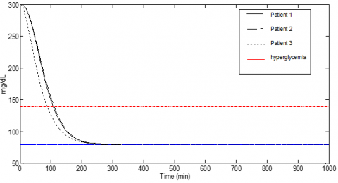
Figure 1. Glucose concentration using adaptive synergetic control
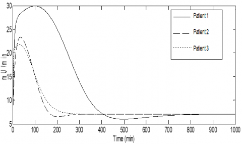
Figure 2. Insulin concentration measurement using adaptive synergic control
In addition, glucose concentration figures for the three patients with diabetes are shown in Figure 1. Additionally, insulin concentration required for each patient, is shown in Figure 2.
Accordingly, simulation results indicate that the glucose concentration rates of these patients are constant thanks to normoglycemia and in all the cases the glucose is completely stabilized at the basal level in a reasonable time interval.
Furthermore, no hypoglycemia is detected; as a result, constancy is assured by controller despite parameter uncertainties’ results of these three patients with diabetes.
5.2 Performance robustness system analysis under multiple disturbances
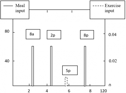
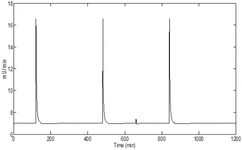
In the present silico experiment, robustness performance of the suggested controller was examined in view of multiple disturbances; such as meal ingestion events and exercise. Thus, all patients were introduced to three meals oral intake for 15 minutes at 8 am, 2 pm, and 8 pm (of 60 g of carbohydrate (CHO)). Additionally, a physical exercise disturbance at 5 pm for 20 minutes was also required (0.005 arbitrary units). These disturbances are measured by pulses’ frequencies as shown in Figure 3.
Figure 3. Meal and Exercise disturbances
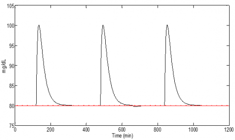
Figure 4. Blood glucose response of closed-loop system
Figure 5. Insulin infusion response of the closed-loop system
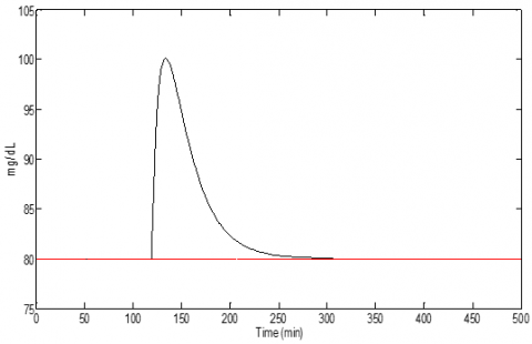
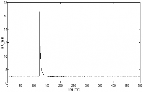
Thus, from the glucose-insulin profile in Figures 4, 5, it is revealed that when a patient is subjected to meal (CHO) every six waking hours, the BG level remains within tight regulation of 81±20 mg/dl by controlled infusion rate of insulin within limits of ±10mU/min over the basal dose. When the patient is subjected to specific exercise disturbance, the glucose level falls to 78 mg/dl, which is also within acceptable limit. The insulin dose is also well controlled between 0-36 mU/min so that the condition of hypo glycaemia never appears at the same time device delivery restriction is maintained, i.e. no clipping for negative infusion command is required.
It was concluded that “if a patient is subjected to meal, his blood glucose level does not exceed normalcy limit using ASC infusion rate of insulin.” Moreover, the findings suggest that “if a patient practices sport (exercises disturbance), glucose concentration is maintained at a normal level.” Furthermore, the results indicate no existence of hypoglycemia and hyperglycemia problems in blood glucose level; in addition to that, the insulin infusion and settling time rate are within an acceptable limit, which indicate that ASC performs adequately well under multiple disturbances.
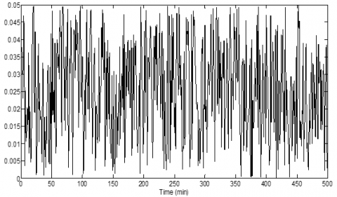
5.3 Analyzing the performance of the controller with actuator noise
In this experiment, the concept of new adaptive disturbance estimation technique has been used for the design of a synergetic controller can overcome the influence which unknown limit disturbance.
Figure 6 and Figure 7 show the glucose concentration level and the insulin concentration dose, and so the suggested controller tracked set point during meal and noise disturbances. Besides, the controller performance was assessed in terms of reducing the effect of the disturbance.
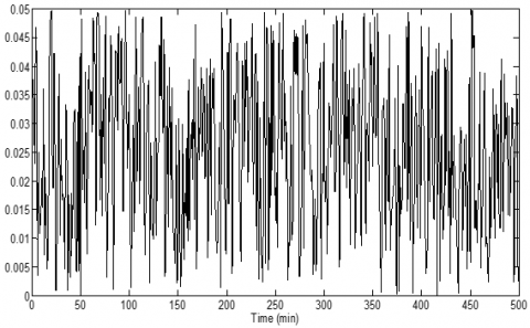
In Figure 8 the actuator noise is considered to be white color and assuming 0.05 a standard variation in the insulin pump as for the existing actual device [6].
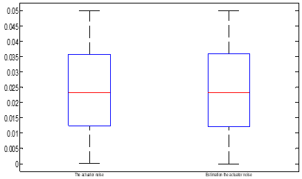
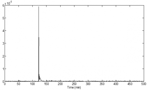
Figure 9 shows the estimation disturbance noise, in a finite time, the new adaptation is utilized to guarantee that the disturbance estimation will converge to the optimal approximate of disturbing noise. To check this, we compared the disturbance noise and the estimation disturbance noise, as shown in Figure 10 which is guaranteed the disturbance estimate converges to the optimal approximation.
It is also shown in Figure 11 that tracking estimation error according to the proposed method convergences faster than
according to the conventional adaptive control methods.
In this experiment, the patient model is subjected to controlled dietary meal of 60gm (equivalent carbohydrate taken orally (CHO)) for 15min each (duration of meal ingestion).
Figure 6. Glucose concentration with actuator noise
Figure 7. Insulin concentration with actuator noise
Figure 8. The actuator noise
Figure 9. Estimation the actuator noise
Figure 10. Box plot used to compare by the actuator noise and estimation the actuar noise
Figure 11. Estimation error eF
In The diabetes management as one of the challenging control problems in human regulatory systems has been discussed. The treatment of the disease via robust feedback control design has been considered.
In this study, a developed adaptive synergetic control for nonlinear control systems is designed using a new adaptive law. Besides, the synergetic control technique is applied for stabilizing a nonlinear model for type-I diabetic patient in presence of deterministic meal and activity disturbances and actuator noise for a robust closed-loop stability of the insulin delivery system. The asymptotic stability of the closed-loop system and convergence of the approximation are proven using Lyapunov stability method. The performance objective was to regulate the glucose level in face to disturbances represented by known meals and excise. The glucose-insulin response has shown very close regulation of blood glucose level with minimum overshoots and undershoots and acceptable limits of insulin infusion rate.
This stabilization was achieved in light of internal and external factors such as exercise and meal intake with stochastic noise. This suggests that the entire system is valid and vigor. Simulation results revealed the effectiveness and robustness of this technique despite accidental disturbances. The results suggest that this type of control strategies can be implemented practically using an embedded system with the precise implantable pump and sensor for a robust blood glucose control in patient.
|
G(t) |
Plasma glucose concentration. |
|
X(t) |
The insulin reduction effect on glucose concentration. |
|
I(t) |
Insulin concentration level in plasma. |
|
Ib |
Basal blood insulin. |
|
Gb |
The basal glucose concentrations. |
|
γ |
The pancreatic β- cells’ rate that release insulin after glucose insertion. |
|
h |
The above glucose sill value in which the pancreatic β- cells release insulin. |
|
n |
Measure of insulin consumed in plasma. |
|
u(t) |
The insulin dose rate. |
|
D(t) |
Represents a disturbance indicator. |
|
e |
The system error. |
|
$\psi$ |
The macro-variable. |
|
$\hat{F}$ |
Estimation of disturbance. |
[1] Jorge, B., Sergio, V., Beatriz, R., Jo, L. (2018). Insulin estimation and prediction. IEEE Control Systems Magazine, 38(1): 47-66. https://doi.org/10.1109/MCS.2017.2766312
[2] Paiva, H.M., Keller, W.S., da Cunha, L.G.R. (2020). Blood-glucose regulation using fractional-order PID control. Journal of Control, Automation and Electrical Systems, 31(1): 1-9. https://doi.org/10.1007/s40313-019-00552-0
[3] Mahmud, F., Isse, N.H., Daud, N.A.M., Morsin, M. (2017). Evaluation of PD/PID controller for insulin control on blood glucose regulation in a Type-I diabetes. AIP Conference Proceedings, 1788(1): 030072. https://doi.org/10.1063/1.4968325
[4] Al Helal, Z., Rehbock, V., Loxton, R. (2015). Modelling and optimal control of blood glucose levels in the human body. Journal of Industrial and Management Optimization (JIMO), 11(4): 1149-1164. https://doi.org/10.3934/jimo.2015.11.1149
[5] Sherif, S., Kralev, J., Slavov, T., Kunchev, V. (2020). Design of the H∞ regulator for the control of glucose concentration in patients with first type diabetes. IOP Conference Series: Materials Science and Engineering, 878(1): 012003. https://doi.org/10.1088/1757-899X/878/1/012003
[6] Patra, A.K., Mishra, A.K., Rout, P.K. (2020). Backstepping model predictive controller for blood glucose regulation in type-I diabetes patient. IETE Journal of Research, 66(3): 326-340. https://doi.org/10.1080/03772063.2018.1493404
[7] Kolesnikov, A., Veselov, G. (2000). Modern applied control theory: Synergetic Approach in Control Theory, vol. 2. (in Russian) Moscow – Taganrog, TSURE Press.
[8] Hadda, B., Larbi, C., Abdessalam, M. (2018). A new technique of second order sliding mode control applied to induction motor. European Journal of Electrical Engineering, 20(4): 399-412. https://doi.org/10.3166/EJEE.20.399-412
[9] Belouahchi, F., Merabet, E. (2020). Design of a new direct torque control using synergetic theory for double star induction motor. Journal Européen des Systèmes Automatisés, 53(6): 903-914. https://doi.org/10.18280/jesa.530616
[10] Astrom, K.J., Wittenmark, B. (1994). Adaptive Control. 2nd Edition. Addison-Wesley Pub Co.
[11] Toffolo, G., Bergman, R.N., Finegood, D.T., Bowden, C.R., Cobelli, C. (1980). Quantitative estimation of beta cell sensitivity to glucose in the intact organism: a minimal model of insulin kinetics in the dog. Diabetes, 29(12): 979-990. https://doi.org/10.2337/diab.29.12.979
[12] Vakili, S., ToosianShandiz, H. (2019). Back-stepping sliding mode control design for glucose regulation in type 1 diabetic patients. International Journal of Nonlinear Analysis and Applications, 10(2): 167-176. https://doi.org/10.22075/ijnaa.2019.4183
[13] Markakis, M.G., Mitsis, G.D., Papavassilopoulos, G.P., Ioannou, P.A., Marmarelis, V.Z. (2011). A switching control strategy for the attenuation of blood glucose disturbances. Optimal Control Applications and Methods, 32(2): 185-195. https://doi.org/10.1002/oca.900
[14] Hernández, A.G.G., Fridman, L., Levant, A., Shtessel, Y., Leder, R., Monsalve, C.R., Andrade, S.I. (2013). High-order sliding-mode control for blood glucose: Practical relative degree approach. Control Engineering Practice, 21(5): 747-758. https://doi.org/10.1016/j.conengprac.2012.11.015
[15] Yu, S., Yu, X., Shirinzadeh, B., Man, Z. (2005). Continuous finite-time control for robotic manipulators with terminal sliding mode. Automatica, 41(11): 1957-1964. https://doi.org/10.1016/j.automatica.2005.07.001
[16] Hou, M., Duan, G., Guo, M. (2010). New versions of Barbalat’s lemma with applications. Journal of Control Theory and Applications, 8(4): 545-547. https://doi.org/10.1007/s11768-010-8178-z