Güzin Tirkeş* | Neşe Çelebi | Cenk Güray
© 2021 IIETA. This article is published by IIETA and is licensed under the CC BY 4.0 license (http://creativecommons.org/licenses/by/4.0/).
OPEN ACCESS
A great deal of research has been undertaken in recent years related to facility capacity expansion and production planning problems under deterministic and stochastic constraints in the literature. However, only a small portion of this work directly addresses the issues faced by the food and beverage industry, especially in small-sized enterprises. In this study, a Mixed-Integer Linear Programming model (MILP) is developed for production planning and scheduling decisions for a small-size company producing syrup and jam products. The main constraint is that the multiple syrup and jam production lines in the model share the same limited-capacity module designed for inventory planning. To this end, the present model offers an efficient solution for executing a multi-product, multi-period production line by finding the most satisfactory strategy to match the right product with the useable capacity leading to profit maximization. The present approach is capable of coping with varying demands by offering a detailed costing procedure and implementing an effective inventory model.
mathematical modeling, optimization in food and beverage production, production scheduling, production planning, MILP, multi-product, multi-period
The food industry is a special area of engineering which faces certain difficulties quite frequently. These difficulties include uncertainty in resource allocation and inventory cost, and unexpected variations in supply, demand, and operation timing. Increasing competitive pressure in the business environment has increased the importance of planning and optimization. Although the major companies understand the importance of production process optimization and apply integrated process solutions, small and medium-sized enterprises still have problems of inefficiency due to the lack of such optimization efforts.
Production planning is a branch of industrial engineering which combines various engineering techniques with mathematical optimization to advance resource utilization while satisfying client demands in a given period [1]. Every organization needs a production plan to maximize its productivity. However, effective planning is a complex process and to supply the required amount of material, human resources, and related equipment needs through arrangements. Production process optimization that is directly related to planning and scheduling can face some risks in the food industry due to the nature of the product. Some of the aspects to consider are; the risk of perishing, the additional cost associated with cold storage, and the choice of frozen food over fresh products.
The following studies can be considered as milestone works in the scheduling-planning area regarding the food industry. Huddlestone and Vuuren established one of the first conceptual mathematical models for drawing an optimal pulping schedule using Linear Programming (LP) [2]. Viswanathan and Goyal recommended that production planning optimization could be accomplished by modifying production rate and/or cycle time, simultaneously [3]. As for the latter case, once a given stage is completed, the upcoming one starts either instantly or after an interphase delay aiming to manufacture the correct batch size going along with an efficient ordering policy for products with shelf lives.
Doganis and Sarimveis proposed a scheduling optimization model for yogurt production on a single-line basis over a six-day horizon production period. They used the MILP model for a weekly schedule where the objective function was to minimize all major sources of variable costs associated with the production schedule, such as changeover cost, inventory cost, and labor cost. They worked on real demand data, in which the model takes into consideration binary variables to indicate whether a setup takes place for exchange between two products. The model produced a complete production schedule for future demands, including inventory information [4].
Ertugrul and Işık presented a single-line production planning model for a winery to select new products to be produced, and to determine the quantity of the products to maximize profit. They used the branch and bound method to solve the problem, and the optimization results were obtained from a Mixed Integer Programming (MIP) model based on production times and total capacity in seconds [5].
Parthanadee and Buddhakulsomsiri considered a production scheduling problem in a canned fruit factory, where there are multi-products and multi-lines. To minimize the flowtime and tardiness-based measures, they applied real-time scheduling using setup dependent rules and tested the dispatching rules using discrete-event simulation modeling based on data pertaining to eleven months of seasonal history. They achieved the best results for their case by using a modified due date rule [6].
Habibollah and Kianehkandi proposed a weekly production scheduling optimization model based on a MILP model in a single production line producing four different types of milk in three working shifts. They worked on the daily demand data to minimize changeover, inventory, and labor costs. Binary variables were used to indicate whether setup exchange takes place between two products and whether the respective product is to be produced on a particular day. The model prepared the complete production schedule for a selected future horizon, including the sequence of products that should be produced every day, the respective quantities, and the inventory levels at the end of each day [7].
Kopanos, Puigjaner, and Georgiadis proposed a model for production planning, production scheduling in a multi-product and multi-stage process for the ice cream sector. The objective function of the model aims to minimize the makespan without considering the profit [8]. In 2012, the same group considered the production scheduling problem in a real-world multi-stage, multi-product ice cream production facility. They first presented a MIP continuous-time model (MIP-R) relying on the integrated modeling of all production stages by the introduction of several sets of integer cuts regarding the allocation and sequencing decisions and, then, proposed a MIP-based decomposition method to cope with large-scale production scheduling problems. They used binary variables to ensure sequential production [9].
Guimaraes studied a real-world multi-line, multi-product production planning problem in a beverage enterprise producing beer, soft drinks, mineral, and sparkling water. They aimed to create the annual production budget while minimizing the total setup, inventory, transfers, and overtime costs. They first formulated the problem as a MILP model comprising a multi-plant environment, where each plant has its demand. The storage capacity and planning horizon factors were taken in monthly periods, while binary variables were used for the setup process of a new product. Then, a new heuristic was developed according to the test results, which improved the current company practice [10].
In their paper, Xie and Lie discuss a meat production company, for which an asynchronous exponential serial production line is constructed [11]. The main problem leading to a decrease in production efficiency was determined by using a non-linear model solved by executing the methods introduced by Li and Meerkov [12]. At the end of the execution, the model observed the manual-technical problems in the machine set by performing a bottleneck analysis, and it was able to identify the machines whose improvement would lead to the largest increase in the throughput. It was seen that system productivity was increased significantly by reducing the downtime of the bottleneck machines thanks to the model applied.
Catala et al. proposed a multi-period, multi-product strategic planning model to increase profit generated in a juice manufacturing enterprise throughout a season, by deciding which fruit (apple/pear) to be processed during each day of the planning horizon. MILP model is used for optimization. Yet, the proposed model lacks flexibility due to the changing demand conditions [13].
The model by Bilgen and Çelebi differs from the others in the sense that they perform production scheduling and distribution planning by considering the perishing characteristics of the dairy products in the same MILP model. Another difference is that they acquire the demand data based on a simulation model [14].
Sel and Bilgen presented a hybrid solution using MILP and simulation for a real-world multi-product, multi-line production, and distribution planning approach in a soft drink company. Their planning horizon consists of four weeks with daily periods. They used randomly generated demand data with the objective function to minimize cost. Fix&Relax and Fix&Optimize MIP heuristics are applied alongside time-based capacity constraints. Using the hybrid method, they reached acceptable results [15].
The paper by Toledo et al. applies a genetic algorithm embedded with mathematical programming techniques to solve a synchronized and integrated two-level lot sizing and scheduling problem motivated by a real-world case in the soft drink sector. To minimize the inventory shortage and set-up costs, a MILP model was developed. The main aim of the model is to take lot-sizing and scheduling decisions simultaneously for raw material preparation/storage in tanks and soft drink bottling in several production lines. The model successfully fulfills this aim by a solution approach combining the Genetic Algorithm (GA) with the traditional linear programming techniques. In the execution process, the GA model decides the sequencing decisions for the production lots, whereas the linear programming model solves this “simplified” situation where only lot-sizing decisions are to be made [16].
Bilgen and Doğan applied a detailed model for maximizing the profit in the dairy industry. The inclusion of the factor for intermediate production increases the efficiency of the model. This model utilizes a deterministic demand for production planning [17].
Chatavithee, Piewthongngam, Pathumnakul developed a model for minimizing the cost during production planning for the frozen food industry. The model is developed on a single machine production line and, thus, the problem has an NP-hard structure [18].
Touil, Echchatbi, and Charkaoui proposed a model for production planning and scheduling in a multi-product and multi-stage process for the milk industry. The objective function of the model aims to minimize the makespan. Their model does not consider the profit factor [19].
Georgiadis et al. presented a mixed batch and continuous food makespan minimization model for the multi-product canned fish industry. The objective of the study is the minimization of the total production makespan [20].
As far as literature goes, the above-mentioned studies and some others propose solutions for production planning, scheduling, and optimization problems in the F&B industry. But it can be observed that there are only a few studies in the literature presenting optimization approaches for supporting production planning and scheduling in the fresh fruit sector including syrup and jam production especially when the requirements of this sector about multi-product and multi-period planning is considered.
Against this backdrop, the present research aims to develop a production planning model to optimize the production line at a company that has been active since 1971 producing jam and syrup from fresh and frozen fruit. The model takes into account tactical decisions such as selecting the type of product to be produced to meet the demand. The model aims to provide profit maximization with a multi-product, multi-period approach. The model combines a very detailed cost analysis background with an inventory to suit various demand scenarios.
2.1 Company description and research design
2.1.1 Company overview
This study was motivated by the effort to address the production planning and scheduling requirements in the Tarihi Yudumla syrup and jam Production Company. The enterprise started operations in 1971 in İzmir, Turkey. Currently, it produces three types of jams and four types of syrup both for retail and wholesale.
All the products of the company are subject to internationally recognized quality standards, such as the British retail food certificate (BRC), the international organization for standardization (ISO) certificate, and hazard analysis critical control point certificate (HACCP).
2.1.2 Production system
The working hours at the company are between 08:00 and 18:00. The daily production time does not exceed 10 h, except for jam production which begins at 06:00. By safety standards, the production cycle cannot exceed 24 h. Besides, the total working days in one month is 20.
Three production lines are producing three different types of jams and four different types of syrup all of which follow different lines. As a result, they are grouped into three, namely the jam group, the berry syrup group, and the lemonade. All products have different costs and selling prices.
The number of employees varies seasonally, increasing in high season. Each employee is assigned to a single line of product, with a likelihood of assignment to other lines should there be any mechanical disruptions.
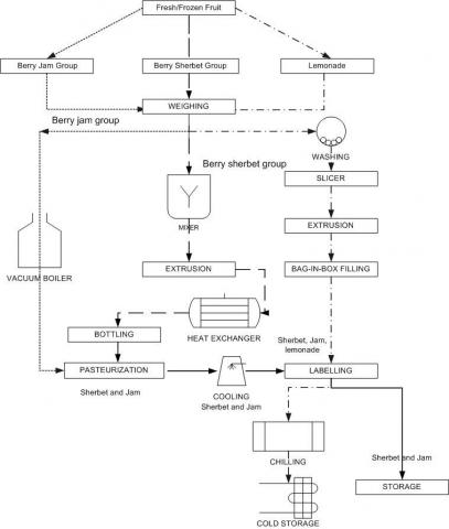
According to the total production amounts and sales of the company: for the jam group (blueberry jam, raspberry jam, black mulberry jam) 67%; for the berry syrup group (black mulberry syrup, blueberry syrup, red currant syrup) 62.7%; and for the lemonade group, 74.6% of the total sales are made to the most major client referred to as “Company X” in the rest of the study. This significant percentage, demand by Company X, is the driving factor in the production planning process. Tarihi Yudumla, the company under study sells its products to not just Company X, but also others (referred to as Company Y) at different prices. The demand has to be supplied on schedule and tardiness is not allowed; however, there is no penalty cost. The lemonade syrup can be supplied earlier due to the cold storage facilities available, which necessitates an inventory cost charge. In Figure 1, the process flow of all products is represented schematically.
Figure 1. Process flow
Accordingly, fresh and/or frozen fruit comes from the suppliers. All product ingredients require a weighing process. To produce jam, upon weighing sugar and fruit they are transferred into a vacuum boiling facility, where the mixture is boiled for 150 min at 560℃ and, then, bottled. The next stage is pasteurization, which is conducted for 15 min at 90℃. The product is, then, cooled for another 15 min and forwarded to the labelling stage and subsequent storage. The straight arrows (à) represent that pasteurization, cooling, and labelling machines are used both for syrup and jam production. The berry syrup batch production follows a different line; after weighing and blending, the mixture needs to be squeezed and filtered in the extrusion. Then, the mixture is transferred into the heat exchanger for heating up to 150 min at 90℃. After heating; bottling, pasteurization, cooling, and labelling processes are conducted. The third production line starts with an initial washing process, followed by slicing and mixing with sugar. After that, the extrusion process is conducted to obtain the fruit extract, which is subsequently diluted with water, and the end product is bottled in bag boxes and labelled. Among the products, only lemonade is chilled and stored in cold storage.
2.1.3 Machine capacities
Every machine has its production capacity. The same weighing and labelling machines are used for all product groups in all lines, whereas the pasteurization and cooling machines are used only for the syrup and jam lines. The transition between products is sequence-dependent. The machines are cleaned before any new batch arrives for processing; besides, there is a setup time between each processing regardless of whether the same or a different product arriving in. In Table 1, the machine capacities appear in kilograms, along with production times for each group.
Table 1. Machine capacities and related process times
|
Lemonade |
Kg |
Min |
|
Weighing |
40 |
0.50 |
|
Washing |
20 |
15.00 |
|
Slicing |
5 |
1.00 |
|
Extrusion |
20 |
2.55 |
|
Bag-in-box filling |
5 |
0.50 |
|
Labeling |
1000 |
40.00 |
|
Chiller |
3000 |
1440.00 |
|
Jam Group |
Kg |
Min |
|
Weighing |
40 |
0.50 |
|
Vacuum Boiling |
100 |
150.00 |
|
Pasteurization |
70 |
15.00 |
|
Cooling |
70 |
15.00 |
|
Labeling |
300 |
60.00 |
|
Syrup Group |
Kg |
Min |
|
Weighing |
40 |
0.50 |
|
Mixer |
7 |
3.00 |
|
Extrusion |
23.50 |
3.00 |
|
Heat Exchanger |
220 |
150.00 |
|
Bottling |
220 |
35.00 |
|
Pasteurization |
70 |
15.00 |
|
Cooling |
70 |
15.00 |
|
Labeling |
70 |
14.00 |
This research aims to develop a production planning optimization model to improve the production of a real-world multi-stage and multi-line syrup and jam production company producing multiple products for both retail and wholesale with a limited capacity and whether the demand is either certain or uncertain for which forecasting is required. The model working on the predicted demand data considers tactical decisions, such as selecting the kind of product to be produced so that the demand can be satisfied [21]. To cope with such barriers, a specific mathematical model designed for production planning will be used and demonstrated based on the case company.
2.1.4 Data collection
This section describes the data collection procedure in the Tarihi Yudumla Company. This information was primarily gathered through in-depth interviews with the company’s managers and workers, as well as through the stopwatch method, and remote monitoring using Intelligent Video Management System (IVMS), and client mail orders.
Selecting the interviewees was a basic step in this research process in light of the fact that their insight, experience, aptitudes, and readiness to collaborate could affect the amount of information available. Unstructured interviews were chosen, based on which the interviewees were asked to provide answers to open-ended questions and further elaborate on any specific issue for the qualitative research objectives [22, 23]. The main purpose of the interviews was to understand the production process and identify the main problems of the company during production scheduling. The decimal minute stopwatch method is used in the production process timings and the calculation of work cycles. Therefore, the duration of all the activities is inserted in the model in terms of minutes. The interviews were held in two months, with about an hour allocated to each respondent.
The data collected included the clients’ mail orders specifying their demands for products. Taking into account this initial step, a list of required documentation including financial and statistical information was created comprising:
In the third step of data collection, the information collected based on the stopwatch method and remote monitoring offered further insight into the processes of production. Each process is recorded and, using the IVMS system, the actual production process is followed and analyzed. The workloads and production process times are calculated for each product group according to the record.
2.2 Model formulation of a deterministic MILP for multi-product, multi-period production planning
This study designs a deterministic production planning model including probabilistic production capacities and inventory [24]. The problem that is examined in this section of the study has the following features:
The objective of the production-planning model in this study is to decide which product to produce and in what amount, having the ultimate goal as maximizing the profit. The model formulation presented in this study includes both integer and binary variables, with the latter applied to represent the production hierarchy in overlapping processes. The basic characteristics of the proposed model are as follows:
(i) The predicted demand amounts obtained using various forecasting methods such as the time series model considering seasonality and fuzzy applications were used in this model as well as the deterministic demand [21]. The amount of products to be made are planned on a monthly basis with a preference for early release prior to due date.
(ii) The inventory of the products is assumed to be 0 for the initial point. The jam and syrup product groups are stored in an ordinary non-air-conditioned depot. However, lemonade has to be chilled and, then, stored in cold-storage, and inventory cost is charged accordingly.
(iii) The production cost components of each product including, raw material, utilities, labor, and other parameters are collected from the company’s records. Using all the cost components for fruit, sugar, etc., the cost for the production of a unit of each product can be calculated. After that, in the objective function, the difference between the unit selling price and the unit cost is given as the profit coefficient. In cost calculation, the study only considers the company’s normalized values and no others for data protection.
(iv) The number of cycles required for producing a monthly demand is calculated by dividing the required amount of raw material by the capacity of the related machine. The cycle time of each machine is calculated by adding the setup time to the operating time for producing the full capacity amount. By multiplying the cycle time with the number of cycles required for producing the demand, the total time required for production can be achieved.
The probabilistic yearly production capacities are included as the upper limits of production to limit excess production, which can put an extra burden on the inventory that cannot be turned into sales. MCS (Monte Carlo Simulation) is used for simulating this scenario by random number generation and defining the probabilistic limit points [24].
2.2.1 Products
As stated earlier, the selling prices and profits made from each product differ when it comes to Company X (the major client) and Company Y (minor clients). In the result section, their effects will be different for the objective function which calls for the products to be divided into two groups as X and Y. The end product types are indexed in the model as follows:
This general model has additional room for new products to be made within the already available lines.
2.2.2 Production times
The machine capacities, where there is a shift in the type of products to be made, are sequence-dependent. Once all demanded products are produced, should there be any surplus capacity, the model assigns this capacity to produce the most profitable item. Additionally, there are setup times in between each process which has to be deduced from the determined production period in minutes. The constraint limitations are also calculated according to monthly working times in minutes for each machine from which value the setup times are eventually deduced as well.
2.2.3 Indices
The following indices are defined for the model:
i=number of products; {i=1,2,3,…,n}
i=1,…,k (jam)
i=k+1,…,(n-1) (syrup)
i=n (lemonade)
t=number of periods in the planning horizon (months); {t=1,2,3,…,12}
2.2.4 Parameters
The following parameters are defined for the model:
Wi = Weighing time for ith product; (min) {i=1,..,n}
WFi = Washing time for ith product; (min) {i=n}
Si = Slicing time for ith product; (min) {i=n}
ESi = Extrusion time for ith product; (min) {i=k+1,…,n}
BSi = Bottling time for ith product; (min) {i=1,…,n}
LJi = Labelling time for ith product; (min) {i=1,…,n}
BOi = Vacuum Boiling time for ith product; (min) {i=1,…,k}
PJi = Pasteurization time for ith product; (min) {i=1,…,(n-1)}
CJi = Cooling time for ith product; (min) {i=1,…,(n-1)}
Mi = Mixing time for ith product; (min) {i=k+1,…,(n-1)}
HEi = Heat exchanger time for ith product; (min) {i=k+1,…,(n-1)}
TICi = Total inventory capacity for ith product; (kg) {i=1,…,n}
DTit = Total demand for ith product for Company X and other companies in tth month; (kg) {i=1,…,7; t=1,.,12}
PXi = Profit we get from selling to Company X for one unit of ith product; (₺) {i=1,...,n}
PYi = Profit of other companies for one unit of ith product; (₺) {i=1,...,n}
PCit = Probabilistic capacities for ith product in tth month (kg) {i=1,…,7; t=1,.,12}
ici = Inventory holding cost for ith product; (₺) {i=1,...,n}
cwi = Amount of fruit to be weighed for producing one unit of ith product (kg); {i=1,…,n}
wfi = Amount of fruit to be washed for producing one unit of ith product (kg); {i=n}
si = Amount of fruit to be sliced for producing one unit of ith product (kg); {i=n}
esi = Amount of fruit to be extruded for producing one unit of ith product (kg); {i=k+1,…,(n)}
bi = Amount of fruit to be boiled for 1 unit of ith product (kg); {i=1,…,k}
mi = Amount of fruit to be mixed for 1 unit of ith product (kg); {i=k+1,…,(n-1)}
wci = Maximum cyclic capacity of the weighing machine for ith product (kg/cycle); i=1,…,n}
wfci = Maximum cyclic capacity of the washing machine for ith product (kg/cycle); {i=n}
sfci = Maximum capacity of the slicing machine for ith product (kg/cycle); {i=n}
esci = Maximum capacity of the extrusion machine for ith product (kg/cycle); {i=k+1,…,(n)}
bsci = Maximum capacity of the bottling machine for ith product (kg/cycle); {i=1,…,n}
ljci = Maximum capacity of the labeling machine for ith product (kg/cycle); {i=1,…,n}
bjci = Maximum capacity of the boiling machine for jam for ith product (kg/cycle); {i=1,…,k}
pjci = Maximum capacity of the pasteurization machine for ith product (kg/cycle); {i=1,…,(n-1)}
cjci = Maximum capacity of the cooling machine for products for ith product (kg/cycle); {i=1,…,(n-1)}
mci = Maximum capacity of the mixing machine for syrup for ith product (kg/cycle); {i=(k+1),…,(n-1)}
heci = Maximum capacity of the heat exchanger machine for ith product (kg/cycle); {i=1,...,(n-1)}
wei = Weighing time for one unit of ith product (min); {i=1,…,n}
wfti = Washing time for one unit of ith product (min); {i=n}
sfti = Slicing time for one unit of ith product (min); {i=n}
esti = Extrusion time for one unit of ith product (min); {i=k+1,…,(n)}
bsti = Bottling time for one unit of ith product (min); {i=1,...,n}
ljti = Labeling time for one unit of ith product (min); {i=1,…,n}
bjti = Boiling time for one unit of ith product (min); {i=1,…,k}
pjti = Pasteurization time for one unit of ith product (min); {i=1,...,(n-1)}
cjti = Cooling time for one unit of ith product (min); {i=1,…,(n-1)}
mti = Mixing time for one unit of ith product (min); {i=(k+1),...,(n-1)}
heti = The heat exchanger machine process time for one unit of ith product (min); {i=1,...,(n-1)}
ici = Inventory cost of one unit of ith product (₺);
M= Large integer number
2.2.5 Decision variables
The following decision variables are defined for the model:
Xit = Amount of ith product produced for Company X in tth month; {i=1,...,n; t=1,.,12}
Yit = Amount of ith product produced for other companies in tth month; {i=1,...,n; t=1,...,12}
ITit = Inventory amount of ith product in tth month; (kg) {i=1,…,n; t=1,…,12}
bqit = Binary variable for ith product pasteurized in tth month; {i=1,...,n; t=1,.,12}
bkit = Binary variable for ith product cooled in tth month; {i=1,...,n; t=1,.,12}
2.2.6 Objective function–profit maximization
The objective function includes the subtraction of the production cost which is calculated for one unit of product, from the selling price for raw materials, labor, inventory holding, and utility including water and electrical consumption. The raw material costs remain the same for an entire year as purchased in wholesale by the company at a fixed price.
$\operatorname{Max} \mathrm{Z}=\sum_{i=1}^{n} \sum_{t=1}^{12} P X_{i} X_{i t}+\sum_{i=1}^{n} \sum_{t=1}^{12} P Y_{i} Y_{i t}$-$\sum_{i=1}^{n} \sum_{t=1}^{12} i c_{i} I T_{i t}$ (1)
The objective function Eqn. (1) represents the profit made for each product. Which equals PXiXit for those sold to Company X in a given month t, and equals PYiYit for those sold to Company Y. The net profit Z is calculated by subtracting the inventory cost from the total profit.
2.2.7 Constraints
The model constraints are determined using cycle times, which are calculated using capacity limits.
The first constraint in Eq. (2) is the one for weighing sugar and fruit for production. cwiXit demonstrates fruit and sugar amount should be weighed for 1 unit of the ith product; wci indicates maximum machine capacity for one cycle for the ith product, and wti indicates the total weighing time including setup times for one cycle for the ith product. This constraint indicates that the entire total sugar and fruit weighing process for one unit product cannot exceed the total working time of the weighing machine in a given month.
$\sum_{i=1}^{n}\left[\sum_{t=1}^{12}\left(c w_{i} X_{i t} / w c_{i}\right) w e_{i}\right.$$\left.+\sum_{t=1}^{12}\left(c w_{i} Y_{i t} / w c_{i}\right) w e_{i} \leq W_{i}\right]$ (2)
Time limitation is calculated in every constraint as follows; the daily working hours are 10 h which is equal to 600 min for all machines, except the vacuum boiling and the heat exchanger. Only these two machines work 12 h a day, which is equal to 720 min.
For the weighing machine, the total working time in a day is 600 min. When the monthly working time is considered, it will be 600*20= 12000 min. The machines do not operate the entire day due to the waiting times of the processes and also preliminary times. The total setup times are subtracted from monthly working times. The setup time for the weighing machine includes carrying the fruit boxes to weighing, storage, and production. The weighing machine is the first stage in the process line, which means there is no for any previous job. Other machines have process waiting times.
Constraints 3 and 4 that appear in the following are related to lemonade production. The constraints represent washing and slicing processes, respectively.
$\sum_{i=n}^{n}\left[\sum_{t=1}^{12}\left(w f_{i} X_{i t} / w f c_{i}\right) w f t_{i}\right.$$\left.+\sum_{t=1}^{12}\left(w f_{i} Y_{i t} / w f c_{i}\right) w f t_{i} \leq W F_{i}\right]$ (3)
$\sum_{i=n}^{n}\left[\sum_{t=1}^{12}\left(s_{i} X_{i t} / s f c_{i}\right) s f t_{i}\right.$$\left.+\sum_{t=1}^{12}\left(s_{i} Y_{i t} / s f c_{i}\right) s f t_{i} \leq S_{i}\right]$ (4)
The constraint 5 is for the extrusion machine, which is used both for syrup and lemonade products.
$\sum_{i=k+1}^{(n)}\left[\sum_{t=1}^{12}\left(e s_{i} X_{i t} / e s c_{i}\right) e s t_{i}\right.$$+\sum_{t=1}^{12}\left(e s_{i} Y_{i t} / e s c_{i}\right)$ est $\left._{i} \leq E S_{i}\right]$ (5)
Constraints 6 and 7 are related to the bottling and labelling processes for all products.
$\sum_{i=1}^{n}\left[\sum_{t=1}^{12}\left(X_{i t} / b s c_{i}\right) b s t_{i}+\sum_{t=1}^{12}\left(Y_{i t} / b s c_{i}\right) b s t_{i} \leq B S_{i}\right]$ (6)
$\sum_{i=1}^{n}\left[\sum_{t=1}^{12}\left(X_{i t} / l j c_{i}\right) l j t_{i}+\sum_{t=1}^{12}\left(Y_{i t} / l j c_{i}\right) l j t_{i} \leq L J_{i}\right]$ (7)
The constraint 8 is used only for jam production.
$\sum_{i=1}^{k}\left[\sum_{t=1}^{12}\left(b_{i} X_{i t} / b j c_{i}\right) b j t_{i}+\sum_{t=1}^{12}\left(b_{i} Y_{i t} / b j c_{i}\right) b j t_{i} \leq B O_{i}\right]$ (8)
Constraints 9 and 15 are related to the pasteurization and cooling processes for both jam and syrup, and constraints 10 to 14 are binary variables in pasteurization and cooling processes, giving a profit-based hierarchy for the production processes.
$\sum_{i=1}^{(n-1)}\left[\sum_{t=1}^{12}\left(X_{i t} / p j c_{i}\right) p j t_{i}+\sum_{t=1}^{12}\left(Y_{i t} / p j c_{i}\right) p j t_{i} \leq P J_{i}\right]$ (9)
$\sum_{i=1}^{(n-1)}\left[\sum_{t=1}^{12} X_{i t}-\sum_{t=1}^{12} M * b q_{i t} \leq 0\right]$ (10)
$\sum_{i=1}^{(n-1)}\left[\sum_{t=1}^{12} Y_{i t}-\sum_{t=1}^{12} M * b q_{i t} \leq 0\right]$ (11)
$\sum_{i=1}^{(n-1)}\left[\sum_{t=1}^{12} b q_{i t}-\sum_{t=1}^{12} b k_{i t}=0\right]$ (12)
$\sum_{i=1}^{(n-1)}\left[\sum_{t=1}^{12} X_{i t}-\sum_{t=1}^{12} M * b k_{i t} \leq 0\right]$ (13)
$\sum_{i=1}^{(n-1)}\left[\sum_{t=1}^{12} Y_{i t}-\sum_{t=1}^{12} M * b k_{i t} \leq 0\right]$ (14)
$\sum_{i=1}^{(n-1)}\left[\sum_{t=1}^{12}\left(X_{i t} / c j c_{i}\right) / c j t_{i}+\sum_{t=1}^{12}\left(Y_{i t} / c j c_{i}\right) c j t_{i} \leq C J_{i}\right]$ (15)
Constraints 16 and 17 are related to syrup production, including mixer and heat exchanger processes.
$\sum_{i=k+1}^{(n-1)}\left[\sum_{t=1}^{12}\left(m_{i} X_{i t} / m c_{i}\right) / m t_{i}\right.$$\left.+\sum_{t=1}^{12}\left(m_{i} Y_{i t} / m c_{i}\right) m t_{i} \leq M_{i}\right]$ (16)
$\sum_{i=k+1}^{(n-1)}\left[\sum_{t=1}^{12}\left(X_{i t} / h e c_{i}\right) / h e t_{i}\right.$$\left.+\sum_{t=1}^{12}\left(Y_{i t} / h e c_{i}\right) h e t_{i} \leq H E_{i}\right]$ (17)
The constraint 18 represents the inventory capacity for all products. The initial inventory of all products is assumed to be 0, as, given in Eq. (19).
$\sum_{i=1}^{n} \sum_{t=1}^{12}$$I T_{i t} \leq T I C_{i}$ (18)
$\sum_{i e 1}^{n} I T_{i t}=0$ at $\mathrm{t}=0$ (19)
Constraints 20, 21, and 22 represent the inventory level of product groups. According to the given limitations, after satisfying the client demands, the model produces profitable products in the remaining capacities and times. The constraint 22 limits the production level. The total amount of the product in the inventory cannot exceed the total demand.
$\sum_{t=1}^{12} \sum_{i=1}^{n}\left(X_{i t}+Y_{i t}\right)-D T_{i t}+I T_{(t-1)} \geq 0$ (20)
$\sum_{t=1}^{12} \sum_{i=1}^{n}\left(I T_{i t}-I T_{i(t-1)}-\left(X_{i t}+Y_{i t}\right)+D T_{i t}\right) \geq 0$ (21)
$\sum_{t=1}^{12} \sum_{i=1}^{n}\left(X_{i t}+Y_{i t}\right)+I T_{(t-1)} \leq P C_{i t}$ (22)
The constraint 23 represents the total demand values for X and Y and, finally, 24 and 25 represent the production for X and Y. The total amount of these two has to be greater than 0.
DTit>=0 (23)
Xit>= 0 (24)
Yit>= 0 (25)
The maximum production amount should not be less than the monthly demand while the total production should not exceed the annual demand for any of the items, the reason being that no unsold product is to be kept in the inventory. To make this scenario possible MCS is applied and in constraint 22 the related results are used as production limits.
The proposed MILP model is executed first for 12 months based on demands anticipated in our previous study [21] to test its effectiveness and after that, for the following two years, the MILP model is executed with actual demands.
As stated before, the initial inventory for all products is assumed to be 0, which implies that all products are sold. Table 2 presents the total annual amount of production, the total demand for Company X, the total amount of products sold to other companies (Y), and, the profit for the first 12 months. Table 3 represents the deterministic MILP model results for the same period. For data protection, proportionally modified data is used here.
The deterministic MILP model results presented in Table 3 show a more profitable production scenario. In the proposed model, the company produces 15% more products and makes 25% more profit using the MILP model, assuming that all the products including the inventory are sold.
Table 4 represents actual profit versus profit acquired from the deterministic model for years 2017 and 2018.
Table 2. Actual production of the company
|
Product Type |
Amount of Production (kg/year) |
Company X demand (kg/year) |
Amount sold to other companies (kg/year) |
Profit (1000₺/year) |
|
Black mulberry jam |
7684 |
3234 |
4446 |
11970 |
|
Raspberry jam |
4955 |
3779 |
1176 |
22245 |
|
Blueberry jam |
1437 |
776 |
661 |
3800 |
|
Black mulberry syrup |
62959 |
21916 |
41991 |
190900 |
|
Blueberry syrup |
16512 |
15708 |
2641 |
46990 |
|
Currant syrup |
12648 |
8736 |
4440 |
35390 |
|
Lemonade |
115000 |
96500 |
18500 |
317980 |
Table 3. Production with MILP deterministic model
|
Product Type |
Amount of Production (kg/year) |
Company X demand (kg/year) |
Amount sold to other companies (kg/year) |
Profit (1000₺/year) |
|
Black mulberry jam |
5216 |
3234 |
1982 |
9160 |
|
Raspberry jam |
4782 |
3779 |
1003 |
21500 |
|
Blueberry jam |
1236 |
776 |
460 |
3050 |
|
Black mulberry syrup |
56928 |
21916 |
35012 |
169295 |
|
Blueberry syrup |
30673 |
15708 |
14965 |
101490 |
|
Currant syrup |
18773 |
8736 |
10037 |
56180 |
|
Lemonade |
136390 |
96500 |
39890 |
423980 |
Table 4. Actual profit versus profit acquired from the deterministic model for years 2017 and 2018
|
|
Profit (1000₺ /year) |
|||
|
Product Type |
Actual |
Deterministic Model |
||
|
2017 |
2018 |
2017 |
2018 |
|
|
Black mulberry jam |
9185 |
17355 |
30800 |
31135 |
|
Raspberry jam |
54294 |
81832 |
67924 |
68404 |
|
Blueberry jam |
6547 |
10980 |
21649 |
25094 |
|
Black mulberry syrup |
119844 |
175628 |
162358 |
167206 |
|
Blueberry syrup |
28022 |
74467 |
124457 |
129806 |
|
Currant syrup |
24447 |
61051 |
118293 |
125558 |
|
Lemonade |
456199 |
377053 |
561706 |
558612 |
|
Total |
698539 |
798365 |
1087200 |
1105830 |
When the model is re-executed with the demand values of 2017 and 2018, it can easily be observed that the MILP model developed to propose a much more profitable production planning scenario that can increase the profitability of the company 55% in 2017 and 39% in 2018. Keeping in mind the basic assumptions of the model, these proportions can be realized by the company with an effective advertisement and customer relations policy. These results show the efficiency of the model in terms of both production and inventory planning. This comparative study shows that the MILP model offers better results than the current production pattern at the company.
The MILP model can be successfully adapted to food and beverage production by developing a more effective schedule and prioritizing certain machines and products as required. The model leads the way to flexible production systems, especially for small-sized companies which need to adapt to unanticipated demand variations. Besides, the approach allows users to effectively determine their production alternatives and capacity utilization, with the ultimate goal to improve the decision support system.
The MILP model presented here can be regarded as a successful example in the industry based on inventory. The model leads the way to strategic decisions for maximizing the profit by satisfying the demands by the virtue of using binary variables to demonstrate an effective production schedule and by matching the right product with the right machine. In this way, the most efficient combination of products can be made within the given capacity conditions based on profit maximization and detailed costing procedure.
In detail, the model is able to analyse whether a requested demand can be satisfied, and in which direction the remaining capacity after the demand satisfaction should be used to reach a profitable production scheduling. In addition to this, an inventory-planning model is developed to check the level of inventory on a monthly basis for each product based on this scheduling scenario.
As a result, this model can be regarded as a unique approach for optimizing the production planning and scheduling process for F&B production companies, whereas it can also function as a decision-support tool.
As for future work, certain improvements can obviously take place. To begin with, the proposed model currently involves three production lines whose number can be increased depending on the number of products planned to be produced based on demand. Next, the machines used here are the conventional equipment used in the jam and syrup industry; however, it is possible to modify the model by changing capacities for different machines on the same line.
[1] Riggs, J. (1981). Production Systems: Planning Analysis and Control. New York: Wiley.
[2] Van Vuuren, J.H., Huddlestone, G.E. (1999). Seeking optimality in fruit pulping schedules: A case study. ORiON, 15: 25-51.
[3] Viswanathan, S., Goyal, S.K. (2002). On'Manufacturing batch size and ordering policy for products with shelf lives'. International Journal of Production Research, 40(8): 1965-1970. https://doi.org/10.1080/00207540210123661
[4] Doganis, P., Sarimveis, H. (2007). Optimal scheduling in a yogurt production line based on mixed-integer linear programming. Journal of Food Engineering, 80(2): 445-453. https://doi.org/10.1016/j.jfoodeng.2006.04.06
[5] Ertuğrul, İ., Işik, T. (2009). Production planning for a winery with mixed integer programming model. Ege Academic Review, 9(2).
[6] Parthanadee, P., Buddhakulsomsiri, J. (2010). Simulation modeling and analysis for production scheduling using real-time dispatching rules: A case study in canned fruit industry. Computers and Electronics in Agriculture, 70(1): 245-255. https://doi.org/10.1016/j.compag.2009.11.002
[7] Doganis, P., Sarimveis, H. (2007). Optimal scheduling in a yogurt production line based on mixed integer linear programming. Journal of Food Engineering, 80(2): 445-453. https://doi.org/10.1016/j.jfoodeng.2006.04.062
[8] Kopanos, G.M., Puigjaner, L., Georgiadis, M.C. (2011). Production scheduling in multiproduct multistage semicontinuous food processes. Industrial Engineering & Chemistry Research, 50(10): 6316-6324. https://doi.org/10.1021/ie2001617
[9] Kopanos, G.M., Puigjaner, L., Georgiadis, M.C. (2012). Efficient mathematical frameworks for detailed production scheduling in food processing industries. Computers and Chemical Engineering, 42: 206-216. https://doi.org/10.1016/j.compchemeng. 2011.12.015
[10] dos Santos Guimaraes, L.F.R. (2013). Advanced production planning optimization in the beverage industry. Engineering.
[11] Xie, X., Li, J. (2012). Modeling, analysis and continuous improvement of food production systems: A case study at a meat shaving and packaging line. Journal of Food Engineering, 113(2): 344-350. https://doi.org/10.1016/j.jfoodeng.2012.05
[12] Li, J., Meerkov, S.M. (2009). Production Systems Engineering. Springer Science & Business Media.
[13] Catalá, L.P., Moreno, M.S., Durand, G.A., Blanco, A.M., Bandoni, A. (2015). Optimal production planning of concentrated apple and pear juice plants. Iberoamerican Journal of Industrial Engineering, 5(10): 172-187. https://doi.org/10.13084/2175-8018.v05n10a13
[14] Bilgen, B., Celebi, Y. (2013). Integrated production scheduling and distribution planning in dairy supply chain by hybrid modelling. Annals of Operational Research, 211: 55-82. https://doi.org/10.1007/s10479-013-1415-3
[15] Sel, Ç., Bilgen, B. (2014). Hybrid simulation and MIP based heuristic algorithm for the production and distribution planning in the soft drink industry. Journal of Manufacturing Systems, 33(3): 385-399. https://doi.org/10.1016/j.jmsy.2014.01.002
[16] Toledo, C.F.M., de Oliveira, L., de Freitas Pereira, R., Franca, P.M., Morabito, R. (2014). A genetic algorithm/mathematical programming approach to solve a two-level soft drink production problem. Computers & Operations Research, 48: 40-52. https://doi.org/10.1016/j.cor.2014.02.012
[17] Bilgen, B., Dogan, K. (2015). Multistage production planning in the dairy industry: A mixed-integer programming approach. Industrial and Engineering Chemistry Research, 54(46): 11709-11719. https://doi.org/10.1021/acs.iecr.5b02247
[18] Chatavithee, P., Piewthongngam, K., Pathumnakul, S. (2015). Scheduling a single machine with concurrent jobs for the frozen food industry. Computers and Industrial Engineering, 90: 158-166. https://doi.org/10.1016/j.cie.2015.09.004
[19] Touil, A., Echchatbi, A., Charkaoui, A. (2016). A MILP model for scheduling multistage, multi products milk processing. IFAC-PapersOnline, 49(12): 869-874. https://doi.org/10.1016/j.ifacol.2016.07.884
[20] Georgiadis, G.P., Ziogou, C., Kopanos, G.M., Garcia, M., Cabo, D., Lopez, M., Georgiadis, M.C. (2018). Production scheduling of multi-stage, multi-product food process industries. In Proceedings of the 28th European Symposium on Computer-Aided Process Engineering, 43: 1075-1080. https://doi.org/10.1016/B978-0-444-64235-6.50188-1
[21] Tirkeş, G., Güray, C., Çelebi, N. (2017). Demand forecasting: A comparison between the holt-winters, trend analysis, and decomposition models. Tehnicki Vjesnik. https://doi.org/10.17559/TV-20160615204011
[22] Taylor, S.J., Bogdan, R. (1998). Introduction to Qualitative Research Methods: A Guide Book and Resource (3rd ed.). Hoboken, NJ, US: John Wiley & Sons Inc.
[23] Robson, C. (2002). Real-World Research: A Resource for Social Scientists and Practitioner-Researchers (2nd ed.). Oxford: Blackwell Publishers Ltd.
[24] Tirkeş, G. (2016). Multi-Product, Multi-Stage Production Planning Model and Decision Support System Suggestion for F&B Industry. PhD diss., Atılım University.