Samsani Saritha | Elliriki Mamatha* | Chandra S. Reddy | Krishna Anand
© 2020 IIETA. This article is published by IIETA and is licensed under the CC BY 4.0 license (http://creativecommons.org/licenses/by/4.0/).
OPEN ACCESS
Computing and logistics management systems have a wide area of applications with compound Poisson process Markov system with a batch servicing facility where customers arrive either independently or batches for service into the multi-server queues. The service of the customers is processed either independently or batch-wise based on the requirement of various sizes. The order of service has been found to follow First Come First Service while customers arrive according to the exponential distribution. A mathematical model is proposed to process customers by using generalized spectral expansion method. The explicit type required to service the system is measured as buffer size. For accurate assessment of performance, numerical results have been depicted in graphical form.
mean queue length, batch arrivals and batch services, QBD – M, multi-server system, compound poisson process
In the present era of multi-server computers, the service capacity of the communication and its performance can be a major bottleneck in high-performance systems. As a result, its values are critical for the success of any application. A general communication system consists of the network interconnection [1-3] with notes where the packets are serviced. In order to perform parallel computations, the processors have to compute the packets along several communication lines [4]. Apart from the accuracy of computation, the role of communication also plays a significant impact in research areas of batch size service parallel computing systems.
Achieving a significant level of performance has its challenges in modeling and design of a fault-tolerant system [5]. However, the fact is that the customers' expectation concerning the availability and this performance remains the same despite a vast increase in communication and computational services. There are plenty of problems in management [6, 7], computer and communications which need to model with a multi-server system of service of a single queue [8]. The instantaneous arrival and service rate may depend largely on the state of the environment while it may also depend on the number of customers present to a smaller extent.
Batch Markovian Arrival Process (BMAP) in the discrete queuing system gained importance since it has ample applications in numerous fields and is used to predict performance measures such as congestion, management control models, web streaming and related fields [9-13]. BMAP is successfully applied for modeling aggregated Internet Protocol (IP) traffic [14]. Chakka and his team [15] contributed their work for the compound Poisson process (CPP) with a finite buffer of various parameters. Traffic with bursty nature in the fields of complex multimedia traffic applications such as voice over internet protocol (VOIP), teleconferences, web streaming have been modeled in their analysis.
The literature of the batch process and servicing for Markov modulated Poisson process (MMCP) is proposed in the works author Lee [16], Goswami [17], Niu [18] studied streaming process analysis for video services by modeling with bursty nature. Choudhury [19] gave evidence that BMAP is a good approach to service the packets in internet traffics. Dimitriou [20] proposed a righteous model priority retrial queue with negative customers, dependent arrivals and nonexpendable service stations with two states discrete Markov modeled Poisson process which in turn produces accurate predictions of buffer behavior for network traffic for long-range service [21, 22].
The spectral expansion methodology follows the steady-state solution of a bounded ergodic Markov process which is irreducible. Many practical systems of Markov models have a finite state space. Examples of multiprocessor systems include the provision of a proper size finite buffer in applications where incoming jobs queue up and rejection of further incoming jobs whenever the buffer is full.
In this paper, an efficient model generalized spectral expansion is applied to study for batch patterns with both finite and infinite queues. The mathematical developments with suitable formulae to study various parameters have been derived to explore the distributions of the length with a stipulated time-space.
The multiprocessor system is modeled by generalized finite QBD – M (Quasi Birth and Death) process with multiple boundaries. Here, the parameter M refers to multiple jumps in the level dimension. A novel approach theory has been evaluated for the steady-state analysis of the system. Unlike other possible solutions, spectral expansion gives more accurate/sophisticated results within the stipulated time and does not depend on any other factors whereas other methods such as Matrix geometric method may be dependent on accuracy levels on several iterations or other factors. The evaluation of Eigenvalues and eigenvectors are the sensitive points for measuring the performance of the system in the spectral expansion method.
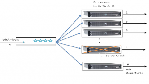
Figure 1. Multi server system with breakdowns, repairs and rebooting delays
The work carried out here clearly depict batch arrivals and batch servicing queuing system where the service channel deals with providing multiservice. It has been assumed that these servers are subject to breakdowns independently or as a cluster. The servers have been repaired either independently or globally based on the nature of the constraints. The arrivals of the customers may follow independent rate or batch-wise while the arrivals follow the compound Poisson process with a batch size of random variable. The system considered the packet arrivals according to a Poisson process with rate σi, where i represent the size of the packets. The service times are drawn with a Poisson distribution µi where i represent the size of the packets. The servers are prone to breakdown when the servicing packets either move to other service stations if it is available or shifted to queue. The servers sit ideally if the queue is empty and one of the servers selected randomly if packets arrive. Figure 1 presents the schematic representation of the system, where customers arrive from one end and these are serviced by parallel pressers.
The QBD process with M jumps is a Markov process that represents a two-dimensional finite lattice strip. The multi-step jumps leads to a Markov process $\mathrm{X}=\{[\mathrm{I}(\mathrm{t}), \mathrm{J}(\mathrm{t})] ; \mathrm{t} \geq 0\}$, on the state space {0, 1, …., N} * {0, 1,…..,}, where the variable J(t) can jump by arbitrary level j+y, and jump down to the level j-z, but the jump levels of the system must be bounded in either upward or downward direction. The finite level of transaction matrices takes the following form:
Aj, Bj,s (s=1, 2,…., y) and Cj,s (s=1, 2,…., z) are the transition rate matrices associated with above mentioned system respectively.
Further the lateral transition matrix for $0 \leq j \leq k$; can be simplified as:
$A_{j}(i, k)=\left\{\begin{array}{c}A_{j}(i, k) \text { for } \cdot 0 \leq i, k \leq \text {Nwheni} \neq j \\ A_{j}(i, k)-\text {Zwheni}=k\end{array}\right.$ (1)
where,
$z=\sum_{l=0}^{N} A_{j}(i, l)-\sum_{s=1}^{y} \sum_{l=0}^{N} B_{j, s}(i, l)-\sum_{s=1}^{z} \sum_{l=0}^{N} C_{j, s}(i, l)$
It is assumed that there is a threshold M, M³y such that
$A_{j}=A, j \geq M ; B_{j, s}=B_{s,} j \geq M-z_{1} ; C_{j, s}=C_{s,} j \geq M$ (2)
This applied for all possible values of s.
The arrival and service processes are modeled for a continuous-time, irreducible Markov phase process with N states that is irreducible. Let Q be the generator matrix of this Markov process. The off diagonal element Q(i, k)=qi,k (i≠k) represents the instantaneous transition rate from phase i to phase k, and the iih diagonal element Q(i,i) = -qi,= $\sum\nolimits_{m=1}^{N}{{{q}_{i,m}}}$ with qi,i=0 with i=1,2,….N, and it is given by:
$Q=\left[ \begin{matrix} -{{q}_{1}} & {{q}_{1,2}} & \cdots & {{q}_{1,N}} \\ {{q}_{2,1}} & -{{q}_{2}} & \cdots & {{q}_{2,N}} \\ \vdots & \ddots & \ddots & \vdots \\ {{q}_{N,1}} & {{q}_{N,2}} & \cdots & -{{q}_{N}} \\\end{matrix} \right]$ (3)
Let r=[r1, r2,…., rN] be the vector of equilibrium probabilities of the modulating phases. Then, r is uniquely determined by the equations:
rQ = 0; re = 1 (4)
e represents the column vector with N elements, whose values are one. Several generalizations and extensions of the model described above are possible. The transition matrices can help in generating equations. Equations (3) and (4) can be expressed as Aj , Bj,s , Cj,s.
The steady-state probabilities have to be determined. The objective of the presented analysis is to determine the steady-state probability Pi,j for the state (i, j) in terms of the known parameters as:
${{P}_{i,j}}=\underset{t\to \infty }{\mathop{Lt}}\,P\{I(t)=i,J(t)=j\};\begin{matrix} {} & {} \\\end{matrix}i=0,1,2,.....$ (5)
The important task is to determine these probabilities in terms of known parameters of the system.
The row vector vj can be defined as:
${{v}_{j}}={{({{p}_{0,j}},{{p}_{1,j}},\ldots {{p}_{N,j}})}_{{}}}{}^{_{{}}}j=0,1,2,\ldots $ (6)
If the process is irreducible and ergodic, then the balance equations corresponding to the state probabilities have a unique normalized solution.
The total sum of all probabilities is always one.
$\sum\nolimits_{j=0}^{\infty }{{{V}_{j}}e=1.0}$ (7)
The balance equations for j = 0, 1, . . . , M − 1 are:
$v_{j} A_{j}+\sum_{s=1}^{y} v_{j-s} B_{j-s, s}+\sum_{s=1}^{\bar{z}} v_{j+s} C_{j+s, s}=0$ (8)
It is assumed that Vj-s=0 if j<s. The corresponding j-independent set for j≥M is represented in mathematical form as equation (8)
$v_{j} A_{j}+\sum_{s=1}^{y} v_{j-s} B_{j-s, s}+\sum_{s=1}^{\bar{z}} v_{j+s} C_{j+s, s}=0$ (9)
Equation (7) can be rewritten in vector difference form of order z=y+zs, with constant coefficients:
$\sum\nolimits_{k=0}^{z}{{{V}_{j+k}}{{Q}_{k}}=0};_{{}}^{{}}j\ge M-{{z}_{1}}$ (10)
Here
$Q_{k}=B_{y-k}$ for $k \leq z-1 ; Q_{y}=A$ and $Q_{k}=C_{k-y}$ fory $\leq k \leq z$
The corresponding matrix polynomial is
$Q(\lambda )=\sum\nolimits_{k=0}^{z}{{{Q}_{k}}{{\lambda }^{k}}}$ (11)
For the computational process, eigen value-eigenvector problem of degree t of a polynomial can be transformed into a linear one. If Qz is non-singular, equation (9) leads to the form.
$\varphi [\sum\nolimits_{k=0}^{z-1}{{{T}_{k}}{{\lambda }^{k}}}+I{{\lambda }^{z}}]=0$ (12)
where, $T_{k}=Q_{k} Q_{z}^{-1}$ Now introducing the vectors $\phi_{k}=\lambda^{k} \varphi$, k=1, 2,...., y–1, the equivalent linear form can be obtained.
$[{{\phi }^{{}}}{{\varphi }_{1}}{{....}_{{}}}{{\varphi }_{z-1}}]\left[ \begin{matrix} 0 & {} & {} & -{{T}_{0}} \\ I & {} & {} & -{{T}_{1}} \\ {} & \ddots & \ddots & {} \\ {} & {} & I & -{{T}_{z-1}} \\\end{matrix} \right]=\lambda [{{\phi }^{{}}}{{\varphi }_{1}}{{....}_{{}}}{{\varphi }_{z-1}}]$ (13)
With the help of eigenvalues and left eigenvectors, the normalized solution of equation (9) can be expressed in the form.
${{V}_{j}}=\sum\nolimits_{k=0}^{c-1}{{{a}_{k}}{{\varphi }_{k}}{{\lambda }^{j-M+{{z}_{1}}}}};_{{}}^{{}}j=M-{{z}_{1}},M-{{z}_{1}},+1,M-{{z}_{1}}+2,....$ (14)
λk represents all the eigenvalues of Q(λ) strictly inside the unit disk φk are their corresponding independent eigenvectors, and ak are the arbitrary constants. The latter constants are determined with the aid of the state-dependent balance equations, that is for $j \leq M-1$, and the normalization equation.
2.1 Stability of the system
It is important to ensure the stability of the system. The system is stable if it follows the given condition and has the feasible solution. Let us consider the row vector, V=(q0, q1,….,qN) where $q_{i} \geq 0$; i=0, 1,…., N. The necessary condition for the stability of the system with the balance equations (8) and (9) can be expressed in the following form:
$V[A-{{D}^{A}}+\sum\nolimits_{s=1}^{{{z}_{1}}}{({{B}_{s}}-D_{s}^{B})}+\sum\nolimits_{s=1}^{{{z}_{2}}}{({{C}_{s}}-D_{s}^{C})};\begin{matrix} {} & {} \\\end{matrix}Ve=1;$ (15)
where, DA, DsB and DsC are the diagonal matrices whose ith diagonal element is the sum of its corresponding row of the respective matrices.
The inequality condition for the stable of the system is expressed as:
$V[\sum\nolimits_{s=1}^{{{z}_{1}}}{s{{B}_{s}}]e}<V[\sum\nolimits_{s=1}^{{{z}_{2}}}{s{{C}_{s}}]e}$ (16)
3.1 Results with batch services
In this section, the results obtained have been picturized in graphical form. The performance measures have been considered where customers arrive either independent or batches. The size of the batch may be 2, 3, 4 or a higher number. Similarly, the services of the customers are done either independently or with batches. In this paper, an efficient algorithm is developed to generate the simulation results in spectral expansion. If the transient state of the system is unstable, the performance measures are complicated to analyze. In such cases, the performance measures for steady-state aspects have been taken into consideration. During the process of computation of performance measures in this work, the parameters, unless otherwise not mentioned are taken as ξ=0.1, η=0.1, ξ0=0.05, ηn=0.1, μ=1.5 and the number of servers is fixed have been fixed as 10.
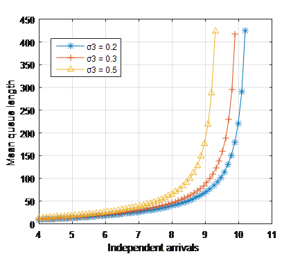
Figure 2 presents the result for mean queue length with independent arrivals of the customers by taking the arrivals of batch size 3 is 0.25. Here, batch size 2 customer's arrival rate is fixed with 0.2, 0.5 and 0.8. Results are presented in graphical form. It is observed that the length of the queue is proportionately increased with customer arrivals. Figure 3 is similar to Figure 2 and the results are presented for mean queue length with the mean arrival rate of batch size 3. In this graph, independent arrivals of the customers are placed with 6.0 and results are presented for batch size 2 by taking 0.2, 0.3 and 0.5. It can be observed that queue length increases rapidly as the arrivals of the customers come up to 3 folds.
Figure 2. Waiting time versus arrivals of the customers with 0.1 batch size 3 customers
Figure 3. Waiting time versus batch arrivals of the customers with 6 independent arrivals
Figure 4. Queue size versus independent service of the customers
Figures 4 and 5 present the results for waiting time with mean service rates. With these results, it is observed that the waiting time inversely decreases concerning service rates. Figure 4 presents the results for the independent service rate by setting independent arrival rate σ=1, 3, 5. Here, batch size 2 customer arrivals fixed with 0.5 and batch size 3 with 0.2. Whereas in Figure 5, the independent service rate is fixed at 0.25 and results are presented for batch size 2 service rate of the customers. Figures 6 and 7 present the results for mean queue length for waiting time with independent arrivals and mean arrivals of batch size 2 respectively. In Figure 6 the batch size 2 is fixed as 0.5 and single service rate as 1.5. In Figure 7, the service rate is taken as 2 with independent service rate 1.5 and batch 2 service rates with 0.3.
Figure 5. Waiting time versus multiple service rate arrivals
Figure 6. Waiting time versus multiple service rate arrivals
Figure 7. Waiting time versus independent arrivals with different levels of batch size arrivals of 2
3.1 Results with independent service
The results are presented with independent arrival and batch size 2, the service of the customer performed independently and batch service restricted. As mentioned earlier, the various parameters have been considered and results are presented in graphical form. Figures 8 and 9 present the results for waiting time with different arrival rates. Figure 8 presents results for independent arrivals with batch sizes 0.2, 0.3, and 0.5, whereas, in Figure 9, customers arrive as batches with size 2.
Figure 8. Waiting time versus arrivals of the customers with 0.1 batch size 3 customers
Figure 9. Waiting time versus batch arrivals of the customers with 6 independent arrivals
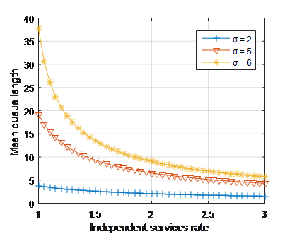
Figure 10. Queue size versus independent service of the customers
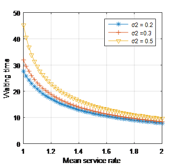
In Figure 9, independent arrivals of the customers are fixed with σ=2, 5, 6 and batch size 2 with 0.25. Figures 10 and 11 present the result for mean service rates with different arrivals. In Figure 10, the batch size 2 is fixed with 0.25 by considering independent arrivals 2, 5, and 6 and in Figure 11, batch size 2 is fixed with 0.2, 0.3, and 0.5 along with independent arrivals 6. Figure 12 presents the result for queue length with customer arrival with variable service rates proportionate to independent arrivals with a rate of 0.75. With this graph, it is observed that queue length increases linearly to the arrivals.
Figure 11. Waiting time versus multiple service rate arrivals
Figure 12. Waiting time versus multiple service rate arrivals
An efficient model has been designed that takes into consideration a large number of parameters and assesses the manner in which waiting rate changes depending on a number of servers. With most of the real-world applications being dynamic, the designed model takes into consideration the arrival rate and predicts the average waiting time of. This, in turn, could help in predicting the need for increase or decrease in servers in a system thereby minimizing both the waiting as well as the idle times. The cases have been predicted both for independent arrivals and arrivals in batches. Another novelty in this technique lies in the fact that variations have been predicted with changes in batch size. Results clearly indicate the variations in mean service time with respect to batches. Taking this view into perspective, a dynamic model can be introduced for a given application that automatically increases the number of servers during peak periods and reduces the same during lean periods.
The authors wish to express their gratitude to the anonymous referees and the editor for their valuable guidelines and suggestions for refinement of the paper.
[1] Van Do, T., Chakka, R., Sztrik, J. (2013). Spectral expansion solution methodology for QBD-M processes and applications in future internet engineering. In Advanced Computational Methods for Knowledge Engineering. Springer, Heidelberg, pp. 131-142. https://doi.org/10.1007/978-3-319-00293-4_11
[2] Wang, Y.C., Chou, J.H., Wang, S.Y. (2011). Loss pattern of DBMAP/DMSP/1/K queue and its application in wireless local communications. Applied Mathematical Modelling, 35(4): 1782-1797. https://doi.org/10.1016/j.apm.2010.10.009
[3] Mamatha, E., Sasritha, S., Reddy, C.S. (2017). Expert system and heuristics algorithm for cloud resource scheduling. Romanian Statistical Review, 65(1): 3-18.
[4] Ezhilchelvan, P.,Mitrani, I. (2019). Multi-class resource sharing with batch arrivals. Probability in the Engineering and Informational Sciences, 33(3): 348-366. https://doi.org/10.1017/S0269964818000323
[5] Chakravarthy, S.R. (2001). The batch Markovian arrival process: A review and future work. Advances in Probability Theory and Stochastic Processes, 1: 21-49.
[6] Chakravarthy, S.R., Maity, A., Gupta, U.C. (2017). An ‘(s, S)’inventory in a queueing system with batch service facility. Annals of Operations Research, 258(2): 263-283. https://doi.org/10.1007/s10479-015-2041-z
[7] Patil, R., Gade, A., Rewatkar, A. (2019). Comprehensive study on task scheduling strategies in multicloud environment. Journal Europeen des Systemes Automatises, 52(1): 43-47. https://doi.org/10.18280/jesa.520106
[8] Van Do, T. (2010). M/M/1 retrial queue with working vacations. Acta Informatica, 47(1): 67-75. https://doi.org/10.1007/s00236-009-0110-y
[9] Banerjee, A., Gupta, U.C., Chakravarthy, S.R. (2015). Analysis of a finite-buffer bulk-service queue under Markovian arrival process with batch-size-dependent service. Computers & Operations Research, 60: 138-149. https://doi.org/10.1016/j.cor.2015.02.012
[10] Mamatha, E., Saritha, S., Reddy, C.S. (2019). Performance measures of online warehouse service system with replenishment policy. Journal Européen des Systèmes Automatisés, 52(6): 631-638. https://doi.org/10.18280/jesa.520611
[11] Sama, H.R., Vemuri, V.K., Talagadadeevi, S.R., Bhavirisetti, S.K. (2019). Analysis of an N-policy MX/M/1 two-phase queueing system with state-dependent arrival rates and unreliable server. Ingénierie des Systèmes d’Information, Vol. 24, No. 3, pp. 233-240. https://doi.org/10.18280/isi.240302
[12] Choudhury, G., Madan, K.C. (2004). A two phase batch arrival queueing system with a vacation time under Bernoulli schedule. Applied Mathematics and Computation, 149(2): 337-349. https://doi.org/10.1016/S0096-3003(03)00138-3
[13] Sikdar, K., Samanta, S.K. (2016). Analysis of a finite buffer variable batch service queue with batch Markovian arrival process and server’s vacation. Opsearch, 53(3): 553-583. https://doi.org/10.1007/s12597-015-0244-3
[14] Mamatha, E., Saritha, S., Reddy, C.S. (2016). Stochastic scheduling algorithm for distributed cloud networks using heuristic approach. International Journal of Advanced Networking and Applications, 8(1): 3009.
[15] Chakka, R., Harrison, P.G. (2001). A Markov modulated multi-server queue with negative customers-the MM CPP/GE/c/L G-queue. Acta Informatica, 37(11-12): 881-919. https://doi.org/10.1007/PL00013307
[16] Lee, H.W., Moon, J.M., Kim, B.K., Park, J.G., Lee, S.W. (2005). A simple eigenvalue method for low-order D-BMAP/G/1 queues. Applied Mathematical Modelling, 29(3), 277-288. https://doi.org/10.1016/j.apm.2004.07.004
[17] Goswami, V., Mund, G.B. (2009). Multiserver bulk service discrete-time queue with finite buffer and renewal input. Computers & Mathematics with Applications, 57(8): 1377-1388. https://doi.org/10.1016/j.camwa.2009.01.033
[18] Niu, Z., Shu, T., Takahashi, Y. (2003). A vacation queue with setup and close-down times and batch Markovian arrival processes. Performance Evaluation, 54(3): 225-248. https://doi.org/10.1016/S0166-5316(03)00058-0
[19] Choudhury, G., Paul, M. (2006). A batch arrival queue with a second optional service channel under N-policy. Stochastic Analysis and Applications, 24(1): 1-21. https://doi.org/10.1080/07362990500397277
[20] Dimitriou, I. (2013). A preemptive resume priority retrial queue with state dependent arrivals, unreliable server and negative customers. Top, 21(3): 542-571. https://doi.org/10.1007/s11750-011-0198-4
[21] Mamatha, E., Reddy, C.S., Prasad, R. (2012). Mathematical modeling of markovian queuing network with repairs, breakdown and fixed buffer. i-Manager's Journal on Software Engineering, 6(3), 21.
[22] Hanschke, T. (2006). Approximations for the mean queue length of the GIX/G (b, b)/c queue. Operations Research Letters, 34(2): 205-213. https://doi.org/10.1016/j.orl.2005.01.011